Electromagnetic wave response and intelligent recognition of defects at reconstructed and expanded roadbed junctions

During the reconstruction and expansion of expressways, defects at the roadbed junction can compromise driving safety and significantly reduce the service life of the road. Based on engineering cases, a generalized model of the defective reconstructed and expanded roadbed junction was developed, and the propagation simulation of electromagnetic waves in the defective roadbed junction was performed using the finite-difference time-domain (FDTD) method. The simulation results demonstrated that the electromagnetic waves formed two sets of parallel convex hyperbolas at the circular cavity defects. The presence of non-compactness defects caused the overall reflected wave signal to exhibit an imaging characteristic with a clear upper section and a blurred lower section. In addition, electromagnetic waves manifested as multiple nearly parallel convex hyperbolas near the vertical cracks. On this basis, by integrating numerical simulation results with field-measured data, a comprehensive dataset encompassing various types of defects was established. Following the optimization of the YOLO algorithm training model, the identification accuracy rates for void, non-compactness, and crack defects reached 97%, 99%, and 99%, respectively. The new method proposed in this study has universal reference value and application potential for road defect detection under different geological conditions and construction standards.

1 Introduction

By the end of 2023, the total mileage of highways in China had exceeded 5.4368 million kilometers, with fourth-grade highways comprising 73.8% of the network and playing a crucial role in delivering transportation services. With the deepening of the strategy to build a strong transportation nation, reconstructing and expanding existing highways have become critical measures for optimizing the road network structure and enhancing service efficiency. However, structural defects, such as longitudinal cracks that frequently occur at the junction between the new and old roadbeds, not only significantly shorten the service life of the road but also increase the annual maintenance cost by 15%–30%, thereby posing a serious threat to driving safety (Zhang et al., 2024). This current situation places higher demands on road defect detection technology.

In the field of non-destructive detection of concealed road defects, ground-penetrating radar (GPR) technology has gained widespread adoption owing to its exceptional efficiency and high-resolution capabilities (Yu et al., 2023; Liu et al., 2025). However, due to the multi-phase characteristics of roadbed materials and the intricate morphology of defects, traditional interpretation methods encounter bottlenecks, including insufficient feature extraction and a high misjudgment rate (Wang et al., 2024; Tešić et al., 2021; Morris et al., 2021). In recent years, GPR technology has made breakthrough progress in multiple dimensions: In terms of hardware innovation, Guo et al. (2023) revealed the influence of antenna quality on the imaging effect by comparing the performance of different antennas in railroad ballast layer detection. Tesic et al. (2022) elucidated the mechanism of sodium chloride solution distribution on GPR signaling amplitude through accelerated corrosion experiments. Zhang et al. (2022) developed a three-dimensional reconstruction model for a landfill using the travel time of electromagnetic waves, thereby extending the applicability of GPR in achieving high spatial resolution. At the software algorithm level, (Xu et al., 2024) adopted the UNet network to achieve the identification accuracy of 88% of the rock layer. Zhou et al. (2023) used the VRADI algorithm combined with DBSCAN clustering, which improved the accuracy of void recognition to 92.2%. Tang et al. (2022) improved the MPA index of crack segmentation by 12.6% through the Crack UNet model optimized by the attention mechanism. Puntu et al. (2021) developed a tunnel-lining boundary detection system and verified the engineering applicability of the Fresnel reflection coefficient. Abdelsamei et al. (2024) established an amplitude feature evaluation system to achieve millimeter-level detection accuracy of pavement thickness. It is noteworthy that 3D GPR technology (Lv et al., 2023; Amaral et al., 2023) has demonstrated unique advantages in complex engineering scenarios through multi-channel data fusion and physical experiment verification.

With the deep integration of artificial intelligence technology, the GPR intelligent diagnosis system is driving the innovation of the detection paradigm. In terms of feature extraction, the frequency band dielectric spectrum analysis developed by Zhang et al. (2018) can identify early defects with 0.5% water content. Bu et al. (2025) established a time-frequency fusion model and improved the defect identification accuracy to 91.6%. At the level of algorithm optimization, Guo et al. (2022) proposed a CEEMD-aligned entropy noise reduction method to effectively suppress signal interference. Sonoda and Nakamichi (2024) significantly improved the robustness of deep learning models through Cutout data enhancement technology. The LSTM wavelet network designed by Geng et al. (2022) achieved clutter suppression without prior information. The high-level FDTD (2, 4) code developed by Chi et al. (2024) effectively improved the recognition ability of shallowly buried targets. Li et al. (2024) proposed an adaptive curriculum learning framework, reducing the false detection rate in urban scenes to 2.1%. The MHUnet-YOLOv8 model constructed by Kan et al. (2024) achieved a breakthrough in void detection accuracy. Although existing research has established a relatively complete roadbed defect identification system, there is still a significant gap in the detection technology for the special working conditions of the reconstructed and expanded roadbed junction.

In summary, numerous scholars have utilized deep learning to extract and learn features from classified GPA imaging data, establishing automatic identification technologies for roadbed defects. However, there are limited relevant findings regarding defects at the junction of reconstructed and expanded roadbeds. This study develops a generalized model of roadbed junction defects based on extensive field research and establishes a radar imaging data sample library for roadbed junction defects by integrating numerical simulations with field test data. On this basis, an intelligent identification model for the reconstructed and expanded roadbed junction is established by employing an enhanced deep learning algorithm, thereby providing a reliable reference for the maintenance of operational highways, as well as reconstruction and expansion projects.

2 Forward modeling based on finite-difference time-domain methods

2.1 Basic principles of radar wave testing

GPR transmits high-frequency broadband electromagnetic waves into the ground through a transmitting antenna and receives the electromagnetic waves through a receiving antenna. Reflection occurs when an electromagnetic wave impinges upon the junction between two materials with differing dielectric properties. A greater difference in the dielectric properties of the two materials indicates a stronger reflected signal of the electromagnetic wave. Numerous reflected waves constitute the radar profile image, as shown in Figure 1. According to the waveform, amplitude, and echo time of the reflected wave, the geometric shape, material characteristics, and position of the detection target can be interpreted.

Figure 1

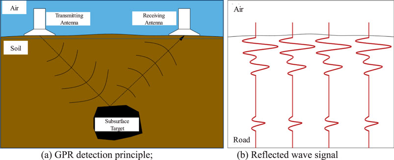
Figure 1. Working principle of GPR. (a) GPR detection principle; (b) Reflected wave signal.

2.2 Finite-difference time-domain method

Finite-difference time-domain (FDTD) is a numerical method for solving electromagnetic field problems with high accuracy and stability. The FDTD method is based on Maxwell’s equations and the constitutive relationship of materials. It can effectively simulate the propagation characteristics of electromagnetic waves in complex media and provide theoretical support for GPR signal analysis. Here the Perfectly Matched Layer boundary conditions are used.

This method demonstrates high accuracy and reliability when applied to the calculation of electromagnetic field problems. Additionally, it facilitates a deeper understanding and more precise prediction of the propagation characteristics of electromagnetic waves in complex environments.

Combining the Maxwell equations and the constitutive relation of the electromagnetic field, the Maxwell equations of TM waves in a two-dimensional rectangular coordinate system are obtained, as shown in Equations 1–3:

$\frac{\mathrm{\partial }{E}_z}{\mathrm{\partial }y}=-\mu \frac{\mathrm{\partial }{H}_x}{\mathrm{\partial }t}-{\sigma }_m{H}_x(1)$

$\frac{\mathrm{\partial }{E}_z}{\mathrm{\partial }x}=\mu \frac{\mathrm{\partial }{H}_y}{\mathrm{\partial }t}+{\sigma }_m{H}_y(2)$

$\frac{\mathrm{\partial }{H}_y}{\mathrm{\partial }x}-\frac{\mathrm{\partial }{H}_x}{\mathrm{\partial }y}=\epsilon \frac{\mathrm{\partial }{E}_z}{\mathrm{\partial }t}+\sigma E_z(3)$

where E _Z is the electric field strength in the z direction; H_x and H_y are the magnetic field strengths in the x and y directions, respectively; σm is the magnetic resistivity for calculating magnetic loss; σ is the electrical conductivity of the medium; ε is the relative dielectric constant; μ represents the magnetic permeability. The model established in this paper does not include magnetic materials, that is, σm = 0, μ = 1.

The electric field and magnetic field have the characteristic of alternating sampling in the time series, and their sampling intervals differ from each other by half a time step. Therefore, the FDTD equation of the two-dimensional TM wave is Zhang et al. (2011) as shown in Equations 4–6:

$H_x^{n+\frac{1}{2}}\left(\mathrm{i},\mathrm{j}+\frac{1}{2}\right)=H_x^{n-\frac{1}{2}}\left(\mathrm{i},\mathrm{j}+\frac{1}{2}\right)-\frac{\Delta t}{\mu ·\Delta y}\left[E_z^n\left(\mathrm{i},\mathrm{j}+1\right)-E_x^n\left(\mathrm{i},\mathrm{j}\right)\right](4)$

$H_y^{n+\frac{1}{2}}\left(\mathrm{i}+\frac{1}{2},\mathrm{j}\right)=H_y^{n-\frac{1}{2}}\left(\mathrm{i}+\frac{1}{2},\mathrm{j}\right)+\frac{\Delta t}{\mu ·\Delta \mathrm{x}}\left[E_z^n\left(\mathrm{i}+1,\mathrm{j}\right)-E_z^n\left(\mathrm{i},\mathrm{j}\right)\right](5)$

$\begin{array}{l}{E}_z^{n+1}\left(i,j\right)=\frac{\epsilon -\frac{\sigma \Delta t}{2}}{{\epsilon }^{+\frac{\sigma \Delta t}{2}}}{E}_z^n\left(i,j\right)+\frac{\Delta t}{\left(\epsilon +\frac{\sigma \Delta t}{2}\right)\Delta x}\left[H_y^{n+\frac{1}{2}}\left(i+\frac{1}{2},j\right)-H_y^{n+\frac{1}{2}}\left(i-\frac{1}{2},j\right)\right]\\ -\frac{\Delta t}{\left(\epsilon +\frac{\sigma \Delta t}{2}\right)\Delta y}\left[H_x^{n+\frac{1}{2}}\left(i,j+\frac{1}{2}\right)-H_x^n\left(i,j-\frac{1}{2}\right)\right]\end{array}(6)$

where E_z is the electric field intensity; H_x and H_y are the magnetic field intensities; Δt is the time step; n is the discrete time; Δx and Δy are the spatial steps of the Yee cell in the x and y directions, respectively; (i, j) is the grid space coordinate.

3 Simulation of electromagnetic wave propagation in reconstructed and expanded roadbeds

3.1 Generalized model of the defect at the reconstructed and expanded roadbed junction

The development of a generalized roadbed model incorporating various defect types serves as the foundation for analyzing the propagation characteristics of electromagnetic waves at the junction of defective reconstructed and expanded roadbeds. Affected by both natural and man-made factors, including geological characteristics, hydrological meteorology, vehicle loads, and construction technology, three typical defects-voids, non-compactness, and cracks-have emerged during the reconstruction and expansion of roadbeds. This study focuses on a highway expansion and reconstruction project in Yichun City, Jiangxi Province. The step method was employed to widen the roadbed on both sides. Specifically, the step height and width were both set to 1 m. Half of the roadbed on each side after widening was selected for simulation, with the model having a side length of 8 m and a depth of 7 m.

Based on the reconstruction and expansion of the roadbed structure, the generalized model is simplified to include air, the existing roadbed, the newly constructed roadbed, and defects. Among them, the generalized model of the circular void defect is shown in Figure 2a, where the radius of the void is 0.3 m, and the void is filled with air. The horizontal position of the circular void is randomly determined within the range of 0.80 m–7.15 m, with a precision of two decimal places. The buried depth is also randomly assigned within the range of 0.60 m–6.50 m, maintaining the same level of precision. Both parameters, the horizontal position and the buried depth, jointly define the location of the circular void. A total of 82 working conditions are established based on these parameters. The generalized model representing the non-compactness defect is illustrated in Figure 2b. A square region is defined at the junction between the new and old roadbeds. A random seeding approach is employed within this square region, where half of the area is designated as void space to simulate a compaction degree of 50%. The non-compactness region has a total area of 0.25 m × 0.25 m. The horizontal position is randomly selected within the range of 0.8 m–6.9 m, with values specified in two decimal places. Similarly, the burial depth is randomly determined within the range of 0.5 m–6.0 m, also expressed in two decimal places. The location of the non-compactness region is jointly determined by both the horizontal position and the burial depth. A total of 82 working conditions are established for analysis. The generalized model of the crack defect is presented in Figure 2c. In this model, the crack is approximated as an assembly of small rectangular cavities with contacting boundaries, and various crack configurations are simulated through a staggered arrangement of these cavities. The length of the crack is 0.65 m. The horizontal position is randomly selected within the range of 1.60 m–7.00 m, with values specified to two decimal places. The burial depth is randomly set between 0.50 m and 6.40 m, also with values specified to two decimal places. The location of the crack is determined jointly by its horizontal position and burial depth, and a total of 82 working conditions are established.

Figure 2

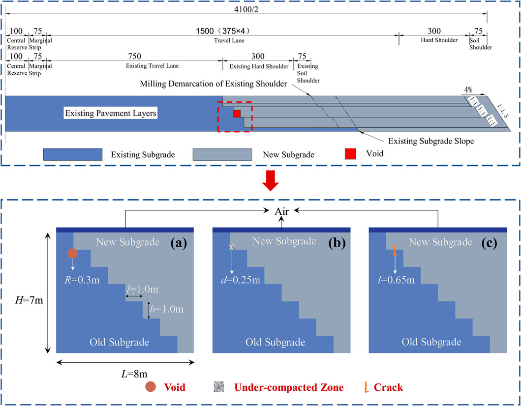
Figure 2. Generalized model of typical defects at the junction of the reconstructed and expanded roadbed: (a) Void, (b) Under-compacted zone, (c) Crack.

3.2 Assumptions

The reconstructed and expanded roadbed is mainly filled with coarse-grained soil. The filling soil utilized in actual engineering projects is not comprised of a single, homogeneous soil type but rather constitutes a mixture of several soils with varying properties and proportions. Moreover, the physical characteristics of the soil are subject to variation due to the impact of construction techniques and the specific conditions of the roadbed paving environment. The relative dielectric constant of soil is closely related to factors such as soil stone content, compaction, porosity, water content, humidity, temperature, ion type, and clay mineral content. These factors are coupled with each other and are difficult to decouple (Park et al., 2017; Wagner et al., 2011; Ling et al., 2016). Due to the challenges in accurately simulating the real relative permittivity of coarse-grained soil in the expanded and renovated roadbed under the coupling effect of the aforementioned factors using existing methods and taking into account practical constraints such as computational power, the following assumptions are made when setting model parameters for forward simulation:

1. Assuming that the soil of the reconstructed and expanded roadbed is a homogeneous medium composed of the same type of soil;

2. Assuming that the relative dielectric constant of the soil remains constant, the arithmetic mean of the measured field data is selected for analysis;

3. Assuming that the resistivity of the soil is constant, the arithmetic mean of the field-measured data is selected;

4. The voids in the reconstructed and expanded roadbed are simplified as circular shapes filled with air, while cracks and non-compactness regions are modeled as defects resulting from the interconnected combination of several minute rectangular voids, also filled with air;

5. Assuming that both the signal transmitting and receiving points are located on the contact surface between the soil and air of the reconstructed and expanded roadbed.

3.3 Material parameters

The reconstructed and expanded roadbed is simulated with loose soil, air, and water. The values of various material properties and their corresponding electrical characteristic parameters are presented in Table 1. Among them, the material simulating the roadbed is referred to as the primary medium, while the material used for defect simulation is termed the filling medium.

Table 1

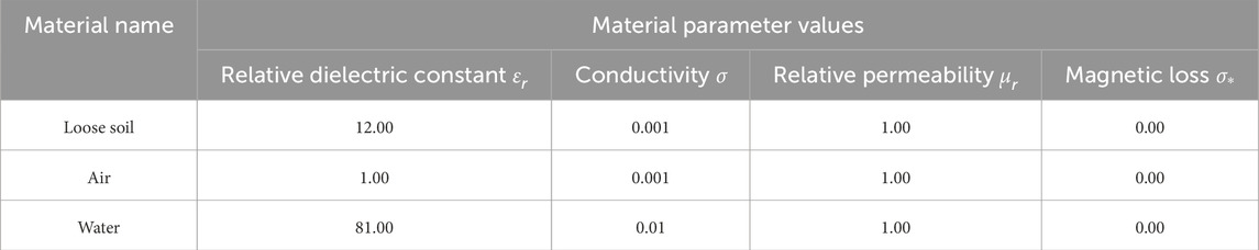
Table 1. Material parameters.

3.4 Propagation characteristics

The propagation of electromagnetic waves at the junction of the reconstructed and expanded red sandstone roadbed, which contains circular void defects, is illustrated in Figure 3a. By observing the hyperbolic features in the defect image, it can be found that under the influence of a single circular void defect, the electromagnetic wave exhibits two sets of parallel convex hyperbolas at the defect location. The top set of hyperbolas is clearly more distinct than the bottom set. The propagation of electromagnetic waves in the junction of the reconstructed and expanded red sandstone roadbed containing non-compactness regions is shown in Figure 3b. By analyzing the hyperbolic characteristics in the defect image, it is evident that the presence of non-compactness defects causes the overall reflected wave signal to exhibit an imaging feature with a sharp upper section and a diffuse lower section. Compared with the imaging characteristics of void defects, the imaging of non-compactness defects is more complicated. The propagation of electromagnetic waves in the junction of the reconstructed and expanded red sandstone roadbed with cracks is shown in Figure 3c. By analyzing the hyperbolic features in the defect image, it is evident that under the influence of a single vertical crack defect, the image exhibits multiple approximately parallel convex hyperbolas near the defect location. Among all the hyperbolas, the top group exhibits distinct characteristics, whereas the reflected signals of the other hyperbolas below this group at the defect locations are extremely vague and nearly indistinguishable.

Figure 3

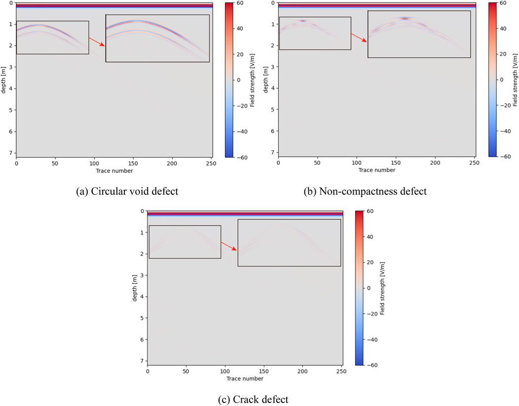
Figure 3. Simulation results of electromagnetic wave propagation in reconstructed red sandstone roadbeds containing different defect types. (a) Circular void defect (b) Non-compactness defect. (c) Crack defect.

Taking non-compactness defects as an example, the influence of different horizontal positions and burial depths of defects on radar wave propagation is explored. The electromagnetic wave propagation for non-compactness defects at varying horizontal positions and the same depth is illustrated in Figure 4a. The red vertical line in the model layout diagram (upper right corner) indicates the horizontal position of the center of the non-compactness defect and serves as a positional reference for the defect imaging information presented in the upper left corner. Analysis reveals that at the same depth, the hyperbolic patterns in the electromagnetic wave propagation maps of non-compactness defects at different horizontal positions are essentially identical, with variations observed only in their horizontal locations. This indicates that the horizontal position of a circular void defect can be deduced from the location of the hyperbola in the electromagnetic wave propagation image. The electromagnetic wave propagation characteristics of a circular void defect at various horizontal positions but at the same depth are illustrated in Figure 4b. Analysis reveals that when the burial depth of the circular void is 0.5 m, the reflected wave signal is distinct, and there is an evident difference in signal strength among multiple groups of hyperbolas, with a relatively small curve opening. As the burial depth of the circular void progressively increases to 2.65 m, 3.89 m, and 5.8 m, the reflected wave signal gradually weakens, and the curve opening expands with increasing burial depth. When the burial depth reaches 5.8 m, the reflected wave signal becomes blurred and almost unrecognizable.

Figure 4

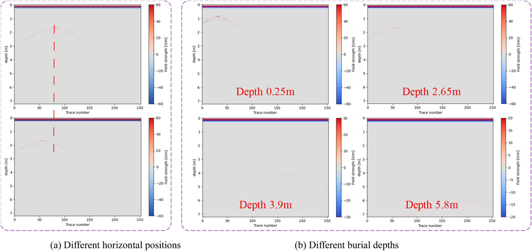
Figure 4. Simulation results of electromagnetic wave propagation in the expanded red sandstone roadbed with void defects. (a) Different horizontal positions (b) Different burial depths.

4 GPR field detection

4.1 Field test scheme

The test was carried out in the reconstruction and expansion project of the G60 Expressway, located in the Yichun section of Jiangxi Province, China, as illustrated in Figure 5. The expressway has been in operation for many years and the roadbed soil has been compacted to the maximum extent. The on-site survey results indicate multiple defects in the roadbed, including slope collapse, ruts, and voids. Additionally, numerous locations exhibit damaged shoulders and uneven settlement of the roadbed. Therefore, the newly constructed roadbed was selected for experimental testing. Through geological survey analysis, early construction monitoring measurement data, road design drawings, and other relevant information, while considering the road width and anticipated detection depth, it is comprehensively determined that the survey lines should be arranged symmetrically with the road centerline as the axis and a spacing of 3 m on both sides. This arrangement ensures adequate coverage and resolution for effective detection. For the junction area of the new and old roadbeds, the spacing of the measuring lines is reduced to 1 m to enhance the detection accuracy. The on-site detection area is shown in Figure 6a. The on-site testing equipment is a GPR produced by Qingdao China Electronics Zhongyi Intelligent Technology Development Co., Ltd. This equipment includes the GER-10 radar host, GER400A ground coupling antenna, and ranging wheel (circumference 450 mm, pulse number 500), as shown in Figure 6b. The antenna frequency is 100 MHz.

Figure 5

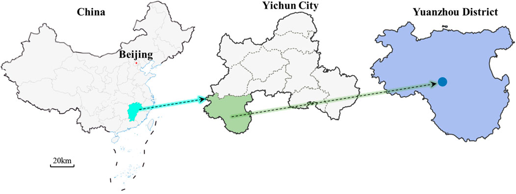
Figure 5. Field testing location map.

Figure 6

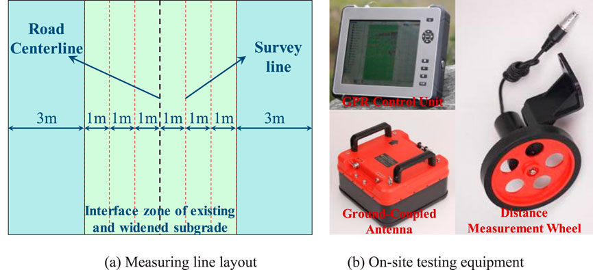
Figure 6. Measuring line layout and test equipment. (a) Measuring line layout (b) On-site testing equipment.

4.2 GPR imaging characteristics of roadbed junction defects

The electromagnetic wave propagation characteristics for various types of defects measured in the field are presented in Figure 7. Multiple sets of smooth, band-shaped hyperbolic reflected signals extending towards the road surface are observed at the location of the circular void defect. These signals exhibit characteristics that are largely consistent with those of the simulated defect. The non-compactness defect develops below the junction between the new and old roadbeds. Compared with the simulated non-compactness defect, the image of the real non-compactness defect contains more hyperbolic groups and exhibits greater complexity. However, there is no prominent reflected signal at the center of the defect. The signal intensity transitions from the center to both sides demonstrate a repetitive pattern characterized by initial attenuation, followed by enhancement, and then subsequent attenuation. The cracks propagate from the bottom to the top of the road surface and manifest as narrow strip signals composed of multiple groups of hyperbolas on the graph. At the intersection of the contact surface between the roadbed and the pavement with the crack, a concave reflected signal is observed. Compared to simulated defect imaging, the radar imaging of real crack defects exhibits a narrower hyperbola opening and a greater number of hyperbola clusters. The signal distributed vertically along the crack has weaker attenuation and better imaging. In summary, in contrast to the simulated defect image, the real roadbed junction defect image contains substantial noise resulting from non-uniform roadbed materials and inconsistent compaction. This is characterized by the presence of several densely distributed hyperbolic patterns. Therefore, in order to accurately identify various types of defects, it is necessary to process the measured GPR images.

Figure 7

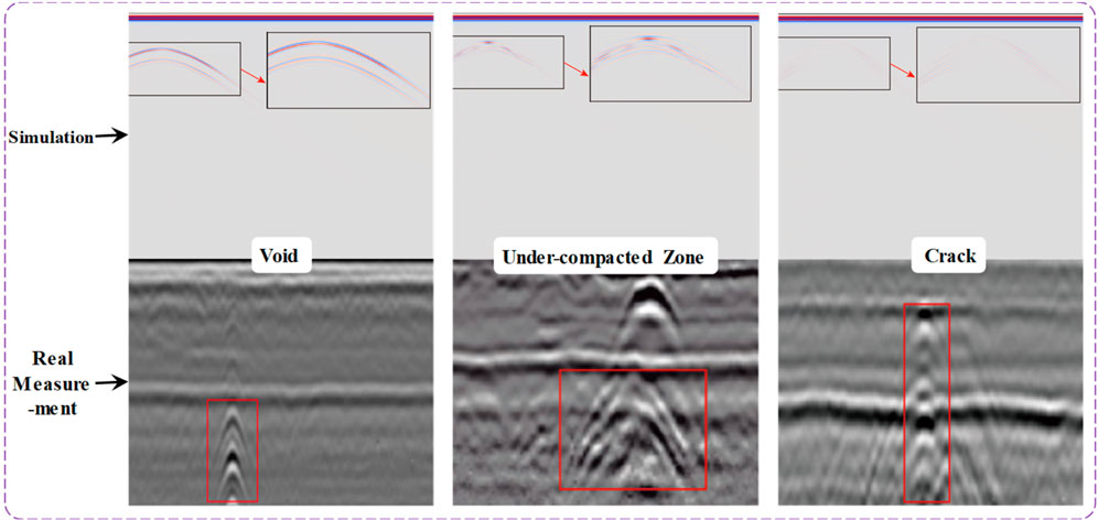
Figure 7. Simulated and measured electromagnetic wave propagation characteristics of different types of defects.

4.3 GPR image processing

After acquiring the GPR image of the red sandstone roadbed with defects, a series of preprocessing steps are necessary to enhance the quality of the model input data and improve the detection performance. The detailed procedures are illustrated in Figure 8. GPR detection aims to comprehensively collect the response signals of the internal structure to radar waves, including effective waves and interference waves. In order to remove the interference signal, filter processing is adopted. Since the time window zero point typically does not align with the ground position, the ground position must be calibrated when calculating the target depth. This involves adjusting the zero point to ensure accurate measurements. Considering the undulations of the terrain, manual adjustment of the zero point may not achieve perfect alignment. Therefore, zero-point correction is employed to automatically detect and adjust for ground position. After correction, the data is balanced by seeking the maximum (positive phase) and minimum (negative phase) values at the specified sampling point. In addition, the electromagnetic wave energy attenuates during medium propagation, necessitating gain adjustment to enhance the imaging features associated with the defect. A common method is to manually adjust the number of gain points and their gain values. Manual gain refers to the process of converting the original data into a gain curve $y\left(t\right)=Ax\left(t\right)\times e^{at}$. The purpose of gain is achieved by changing the adjustment coefficient a.

Figure 8

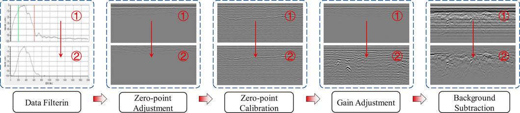
Figure 8. GPR imaging process.

5 Intelligent identification model of roadbed defects based on the YOLO network

5.1 Defect sample dataset

When using convolutional neural networks for object detection in images, the composition of the dataset affects the recognition accuracy. The above-mentioned simulations of the propagation of electromagnetic waves in the reconstructed and expanded roadbed, which contains defects of various types, burial depths, horizontal positions, and geometric sizes, were conducted. A total of 343 ground-penetrating radar forward simulation images of the defects at the junction of the reconstructed and expanded roadbed were generated. To identify the defects occurring at the junction of reconstructed and expanded roadbeds, GPR was employed for on-site detection. This process yielded a total of 900 images depicting voids, cracks, and non-compactness defects at the roadbed junction. Subsequently, a comprehensive roadbed junction defect dataset was constructed, encompassing 1243 images that captured various types of voids, cracks, and non-compactness defects. In order to avoid overfitting and other problems, Mosaic enhancement, random affine transformation, MixUp enhancement, and HSV data enhancement technology were used to expand 5590 GPR images of roadbed junction defects. This model creates and edits annotation boxes on the sample library images through the open source image annotation tool LbelImg, which is used to mark the location and category of the objects. Combined with the original 1,243 images, a dataset comprising 6,833 roadbed junction defect samples was constructed for subsequent model training. The defects included 1,479 rectangular voids, 1,476 circular voids, 1,476 cracks, and 2,402 non-compactness regions. The dataset was split into training and testing sets according to an 8:2 ratio.

5.2 Model architecture

YOLO network is an advanced object detection algorithm based on deep learning. Its core feature is the ability to simultaneously complete the localization and classification of targets on a single image. Compared with traditional object detection algorithms (such as the R-CNN series algorithms), it features fast detection speed, high global perception and positioning accuracy, good adaptability to complex scenes, and a simple model that is easy to deploy, balancing efficiency and practicality, which makes it widely used in scenarios with high real-time requirements. In the YOLOv5 network, target detection is achieved through the output part composed of a loss function and non-maximum suppression (NMS). This algorithm will force the scores of adjacent detection boxes to zero, resulting in failure to detect the object, which is not conducive to the identification of multiple adjacent defects in the same radar image of the reconstructed and expanded roadbed. Therefore, the overall architecture based on the YOLO algorithm was constructed (Wanyan et al., 2024), featuring a backbone network composed of several groups of “CBS-C3” layers and an SPPF layer. Additionally, the head part was designed by integrating C3, upsampling, and multi-scale feature map tensor concatenation operations, thereby forming a “top-down, bottom-up” multi-scale feature fusion algorithm architecture, as illustrated in Figure 9. This architecture can prevent the inability to effectively identify multiple defects in the same location within the reconstructed and expanded roadbed.

Figure 9

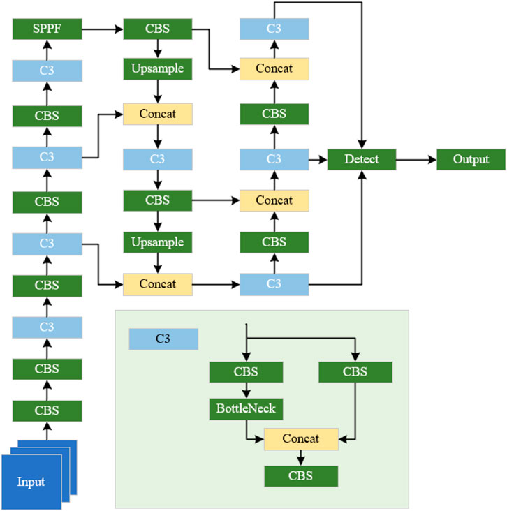
Figure 9. Improved algorithm architecture for roadbed defect detection and target recognition based on YOLOv5 network.

To prevent the forced zeroing of scores for adjacent detection boxes from causing object detection failure, after completing the aforementioned computational process, a variable is introduced. This variable represents the intersection area between each other, the bounding box in the image, and the current bounding box. Subsequently, the IoU (Intersection over Union) between each anchor box and the current anchor box is calculated. If the computed IoU value exceeds a predefined threshold, the score of the corresponding bounding box is attenuated using the following equation to adjust the confidence score accordingly (Qinggang and Xueming, 2020) as shown in Equation 7:

$Newscore=e^{\frac{Io{U}^2}{\sigma }}(7)$

where Newscore represents the new score of the bounding box; IoU is the IoU between other anchor boxes and the current anchor box; σ denotes the decay rate control variable.

5.3 Model training results

The constructed roadbed junction defect database is used to train different types of defects using the constructed target detection algorithm. The performance data of the model training results are shown below. The confusion matrix is a visualization of the Yolov5 model after training, which is used to show the classification effect of the model on different categories. In this model, three categories of non-compactness, voids, and cracks are set up, and the confusion matrix is a 4 × 4 matrix. As can be seen from Figure 10, after the training of this model, the recognition accuracy of non-compactness, cavity and crack defects in the test set is 0.99, 0.97, and 0.99, respectively.

Figure 10

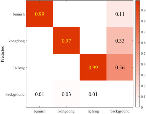
Figure 10. Confusion matrix of model training results.

Precision reflects the overall accuracy of the model in terms of target recognition and classification at the given iteration. A model prediction accuracy closer to 1 indicates superior performance. From the analysis of Figure 11a, it can be observed that the prediction accuracy of the model exhibits an overall upward trend as the number of iterations increases. When the number of iterations is small, the prediction accuracy of the model initially increases and then decreases, followed by oscillations without convergence as it continues to increase. As the number of iterations gradually increases, the model accuracy gradually stabilizes. When the number of iterations reached 200, the overall prediction rate reached 0.987. Figure 11b illustrates that as the number of model iterations increases, the recall rate exhibits an overall trend of initially rising rapidly, followed by fluctuations, and eventually stabilizing. When the number of iterations reaches 200, the final recall rate of the model reaches 0.969.

Figure 11

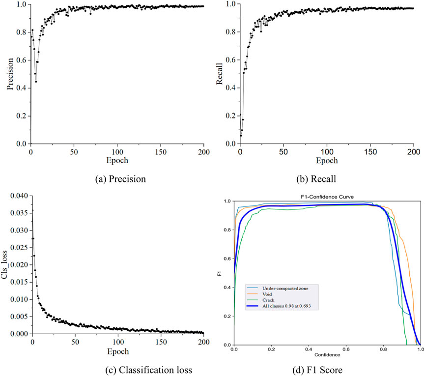
Figure 11. Model training results. (a) Precision (b) Recall. (c) Classification loss (d) F1 Score.

Classification loss refers to whether the model is correct in calculating the anchor box and the corresponding recognition category. As can be seen from Figure 11c, with the increase in the number of iterations, the model classification loss shows a tendency to decrease rapidly, and then the rate slows down and gradually converges to 0 (in the classification loss, a smaller the value means more accurate classification). When the iteration number reaches 200, the loss rate of the model reaches 2.97 × 10⁻⁴. F1 Score is the harmonic average of accuracy and recall rate, and its value ranges from 0 to 1. A higher score indicates a better prediction performance of the model. Figure 11d illustrates the variation of the F1 Score for different confidence thresholds. Based on the above analysis, as the confidence threshold gradually increases, the F1 Score exhibits a trend of initially increasing and subsequently decreasing. When the confidence threshold is around 0.2, the F1 Score reaches its maximum value and maintains this value until the confidence threshold increases to around 0.8. Although the model F1 Score decreases with the increase in confidence, the overall recognition performance remains satisfactory.

Based on the evaluation of the index results following the aforementioned model training, it is evident that the trained model is capable of accurately identifying the locations and categories of non-compactness, voids, and cracks in radar imaging of reconstructed and expanded roadbeds. Furthermore, the overall recognition accuracy achieves a high level of 98.7%.

5.4 Defect identification results

The GPR images of the roadbed junctions were preprocessed, followed by the application of the proposed target detection algorithm to identify and classify the geological radar images corresponding to the suspected roadbed defect sections.

Figure 12 illustrates the GPR image and recognition result of a void defect, where irregular curve features are consistent with electromagnetic wave propagation simulations. The optimized YOLOv5 model accurately marked the void boundaries, which closely matched the actual defect, and remained robust even with slight variations in burial depth. Figure 13 shows the imaging characteristics of a looseness defect, with clear reflections in the upper part and blurred signals in the lower part due to pore scattering and signal attenuation. The model successfully identified the looseness region, demonstrating good adaptability and tolerance to defects without clear geometric boundaries. Figure 14 presents the GPR image of a vertical crack, where typical convex hyperbolic reflections were observed. The model precisely delineated the crack distribution, highly consistent with the actual path, highlighting its high accuracy in detecting complex linear defects.

Figure 12

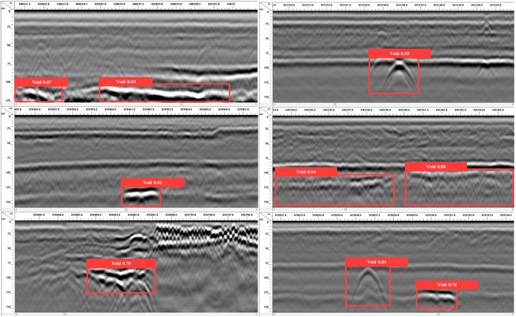
Figure 12. Void defect identification results.

Figure 13

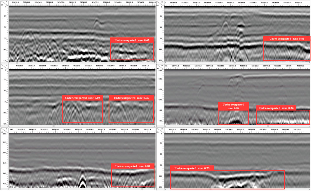
Figure 13. Non-compactness defect identification results.

Figure 14

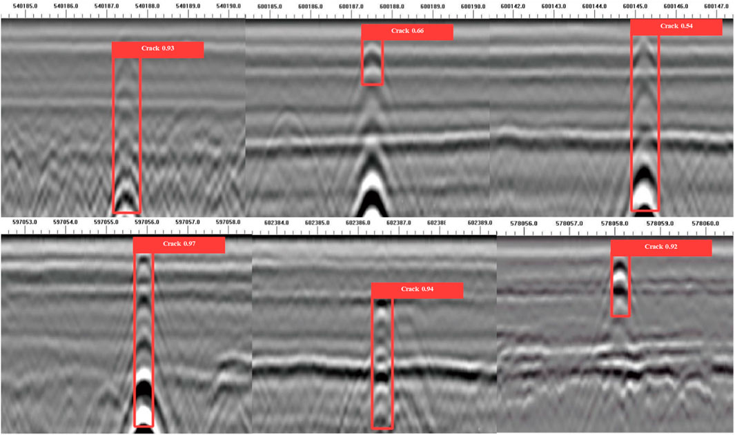
Figure 14. Crack defect identification results.

In summary, the proposed model can effectively locate and identify the voids, non-compactness, and cracks at the junction of the reconstructed and expanded roadbed. The recognition results of the three defect types are highly consistent with electromagnetic wave propagation patterns. This confirms the effectiveness and generalization capability of the proposed method across various defect forms and signal qualities, providing reliable support for the rapid screening of subgrade defects in practice.

This study aims to accurately identify typical defects at junctions of reconstructed and expanded expressway subgrades, including voids, looseness, and cracks. To this end, the optimized YOLOv5 was chosen as the core recognition algorithm due to its efficiency and adaptability in object detection. Adopting an end-to-end framework, it enables rapid dataset processing and result output, meeting practical requirements for fast defect screening. It also supports multi-class detection, allowing simultaneous identification of voids, looseness, and cracks without separate models for each type. The optimized YOLOv5 achieved recognition accuracies of 97%, 99%, and 99% for voids, looseness, and cracks, respectively, demonstrating high precision in multi-class defect detection.

The proposed method has been developed into a “simulation–field measurement–intelligent recognition” technical framework, offering a novel approach for defect detection and maintenance at roadbed junctions. It shows strong robustness and generalization: the dataset covers multiple defect types and integrates generalized simulation results from engineering cases with field measurements, capturing common features of real-world defects. YOLOv5 is trained on actual defect features, so its recognition logic is not limited to a single case.

Nevertheless, some limitations remain. Simplified model parameters, idealized defect morphologies, geological constraints of field data, and challenges in detecting small or deep-seated defects indicate areas for further improvement. Despite these, the method shows potential applicability in other practical cases with similar subgrade junction defects.

6 Conclusion

In view of the prevalent road defects in highway reconstruction and expansion projects, as well as the limited means and insufficient accuracy of existing internal defect detection methods, this paper focuses on identifying defects at the junction of reconstructed and expanded roadbeds. By integrating numerical simulation, field experiments, and deep learning techniques, the study investigates the application of target detection deep learning algorithms in GPR imaging for defect detection and identification at the reconstructed and expanded roadbed junction. The main conclusions are as follows:

1.The electromagnetic waves exhibit two sets of parallel convex hyperbolas within the circular cavity defects. The existence of non-compactness defects causes the overall reflected wave signal to display a distinct upper portion and a blurred lower portion in the imaging feature. Additionally, the electromagnetic waves show multiple nearly parallel convex hyperbolas in proximity to vertical cracks.

2.The type of defect can significantly influence the detection imaging effect. Specifically, defects located at different horizontal positions will only alter the horizontal position of the hyperbola in the imaging result without affecting the overall characteristics of the generated image features. The defects of different burial depths greatly influence the hyperbolic imaging effect. As the burial depth of the defect increases, the amplitude of the hyperbola decreases significantly. For the same defect at varying burial depths, the opening size of the hyperbola increases with increasing burial depth. This may lead to confusion between the hyperbolas generated by small-sized defects in the deep layer and those generated by large-sized defects in the shallow layer, potentially resulting in misjudgment.

3.The enhanced target recognition algorithm for junction defect detection, which is based on the YOLOv5 network, has achieved accuracy rates of 97% for cavity defect recognition, 99% for non-compactness defects, and 99% for crack defects.

Data availability statement

The raw data supporting the conclusions of this article will be made available by the authors, without undue reservation.

Author contributions

YR: Writing – original draft. YS: Writing – review and editing. GL: Writing – original draft. JL: Data curation, Formal Analysis, Writing – review and editing. KW: Funding acquisition, Investigation, Writing – original draft. CX: Conceptualization, Writing – review and editing.

Funding

The author(s) declare that financial support was received for the research and/or publication of this article. The authors acknowledge the financial support provided by the Training Program for Academic and Technical Leaders in Key Disciplines in Jiangxi Province, China - Leading Talent Project (20225BCJ22014), Science and Technology Project of Jiangxi Provincial Department of Transportation (2023C0005) and the Research and Innovation Program for Graduate Students in Chongqing (CYB240258).

Conflict of interest

Authors YR and YS were employed by Jiangxi Provincial Key Laboratory of Highway Bridge and Tunnel Engineering and Jiangxi Communications Investment Maintenance Technology Group Co., Ltd. Author JL was employed by Jiangxi Communications Investment Group Co., Ltd.

The remaining authors declare that the research was conducted in the absence of any commercial or financial relationships that could be construed as a potential conflict of interest.

Generative AI statement

The author(s) declare that no Generative AI was used in the creation of this manuscript.

Any alternative text (alt text) provided alongside figures in this article has been generated by Frontiers with the support of artificial intelligence and reasonable efforts have been made to ensure accuracy, including review by the authors wherever possible. If you identify any issues, please contact us.

Publisher’s note

All claims expressed in this article are solely those of the authors and do not necessarily represent those of their affiliated organizations, or those of the publisher, the editors and the reviewers. Any product that may be evaluated in this article, or claim that may be made by its manufacturer, is not guaranteed or endorsed by the publisher.

References

Abdelsamei, E., Sheishah, D., Runa, B., Balogh, O., Tóth, C., Primusz, P., et al. (2024). Application of ground penetrating radar in the assessment of aged roads: focus on complex structures under different weather conditions. Pure Appl. Geophys. 181 (12), 3633–3651. doi:10.1007/s00024-024-03604-y

CrossRef Full Text | Google Scholar

Amaral, L. C. M., Roshan, A., and Bayat, A. (2023). Automatic detection and classification of underground objects in ground penetrating radar images using machine learning. J. Pipeline Syst. Eng. Pract. 14 (4), 04023040. doi:10.1061/jpsea2.pseng-1444

CrossRef Full Text | Google Scholar

Bu, J., Jing, G., Long, X., Wang, L., Peng, Z., and Guo, Y. (2025). Intelligent classification of ballast bed defects using a bimodal deep learning model. Transp. Geotech. 50, 101464. doi:10.1016/j.trgeo.2024.101464

CrossRef Full Text | Google Scholar

Chi, Y., Pang, S., Mao, L., and Zhou, Q. (2024). Research on airborne ground-penetrating radar imaging technology in complex terrain. Remote Sens. 16 (22), 4174. doi:10.3390/rs16224174

CrossRef Full Text | Google Scholar

Geng, J., He, J., Ye, H., and Zhan, B. (2022). A clutter suppression method based on LSTM network for ground penetrating radar. Appl. Sci. 12 (13), 6457. doi:10.3390/app12136457

CrossRef Full Text | Google Scholar

Guo, L., Cai, L., and Chen, D. (2022). “Research on ground-penetrating radar denoising algorithm based on CEEMD and permutation Entropy[C]//2022 IEEE 6th advanced information technology,” in Electronic and automation control conference (IAEAC), 263–268. doi:10.1109/IAEAC54830.2022.9929797

CrossRef Full Text | Google Scholar

Guo, Y., Liu, G., Jing, G., Qu, J., Wang, S., and Qiang, W. (2023). Ballast fouling inspection and quantification with ground penetrating radar (GPR). Int. J. Rail Transp. 11 (2), 151–168. doi:10.1080/23248378.2022.2064346

CrossRef Full Text | Google Scholar

Kan, Q., Liu, X., Meng, A., and Yu, L. (2024). Intelligent recognition of road internal void using ground-penetrating radar. Appl. Sci. 14 (24), 11848. doi:10.3390/app142411848

CrossRef Full Text | Google Scholar

Li, Y. S., Du, Y. C., Liu, C. L., Yue, G. H., and Li, F. (2024). Adaptive curriculum learning for enhanced detection of Subsurface distress using ground penetrating radar. China J. Highw. Transp. 37 (12), 244–257. doi:10.19721/j.cnki.1001-7372.2024.12.007

CrossRef Full Text | Google Scholar

Ling, D., Zhao, Y., Wang, Y., and Huang, B. (2016). Study on relationship between dielectric constant and water content of rock-soil mixture by time domain reflectometry. J. Sensors 2016 (1), 1–10. doi:10.1155/2016/2827890

CrossRef Full Text | Google Scholar

Liu, W., Yang, X., Yan, Y., wang, H., Zhang, J., and Heikkilä, R. (2025). A state-of-the-art review on graph characterization and automated detection of road underground targets using ground-penetrating radar. Measurement 244, 116429. doi:10.1016/j.measurement.2024.116429

CrossRef Full Text | Google Scholar

Lv, G., Liu, J., Xie, Q., Wang, K., and Han, B. (2023). Rapid identification and location of defects behind tunnel lining based on ground-penetrating radar. J. Perform. Constr. Facil. 37 (4), 04023031. doi:10.1061/jpcfev.cfeng-3783

CrossRef Full Text | Google Scholar

Morris, I. M., Kumar, V., and Glisic, B. (2021). Predicting material properties of concrete from ground-penetrating radar attributes. Struct. Health Monit. 20 (5), 2791–2812. doi:10.1177/1475921720976999

CrossRef Full Text | Google Scholar

Park, C.-H., Behrendt, A., LeDrew, E., and Wulfmeyer, V. (2017). New approach for calculating the effective dielectric constant of the moist soil for microwaves. Remote Sens. 9 (7), 732. doi:10.3390/rs9070732

CrossRef Full Text | Google Scholar

Puntu, J. M., Chang, P.-Y., Lin, D.-J., Amania, H. H., and Doyoro, Y. G. (2021). A comprehensive evaluation for the tunnel conditions with ground penetrating radar measurements. Remote Sens. 13 (21), 4250. doi:10.3390/rs13214250

CrossRef Full Text | Google Scholar

Qinggang, W., and Xueming, Z. (2020). Remote sensing object detection via an improved YOLO network. Int. J. Perform. Eng. 16 (11), 1803. doi:10.23940/ijpe.20.11.p12.18031813

CrossRef Full Text | Google Scholar

Sonoda, J., and Nakamichi, K. (2024). A simple augmentation method using cutout for ground penetrating radar image in deep learning. IEICE Trans. Electron. E107 (11), 497–500. doi:10.1587/transele.2023ess0005

CrossRef Full Text | Google Scholar

Tang, J., Chen, C., Huang, Z., Zhang, X., Li, W., Huang, M., et al. (2022). Crack unet: crack recognition algorithm based on three-dimensional ground penetrating radar images. Sensors 22 (23), 9366. doi:10.3390/s22239366

PubMed Abstract | CrossRef Full Text | Google Scholar

Tešić, K., Baričević, A., and Serdar, M. (2021). Non-destructive corrosion inspection of reinforced concrete using ground-penetrating radar: a review. Materials 14 (4), 975. doi:10.3390/ma14040975

PubMed Abstract | CrossRef Full Text | Google Scholar

Tesic, K., Baricevic, A., Serdar, M., and Gucunski, N. (2022). Characterization of ground penetrating radar signal during simulated corrosion of concrete reinforcement. Automation Constr. 143, 104548. doi:10.1016/j.autcon.2022.104548

CrossRef Full Text | Google Scholar

Wagner, N., Emmerich, K., Bonitz, F., and Kupfer, K. (2011). Experimental investigations on the Frequency- and temperature-dependent dielectric material properties of soil. IEEE Trans. Geoscience Remote Sens. 49 (7), 2518–2530. doi:10.1109/tgrs.2011.2108303

CrossRef Full Text | Google Scholar

Wang, T., Zhang, W., Li, J., Liu, D., and Zhang, L. (2024). Identification of complex slope subsurface strata using ground-penetrating radar. Remote Sens. 16 (2), 415. doi:10.3390/rs16020415

CrossRef Full Text | Google Scholar

Wanyan, J. F., Jiang, Y. X., Xu, X. L., Chang, M., and Huang, Y. (2024). Defect recognition method of urban underground pipe NetworkBased on improved YOLOv5 algorithm. Comput. Meas. and Control 32 (11), 258–264. doi:10.16526/j.cnki.11-4762/tp.2024.11.036

CrossRef Full Text | Google Scholar

Xu, H., Yan, J., Feng, G., Jia, Z., and Jing, P. (2024). Rock layer classification and identification in ground-penetrating radar via machine learning. Remote Sens. 16 (8), 1310. doi:10.3390/rs16081310

CrossRef Full Text | Google Scholar

Yu, M. M., Zhang, Y., Chen, T., and Xu, Z. (2023). Identification and evaluation of hidden diseases in pavements based on 3D ground penetrating radar. Highway 68 (3), 383–388.

Google Scholar

Zhang, S. T., Ren, X. H., Yang, L. X., and Ge, D. B. (2011). A novel method of object bistatic RCS based on FDTD methodand its application. J. microwaves. 27 (3), 5–9. doi:10.14183/j.cnki.1005-6122.2011.03.001

CrossRef Full Text | Google Scholar

Zhang, H. R., Wang, G. F., and Zhang, F. Q. (2018). Early roadway disease detection based on ground-penetrating radar signal band dielectric spectral characteristics. Sci. Technol. Eng. 18 (4), 344–348.

Google Scholar

Zhang, T., Zhang, D., Zheng, D., Guo, X., and Zhao, W. (2022). Construction waste landfill volume estimation using ground penetrating radar. Waste Manag. and Res. J. a Sustain. Circular Econ. 40 (8), 1167–1175. doi:10.1177/0734242x221074114

PubMed Abstract | CrossRef Full Text | Google Scholar

Zhang, J. H., Zhang, A. S., Peng, J. H., Li, J., Luo, J. H., and Xie, T. X. (2024). Permanent deformation of highway subgrade under long-term cyclic loading: a review. China J. Highw. Transp. 37 (11), 1–25. doi:10.19721/j.cnki.1001-7372.2024.11.001

CrossRef Full Text | Google Scholar

Zhou, N., Tang, J., Weixiong, L., Huang, Z., and Xiaoning, Z. (2023). Application of clustering algorithms to void recognition by 3D ground penetrating radar. Front. Mater. 10, 1239263. doi:10.3389/fmats.2023.1239263

CrossRef Full Text | Google Scholar