Data-driven progress prediction in construction: a multi-project portfolio management approach

Introduction: Construction projects often experience delays and cost overruns, particularly in regions like New Zealand, where natural hazards and climate change exacerbate these risks. Despite extensive research on forecasting overall construction timelines, limited attention has been given to stage-wise progress across the project lifecycle, constraining project managers’ ability to monitor performance and respond to risks.

Methods: To address this gap, the study develops a stage-based forecasting model using Multinomial Logistic Regression, which was identified as the most suitable method after comparison with selected machine learning approaches within the study’s scope and assumptions. A stepwise comparative framework was employed to assess combinations of duration, value, type, and contractor involvement, measuring accuracy, log-loss, and Cohen’s kappa using 10 years of New Zealand construction data. Model reliability was further examined using confusion matrices to derive sensitivity, specificity, predictive values, and balanced accuracy. Validation was conducted through cross-validation, ROC/AUC, and temporal hold-out testing.

Results: The results show that while all models performed reasonably well, the model using only project duration and value achieved the highest accuracy. The validation procedures confirmed the framework’s robustness and generalisability. Visualisations further illustrated milestone-specific progress predictions (5%–100%), making stage-wise forecasts easy to interpret.

Discussion: The model provides project managers with practical insights for planning, monitoring, risk management, and resource allocation. By offering a transparent and interpretable approach, it bridges statistical forecasting with real-world practice, supporting timely delivery and data-driven infrastructure development. Future research could incorporate additional factors, extend the model locally and internationally, and explore integration with digital twins or real-time adaptive systems.

1 Introduction

Construction projects are inherently dynamic and complex and are subject to numerous uncertainties that can significantly impact their performance (Adamtey and Kereri, 2023; Kazar and Küçük, 2024). These uncertainties often result in cost and time overruns, influenced by both internal and external factors (Assaad et al., 2020; Kerzner, 2022). Internal factors, such as poor management, inadequate leadership, conflicts among project parties, and technical issues like design changes, further contribute to time and cost overruns (Egwim et al., 2021; Gamil and Abdul Rahman, 2020; Ismaila et al., 2022). External factors such as financial constraints, political instability, and economic fluctuations, along with unforeseen events like the COVID-19 pandemic, natural disasters, and climate change, disrupt project delivery by significantly impacting schedules and budgets (Alsulamy, 2025; Durdyev and Hosseini, 2020; Ingle et al., 2021; Klingsad and Ayudhya, 2025).

In New Zealand, where the construction sector is highly exposed to climate-related and environmental risks, performance disruptions become more frequent and severe, compounding the impacts of financial, political, and global uncertainties (Alboğa et al., 2025; Boudreaux et al., 2023; Ingle and Mahesh, 2024; Tagharobi et al., 2024). These risks underscore the need for reliable forecasting tools to support planning, time management, and proactive progress monitoring, thereby mitigating disruptive effects, delays, and cost overruns (Bertram et al., 2019; Fakunle and Fashina, 2020).

In response, various control systems and techniques have been developed to help project managers assess deviations from planned time and cost benchmarks (Assaad et al., 2020; Klingsad and Ayudhya, 2025). However, most existing methods tend to emphasise overall project performance in their forecasting approaches rather than providing stage-specific predictions that reflect project characteristics and uncertainties (Lalmi et al., 2025; Székely et al., 2025). For example, the S-curve technique provides only a cumulative perspective of progress and lacks milestone-level granularity. Earned Value Management (EVM), though widely applied, depends heavily on baseline accuracy and detailed task-level inputs, making it complex and less reliable in dynamic environments (Proaño-Narváez et al., 2022). Risk Management (RM) frameworks rely on subjective judgment and remain static, with limited integration into stage-wise forecasting (Ingle and Mahesh, 2024). Machine learning (ML) methods have been explored, but their “black-box” nature restricts interpretability and practical adoption (Carvalho et al., 2019). Other techniques, such as bottom-up models or hybrid frameworks, also face challenges of impractical data requirements and limited applicability (Anand et al., 2023).

These shortcomings underscore the need for stage-based forecasting approaches that are both practical and interpretable, bridging the gap between statistical modelling and real-world implications while supporting adaptive decision-making tools. Considering these challenges, this study seeks to address the following research questions:

• To what extent can project characteristics explain progress and advancement at each stage of a construction project?

• How can project progress be accurately forecast at different stages, and how can this support effective monitoring and risk mitigation in the construction industry?

To address current limitations in construction progress forecasting and respond to the research questions, this study adopts a multiphase comparative modelling approach using Multinomial Logistic Regression (MLR), within the project’s assumptions and scope. MLR was selected after comparison with alternative machine learning methods, as it offers a balance of interpretability and predictive performance. Building on this, the study examines the relationship between project progress and key input variables—such as duration, value, type, and contractor involvement. Several model configurations are tested through a stepwise framework to evaluate predictive accuracy, robustness, and generalisability. Finally, the results are visualised through milestone-specific forecasts (5%–100%), providing project managers with transparent and interpretable insights to support planning, monitoring, risk management, and resource allocation.

The proposed framework extends this contribution by offering a structured approach to forecasting project progress across the construction lifecycle, delivering timely insights to optimise resources and mitigate delays and deviations. Although developed using New Zealand data, the model is adaptable to countries with similar contexts and can be transferred to other industries by incorporating local data, thereby increasing its broader relevance across the global construction sector. By leveraging core variables such as project value and duration, available in virtually any context, it establishes a transparent and replicable tool that supports resilient, efficient, and sustainable practices.

To guide the reader, this paper is organised into eight sections. Section 1 introduces the research context and objectives. Section 2 reviews the relevant literature on construction progress and forecasting challenges. Section 3 outlines the methodology employed in the study. Section 4 presents the results and key analytical insights. Section 5 discusses the findings in relation to previous research, and Section 6 highlights the study’s limitations. Section 7 outlines the practical and theoretical contributions. Finally, Section 8 concludes the paper and suggests directions for future research. This structured approach enhances understanding of progress dynamics and supports more accurate, data-driven decision-making across the construction project lifecycle.

2 Literature review

Accurate planning and progress prediction are essential for minimising delays, controlling costs, and enhancing project efficiency (Johansen et al., 2025; Sovacool and Ryu, 2025). In contrast, poor planning often leads to resource mismanagement, budget overruns, and project delays (Castañeda et al., 2025; Sheikhkhoshkar et al., 2025). Contributing factors include planning deficiencies, poor scheduling, inadequate site management, contractor inexperience, payment delays, and underestimated costs (Abdallah et al., 2024; Castañeda et al., 2025). Additionally, unmanaged project complexity significantly increases the risk of failure (Ahmadzai and Ye, 2025; Daoud et al., 2023; Jiang et al., 2025). Beyond technical factors, management practices such as strong leadership, effective collaboration, and structured planning can improve performance, yet institutional inefficiencies and organisational barriers often undermine successful delivery (Castañeda et al., 2025; Koirala and Shahi, 2024).

In response, various methods have been developed to assess and predict the progress of construction projects across their lifecycle. However, most existing studies focus on overall forecasting, which estimates the final project duration and evaluates performance only at completion. Moreover, task-level techniques require detailed input, making them complex and less reliable in dynamic environments. While both approaches are useful for long-term planning, they overlook the need to forecast progress at intermediate stages (e.g., 30%, 50%, 90%). Within these categories, overall forecasting and task-level approaches, two widely adopted methods are $EVM$ and $RM$ (Assaad et al., 2020; Ingle and Mahesh, 2024).

$EVM$ integrates schedule, scope, and resource metrics to monitor progress and identify deviations, using key indicators such as $PlannedValue\left(PV\right)$, $EarnedValue\left(EV\right)$, and $ActualCost\left(AC\right)$. These core metrics, outlined in Table 1, enable the evaluation of both schedule and cost performance. In contrast, $RM$ focuses on the stochastic nature of construction activities, assessing the potential impact of unforeseen events and recommending mitigation strategies. While $EVM$ relies on historical data to project future performance trends, RM emphasises proactive risk identification and control (Assaad et al., 2020; Proaño-Narváez et al., 2022).

Table 1

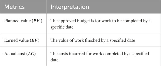
Table 1. Basic EVM metric.

Despite their widespread use, both EVM and RM have notable limitations. EVM relies on monetary units rather than time, which can lead to misleading conclusions (Ngo et al., 2022; Picornell et al., 2017; Stone, 2023). RM faces challenges in accurately predicting and quantifying the impact of unforeseen events, as it depends on assumptions about risk probabilities and outcomes, which may be overly simplistic or inaccurate (Ballesteros-Pérez and Elamrousy, 2018; Ballesteros-Pérez et al., 2020b). Moreover, the limited awareness and adoption of EVM among construction professionals further restrict its practical effectiveness (Keng and Shahdan, 2015).

Nonetheless, EVM has been successfully applied in several studies. Nadafi et al. (2019) used EVM to forecast time and cost outcomes, while Picornell et al. (2017) adapted it for unit-price contracts, enhancing decision-making. Similarly, Anwar et al. (2024) demonstrated its effectiveness in evaluating cost and time performance in public construction projects. Comparative studies provide further insights, particularly where researchers have examined EVM extensions through the integration of alternative methods. For example, Colin and Vanhoucke (2015) compared extensions of EVM and found that EVM-SNB (Subnetwork Buffers) achieved 80% accuracy with only 25% control effort. In comparison, EVM-FPB (Feeding Path Buffers) reached 83% efficiency with 43% effort—both outperforming traditional EVM-LPB at lower resource costs. Similarly, Ngo et al. (2022) reformulated EVM using singularity functions (SF), enabling continuous progress tracking and more accurate estimates than conventional discrete models. Combining EVM with PERT has also been shown to improve the forecasting accuracy of duration and cost (Anwar et al., 2024; Ballesteros-Pérez et al., 2020a; Ballesteros-Pérez et al., 2020b; Getawa Ayalew and Ayalew, 2024). Collectively, these studies demonstrate that while enhanced EVM variants can improve performance, they remain constrained by their reliance on monetary metrics rather than time-based measures of progress.

Mathematical models offer an alternative approach (Alsaedi and Naimi, 2024; Dattadean, 2016; Ghoroqi et al., 2023; Kumar and Mouli, 2018). For example, Ballesteros-Pérez et al., 2020a proposed formulas to estimate average project duration ($\mu p$), achieving up to 64% improvement in MAE and 90% in MSE compared to PERT. Compared to EVM-based extensions, these models explicitly integrate time variables; however, they still lack flexibility for dynamic, milestone-specific monitoring.

In contrast to purely overall forecasting methods, several statistical models integrate contextual variables to capture how project-specific dynamics shape construction performance (Mohammadjafari et al., 2024; Morozovskiy et al., 2019; Rudeli et al., 2017; Yousefi et al., 2019). For example, Chao and Chen (2015) used S-curve modelling incorporating factors such as project simplicity, team competence, contract amount, duration, type of work, and location. Their model achieved a mean RMSE of 0.027 and a maximum RMSE of 0.047, with a correlation of 0.65 between the number of contracts and project duration. Similarly, Cao et al. (2015) examined Building Information Modelling (BIM) practices using linear and hierarchical regression, identifying project size and type as significant predictors of BIM effectiveness. Project size showed a significant positive influence on task efficiency (TEY) and overall BIM success (OBS), with R² values of 0.165 for TEY and 0.075 for OBS, respectively. The highest R² value reached 0.339, highlighting the role of BIM use and client support. Olanipekun et al. (2018) employed Confirmatory Factor Analysis (CFA) and Structural Equation Modelling (SEM) to investigate the impact of motivation and owner commitment on green building project performance. Both models showed good fit (e.g., $RMSEA=0.055-0.058$; $CFI=0.965-0.967$). Assaad et al. (2020) developed a framework to predict project cost and schedule by assessing 25 key risks, using expert surveys and modelling validated through a case study. Other studies also reinforce these findings, Picornell et al. (2017), Alaloul et al. (2016), and Ackon et al. (2025) emphasised the role of contractor count, while Santolini et al. (2021), Sekar et al. (2021) and Azmat and Siddiqui (2023) highlighted project size, and Ramli et al. (2018) focused on project type in construction performance. Additionally, advanced models have been developed to improve forecasting accuracy. Yilmaz (2020) developed a multivariate non-linear delay estimation model, while Kim et al. (2019) used multiple regression to estimate construction durations with 88.51% accuracy. Collectively, these studies demonstrate that contextual variables such as size, type, and contractor count enhance the explanatory power of forecasting models. Compared with traditional methods like EVM, statistical models provide greater predictive depth by accounting for project-specific and contextual factors; however, their accuracy remains modest relative to machine learning approaches.

Building on statistical foundations, other advanced frameworks have been introduced to improve project monitoring and forecasting. Alizadehsalehi and Yitmen (2016) integrated field data capturing technologies (FDCT) with BIM to automate construction project progress monitoring (ACPPM). Using the Relative Importance Index (RII), their study found 3D Laser Scanning most effective, with RII values of 0.89 for physical data collection and 0.86 for progress visualisation. Similarly, Assaad et al. (2020) proposed a comprehensive framework for evaluating project progress, predicting cost and time, and assessing construction risks using distribution functions and survey-based risk scoring.

Compared with regression and statistical models, machine learning (ML) and deep learning (DL) methods have achieved notable gains in forecasting accuracy for construction progress and costs (Akinosho et al., 2020; Al-Ghzawi and El-Rayes, 2024; de Sá Pedroso, 2017; Liben et al., 2024; Merdžanović et al., 2023; Regona et al., 2022a; 2022b; Yu et al., 2022). For instance, Guo et al. (2019) demonstrated that Wavelet Neural Networks (WNN) reduced MAPE by 78% with $R2=0.66$ compared with regression ($R2=0.475$), although requiring large datasets and offering limited interpretability. Jaber et al. (2020) developed regression-based ML models to predict SPI, CPI, and TCPI using six inputs, achieving R² values of 73.2%, 79.6%, and 74.4%, respectively, outperforming traditional statistical models. Ensemble approaches have also proven superior. Egwim et al. (2021) reported 76% accuracy in delay prediction by combining Decision Trees, Random Forests, and Naïve Bayes. More advanced comparisons by Alsulamy, (2025) revealed that LGBM outperformed $CatBoost$ and $XGBoost$ across all time-overrun levels, while $GAN$ (91% accuracy) surpassed LSTM (88%) and MLP (83%) (Alsulamy, 2025). These findings highlight the comparative advantage of ML/DL methods over regression-based and $EVM$ approaches, though challenges such as the “black box” problem, high computational demands, and ethical concerns continue to limit their adoption (Akinosho et al., 2020; Burrell, 2016; Regona et al., 2022b).

Alternative approaches, including Delphi techniques, chance-constrained programming, and System Dynamics (SD), provide additional perspectives but lag behind ML in predictive accuracy and adaptability. Alaloul et al. (2016) ranked coordination factors affecting building project performance using the Delphi method, but it is prone to expert bias and groupthink. Sun et al. (2023) applied chance-constrained programming to minimise delays under uncertainty, yet such models often rely on idealised assumptions and extensive calibration.

Some researchers have also applied System Dynamics (SD) to estimate construction project performance (Al-Gahtani et al., 2022; Bajomo et al., 2022; Ding et al., 2016; Leon et al., 2018; Taha et al., 2022). Leon et al. (2018) developed an SD model for road projects, integrating cost, schedule, quality, and other performance metrics. While effective in forecasting and scenario analysis, the model’s accuracy may be limited by assumptions and simplified dynamics. Thiele et al. (2025) introduced NPMB, achieving 95.6% accuracy in predicting schedule trends but only 48.9% for cost. However, it highlights trend bias rather than stage-specific progress probabilities.

Taken together, existing models reveal a clear comparative pattern. EVM lacks time integration and, although built on task-level planning data, reduces activity progress into aggregated cost-based measures that obscure detailed scheduling dynamics. RM depends on rigid risk assumptions and faces challenges in predicting and quantifying the impact of unforeseen events, as its probability-based inputs are often simplistic or inaccurate. The S-curve technique offers only a cumulative perspective of progress and lacks the milestone-level granularity necessary for proactive monitoring, thereby limiting its usefulness. ML and DL approaches consistently outperform traditional methods in predictive accuracy, yet they struggle with interpretability and often function as black-box systems. SD-based approaches, while valuable for mapping systemic interactions and resource flows, tend to oversimplify the complexity of real-world projects. Statistical models enhance explanatory depth by integrating contextual variables, but they tend to plateau in accuracy compared to advanced AI-based methods.

Critically, these diverse approaches emphasise overall completion forecasting, with limited attention to stage-specific progress. These limitations highlight the need for an approach that integrates statistical transparency and stage-specific accuracy with broad applicability and practical relevance. Such an approach should provide milestone-level insights without the opacity of black-box models or the heavy data requirements of task-level methods. The present study addresses this gap by introducing an interpretable, probabilistic framework designed to generate stage-based forecasts that support proactive planning, resource allocation, and monitoring in construction projects.

3 Research methodology

This study employs a multi-step methodology, illustrated in Figure 1, to develop and validate a probabilistic, stage-based forecasting model for construction progress. The process began with data preparation and preprocessing, followed by correlation analysis to examine relationships among predictors. A modelling framework was then established, and candidate models—including ML approaches and MLR were compared, with MLR identified as the most suitable technique. Subsequently, stepwise MLR fitting was conducted by progressively introducing variables and interaction terms to determine the optimal specification. Model performance was evaluated using accuracy, kappa, AIC, and log-loss, while class-level metrics such as sensitivity, specificity, PPV, NPV, and balanced accuracy were applied to assess reliability. Finally, validation was performed through cross-validation and temporal hold-out testing. The resulting optimal model provides practical implications for construction progress forecasting and supports data-driven decision-making.

Figure 1

Figure 1. Research methodology flowchart.

3.1 Data source and preprocessing

This study draws on a comprehensive dataset of over 220,000 construction projects undertaken in New Zealand between 2013 and 2022, encompassing both small- and large-scale developments. The dataset, sourced from Pacifica Company and supplemented with industry benchmarks, includes detailed information on project types, timelines, value estimates, contractors, progress, and locations. To ensure reliability and accuracy, several preprocessing steps were undertaken. After excluding incomplete records for key explanatory variables, less than 1% of cases were removed, resulting in a final analytical sample of approximately 218,000 projects. Project timelines were reformatted into a consistent date structure, enabling the accurate calculation of durations and progress intervals. Project value was normalised within each type (e.g., Civil, Residential, Commercial) using z-score standardisation, calculated as $Z=\left(x-\mu \right)/\sigma$. This transformation ensured a mean of zero and a standard deviation of one within each group, preserving relative differences while improving comparability across categories and reducing the impact of large value ranges. In contrast, variables such as duration, project type weight, and number of contractors exhibited limited variability and did not require transformation. Categorical variables were harmonised to resolve inconsistencies in labelling, and outliers were reviewed to minimise the influence of erroneous entries. These steps established a consistent, standardised dataset suitable for robust model development.

3.1.1 Definitions

Project progress ($\mathit{p}\mathit{p}$) represents the percentage of a project completed at a given time, categorised into seven levels: 5%, 15%, 30%, 50%, 70%, 90%, and 100%, where 5% indicates project initiation and 100% represents completion. Here, pp is a dependent variable and is modelled as a function of several independent variables: project value ($\mathit{p}\mathit{v}$), duration ($\mathit{d}\mathit{u}$), project type, number of main contractors ($\mathit{n}\mathit{o}\mathit{c}$), and the interaction between time and value. Project value ($\mathit{p}\mathit{v}$) refers to the initial estimated value for construction, indicating project size and scale. Project type ($\mathit{p}\mathit{t}$) is classified into eight categories: Residential, Commercial, Industrial, Civil, Health, Education, Sport, and Heavy Industry/Energy, with a weight ($\mathit{w}\mathit{t}\mathit{p}$) assigned to each type based on its total value relative to all projects. The number of main contractors ($\mathit{n}\mathit{o}\mathit{c}$) reflects the total number of primary contractors involved in each project, serving as an indicator of the workforce scale. Duration ($\mathit{d}\mathit{u}$) captures the time in years since the project’s initiation, based on recorded progress intervals. This time factor is essential for understanding how duration influences project advancement and is integral to the performance modelling approach adopted in this study.

3.2 Correlation analysis

Examining the relationships between pp and variables such as du, $pv$, $wtp$, and $noc$ is essential for identifying key drivers and ensuring model accuracy. Pearson correlation is used to assess the linear relationships between these continuous variables, with the coefficient r calculated as:

$r=\frac{\sum \left(x-\overline{x}\right)\left(y-\overline{y}\right)}{\sqrt{\sum {\left(x-\overline{x}\right)}^2\sum {\left(y-\overline{y}\right)}^2}}(1)$

Where $x$ and $y$ are the variables and $\overline{x}$ and $\overline{y}$ are respectively the means of these variables. Correlation significance is assessed using a p-value; values below 0.05 indicate statistical significance.

3.2.1 Conditional correlation

As project progress is influenced by both time and project value, conditional correlation is used to isolate the effect of time while controlling the effect of project value. This approach clarifies how time alone impacts progress, independent of project size or budget.

$Correlation\left(projectprogressandduration|projectvalue\right)=r\left(pp\&du|pv\right)(2)$

3.3 Model framework

3.3.1 Candidate models

To predict $pp$, $MLR$ was selected as the primary model due to its interpretability, statistical rigour, and suitability for handling multiple outcome categories. $du$ and $pv$ were specified as the core explanatory variables, as they capture the temporal and financial dimensions most relevant to project outcomes. To benchmark the performance of MLR and ensure the robustness of model selection, alternative ML approaches were also considered, namely, Decision Trees and Random Forests. These models were selected to provide complementary perspectives: Decision Trees offer a simple, rule-based structure that can capture non-linear relationships, while Random Forests aggregate multiple trees to improve predictive accuracy and reduce variance.

The comparison across candidate models was conducted using $Accuracy$ and $hen’sKappa$ $\left(k\right)$. In this context, $Accuracy$ refers to the proportion of project progress stages correctly predicted by the model relative to the observed stages in the dataset, and it was measured from the confusion matrix by dividing the number of correct classifications by the total number of predictions. Cohen’s Kappa ($k$), in contrast, measures the level of agreement between predicted and actual classifications after adjusting for agreement expected by chance, and it was calculated by comparing the observed accuracy ($p_o$) with the expected accuracy ($p_e$) derived from the marginal totals of the confusion matrix. The formulas for Accuracy and Kappa are presented below.

$Accuracy=\frac{NumberofCorrectPredictions}{TotalPredictions}(3)$

$k=\frac{p_o-p_e}{1-p_e}(4)$

3.3.1.1 Model specification: multinomial logistic regression (MLR)

MLR is an extension of the logistic regression (LR) model, specifically designed for discrete variables with more than two levels (Liang et al., 2020; Ramadhan et al., 2017). Introduced by Luce (1959), this method has been widely applied across various fields, including the construction industry (Lin et al., 2014). In MLR, the dependent variable has $r+1$ possible outcomes; outcomes are denoted as $0,1,2,...,r,$ where $r>1$. One of these outcomes is chosen as the reference outcome, and $r$ pairwise logistic regressions are conducted between the reference outcome and the other outcomes. A binary logistic regression for the $h-th$ outcome, assuming zero as the reference event, can be defined using the following equation: $p_{ih}$ represents the probability that the $ith$ sample is associated with the $h-th$ outcome (El-Habil, 2012; Lin et al., 2014).

$\log it\left(P_{ih}\right)=\mathit{ln}\frac{P_{ih}}{P_{i0}}=b_{0h}+b_{1h}{x}_{i1}+b_{2h}{x}_{i2}+...+b_{kh}{x}_{ik}={\displaystyle \sum _{j=0}^k}{b}_{jh}{x}_{ij}(5)$

By taking the exponential of both sides of the log-odds formulation, the probability ratio is obtained as shown in Equation 6.

$\Rightarrow \frac{P_{ih}}{P_{i0}}=\mathit{exp}\left({\displaystyle \sum _{j=0}^k}{b}_{jh}{x}_{ij}\right)(6)$

Let $z_{ih}=\mathit{exp}\left({\displaystyle {\sum }_{j=0}^k}{b}_{jh}{x}_{ij}\right)$, therefore $z_{i\mathrm{h}}=\frac{p_{i\mathrm{h}}}{p_{i0}}$

To simplify the notation, we define as the exponential transformation of the linear predictor, as expressed in Equation 7.

$1={\displaystyle \sum _{t=0}^r}{p}_{it}=p_{i0}+{\displaystyle \sum _{t=1}^r}{p}_{it}=p_{i0}+{\displaystyle \sum _{t=1}^r}{p}_{i0}{z}_{ih}=p_{i0}\left(1+{\displaystyle \sum _{t=1}^r}{z}_{ih}\right)(7)$

Rearranging the expression for the baseline probability yields the closed-form solution presented in Equation 8.

$\Rightarrow p_{i0}=\frac{1}{\left(1+{\displaystyle {\sum }_{t=1}^r}{z}_{ih}\right)}=\frac{1}{1+\mathit{exp}\left({\displaystyle {\sum }_{j=0}^k}{b}_{jh}{x}_{ij}\right)}(8)$

Substituting the baseline term into the class-specific probability gives the multinomial logistic probability function, shown in Equation 9.

$\Rightarrow p_{ih}=\frac{{\displaystyle {\sum }_{t=1}^r}{z}_{ih}}{\left(1+{\displaystyle {\sum }_{t=1}^r}{z}_{ih}\right)}=\frac{\mathit{exp}\left({\displaystyle {\sum }_{j=0}^k}{b}_{jh}{x}_{ij}\right)}{1+\mathit{exp}\left({\displaystyle {\sum }_{j=0}^k}{b}_{jh}{x}_{ij}\right)}(9)$

When the response variable consists of only two outcomes, the model follows the binomial distribution. However, when the response variable has more than two outcomes, as in this study, the model follows the multinomial distribution (El-Habil, 2012; Liang et al., 2020). In this study, the MLR model is used to predict the probability of $pp$ from the initial phase to completion while considering factors such as $du,pv,noc,$ and $wtp$. According to the available data set, the pp is divided into seven levels: 5%–100%. These progress levels are symbolically associated with probabilities denoted as $P_{5\%}$, ${P_{15\%},P}_{30\%}$, $P_{50\%}$, $P_{70\%}$, $P_{90\%}$ and $P_{100\%}$ $.$ The outcome of project progress is defined across seven levels, with the initial phase (5%) serving as the reference level.

3.3.2 Stepwise model development and selection

After identifying the best candidate model based on the results in Section 3.3.1, the next step involved stepwise development to progressively add variables and interaction terms to find the optimal model. Variables were added stepwise based on their importance and correlation with project progress. The process began by testing $pv$ and $du$ separately, then together, followed by their interaction term. Next, $noc$ was added, and finally $wtp$ in the following specifications:

• $\mathit{M}\mathit{o}\mathit{d}\mathit{e}\mathit{l}1:pp\sim pv$

• $\mathit{M}\mathit{o}\mathit{d}\mathit{e}\mathit{l}2:pp\sim du$

• $\mathit{M}\mathit{o}\mathit{d}\mathit{e}\mathit{l}3:pp\sim du+pv$

• $\mathit{M}\mathit{o}\mathit{d}\mathit{e}\mathit{l}4:pp\sim du+pv+du*pv$

• $\mathit{M}\mathit{o}\mathit{d}\mathit{e}\mathit{l}5:pp\sim du+pv+noc$

• $\mathit{M}\mathit{o}\mathit{d}\mathit{e}\mathit{l}6:pp\sim du+pv+noc+wtp$

Model performance was evaluated using Accuracy, Residual Deviance, AIC, Log-Loss, and Cohen’s Kappa. Lower Residual Deviance, AIC, and Log-Loss indicated a better fit, while higher Accuracy and Kappa reflected stronger predictive power. The specification with the best overall performance across these metrics was selected as the optimal model. By forecasting progress at key milestones ($5\%-100\%$), the final model provides actionable insights for project managers, supporting more effective planning, risk management, and resource allocation.

3.3.3 Optimal model and predictive formula

Once the best specification was identified, the estimated coefficients were evaluated at a $0.05$ significance level to determine their statistical relevance. Statistically significant coefficients indicate the strength and direction of each factor’s contribution to predicting project progress. The final MLR model was then used to generate probability estimates for each progress milestone, with the predictive formula (Equations 1 – 5) applied to estimate the likelihood of reaching stages from 5% to 100%.

3.3.4 Optimal model performance in class-level diagnostic

The predictive performance of the optimal model was evaluated using the confusion matrix and a set of derived classification metrics. The confusion matrix compares predicted project progress stages against the observed stages, providing the foundation for quantifying both correct and incorrect classifications across categories. From this matrix, several metrics were calculated to capture different dimensions of model performance, including Accuracy, Sensitivity, Specificity, Precision (Positive Predictive Value, $\mathrm{P}\mathrm{P}\mathrm{V}$), Negative Predictive Value ($\mathrm{N}\mathrm{P}\mathrm{V}$), and Balanced Accuracy.

Sensitivity, shown in Equation 10, reflects the model’s ability to correctly identify projects in a given progress stage, whereas Specificity, defined in Equation 11, indicates the ability to correctly exclude non-cases. Precision (PPV), presented in Equation 12, measures the proportion of correct positive predictions, while NPV, given in Equation 13, quantifies the proportion of correct negative predictions. Balanced Accuracy, computed as the average of Sensitivity and Specificity, provides a more robust measure in the presence of class imbalance.

In addition, Odds Ratios $\left(OR=\mathit{exp}\left(\beta \right)\right)$ derived from the MLR coefficients were used to evaluate the relative influence of each predictor. Higher $OR$ values indicate stronger effects of the corresponding predictor on project progress. Together, these measures provide a comprehensive assessment of the model’s predictive capability, ensuring that evaluation accounts for both overall correctness and stage-level reliability.

$Sensitivity=\frac{TruePositives}{TruePositives+FalseNegatives}(10)$

$Specificity=\frac{TrueNegatives}{TrueNegatives+FalsePositives}(11)$

$PositivePredictiveValue=\frac{TruePositives}{TruePositives+FalsePositives}(12)$

$NegativePredictiveValue=\frac{TrueNegatives}{TrueNegatives+FalseNegatives}(13)$

3.4 Model validation

A two-stage validation strategy was employed to assess model reliability and minimise overfitting. First, a 5-fold stratified cross-validation was conducted on the training subset (projects commencing before 2019), ensuring the distribution of progress classes was preserved. At each iteration, four folds were used for model estimation and one for validation, and the process was repeated until all folds had served as validation. Final performance metrics were obtained by averaging across folds. To further evaluate estimate stability, models were tested under varying regularisation settings (decay parameters of 0, 0.01, and 0.10). Second, to approximate a real-world forecasting scenario, a temporal hold-out evaluation was conducted using projects commencing in 2019 or later. This separation ensured that the test set was temporally distinct from the training set, thereby allowing assessment of model generalisability under changing industry conditions. Together, these complementary approaches provide both resampling-based internal validation and independent temporal testing, strengthening the robustness of the modelling framework.

3.5 Practical implications

The optimal model is applied to real-world data from New Zealand’s construction industry to predict project progress across key milestones (5%–100%). It assesses how key factors influence progress over time, helping project managers anticipate challenges, optimise resources, and mitigate risks. By providing stage-specific insights, the model facilitates informed decision-making and proactive performance monitoring, making it a practical tool for enhancing project delivery and mitigating delays and cost overruns.

4 Findings and analysis

4.1 Data overview

Table 2 summarises New Zealand construction projects from 2013 to 2022, highlighting key statistics by project type. Residential projects dominate, comprising 68% of total projects, 39% of total value, and 201,503 contractors. Civil and commercial projects each account for 11% of projects, with civil projects contributing 24% of the value and employing 53,030 contractors, and commercial projects contributing 16% of the value and employing 55,044 contractors. Educational and industrial projects account for 5% and 3% of projects, with 4% and 5% of value, respectively. Sports and health projects each represent 1% of total projects, with value shares of 1% and 2%, and around 5,900 contractors each. The wtp column shows each type’s financial weight, while $noc$ highlights workforce distribution. This overview highlights the construction sector’s diversity in terms of scale, cost, and labour needs, which is crucial for informed planning and resource allocation.

Table 2

Table 2. Distribution of project types in the New Zealand construction industry (2013–2022).

4.2 Correlation analysis

Table 3 shows key correlations between $pp$ and variables such as $pv,du,wtp,$ and $noc$. A negative correlation between $pp$ and $pv$ (−0.14, p < 0.001) suggests that higher-value projects progress more slowly, likely due to increased complexity. In contrast, $pp$ positively correlates with $du$ ($r=0.37,p<0.001$), indicating that longer durations are associated with greater completion, which aligns with expected project timelines.

Table 3

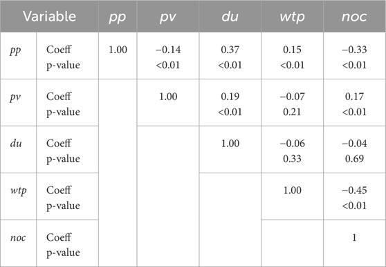
Table 3. Pearson correlation matrix.

The correlation between $pp$ and $wtp$ at 0.15 (p < 0.001) suggests that higher-weighted projects, such as residential ones, tend to progress more efficiently due to simpler workflows. In contrast, $pp$ negatively correlates with the $noc$ at −0.33, indicating that projects with more contractors are generally more complex and slower. This is supported by the positive correlation between $noc$ and $pv$ at 0.17, as larger projects often require more contractors. Additionally, $pv$ and $du$ show a small positive correlation (0.19), and $wtp$ and $noc$ are negatively correlated (−0.45), reflecting fewer contractors in higher-weighted project types. It is essential to note that some correlation values are small, even though relationships are meaningful. Small correlations can still achieve statistical significance in large sample sizes because the sample size influences the p-value. As the sample size increases, the variability in the data decreases, making even weak correlation coefficients statistically significant.

4.2.1 Conditional correlation

Table 4 presents conditional correlations between pp and $du$ across different $pv$ ranges, offering deeper insight beyond simple correlations. Projects with a $pv$ below $1 million show a moderate correlation $\left(r=0.41\right)$ between $du$ and $pp$. The strongest correlation (0.57) is found in the $1M–$5M range, indicating strong time-progress dependency. As project value increases, this correlation weakens: $5M–$15M shows a correlation of 0.49, $15M–$25M drops to 0.35, and $25M–$50M shows a correlation of 0.33, suggesting that progress becomes less time-dependent, possibly due to better resource planning or management. For projects exceeding $50M, the correlation increases slightly to 0.44, likely to reflect the complexity of large-scale projects. These findings highlight that the relationship between time and progress varies with project value, reinforcing the need to account for value-based timeframes in modelling project performance.

Table 4

Table 4. Conditional correlation.

4.3 Model framework

4.3.1 Candidate models

The results of the model comparison, using the project $du$ and $pv$ as independent variables, are shown in Table 5. Among all models tested, $MLR$ achieved the highest predictive accuracy (0.89) and the strongest agreement ($Kappa=0.72$). Gradient Boosted Machines ($GBM$) demonstrated competitive accuracy (0.84) but substantially lower agreement ($Kappa=0.27$), while Random Forest and Decision Trees exhibited weaker overall performance. These results confirm that $MLR$ outperformed $ML$ alternatives. While future research may explore tuned ML approaches, this study prioritised establishing a rigorous and transparent baseline that balances predictive performance with interpretability.

Table 5

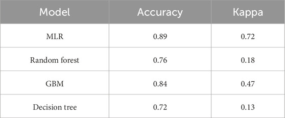
Table 5. Comparing candidate model performance.

4.3.2 Stepwise model development and selection

In this step, six MLR models were compared, with pp as the response variable and $pv$, $wtp$, $noc$, and $du$ as predictors (Table 6). The comparison indicates that $Model3$, which includes $pv$ and $du$, outperformed all others, achieving the highest Accuracy (0.89), lowest $\mathit{Log}-Loss$ (0.26), the highest Kappa (0.72), and the lowest Residual Deviance (212,220.3) and AIC (212,251.3), indicating excellent predictive power and fit. $Models1$ and $2$, which used $pv$ and $du$ separately, showed weaker performance (Accuracy: 0.75 and 0.78; Kappa: 0.31 and 0.40). Model 4, incorporating an interaction term ($pv\times du$), slightly improved Accuracy (0.86) but increased model complexity without surpassing $Model3$. $Models5$ and $6$, which added noc and wtp, achieved moderate Accuracy (0.80 and 0.79) and Kappa (0.56 and 0.55) but exhibited higher Log-Loss and AIC values, indicating reduced efficiency compared with $Model3$.

Table 6

Table 6. Model comparison results.

4.3.3 Optimal model and predictive formula

Table 7 shows that the intercepts and regression coefficients of Model three for predicting project progress at six levels (15%–100%) versus 5% are statistically significant (p < 0.05). All intercepts ($p<0.001$) reflect baseline progress probabilities. $du$ shows consistently positive, significant effects (p < 0.001), highlighting its key role in driving project advancement.

Table 7

Table 7. Model summary and coefficients for model 3.

For early progress stages like 15%, the coefficient for $pv$ is small and only marginally significant ($p=0.041$), indicating a weak relationship. As progress levels increase (30%–100%), $pv$ coefficients become increasingly negative and highly significant (p < 0.001), suggesting that higher-value projects may face delays or added complexity. In contrast, $du$ shows a strong and growing positive effect in later stages, with coefficients of 2.75 at 90% and 3.17 at 100%, confirming its critical role in achieving completion. The pronounced negative coefficient for project value at 100% $\left(-5.85e-07\right.$) further highlights challenges in managing high-value projects. These results emphasise the dominant influence of time in reaching full completion and the growing complexity linked to larger budgets. The detailed relationships between project progress and predictors (duration and value) are captured in the logit models presented in Equations 14–26.

$\mathit{L}\mathit{o}\mathit{g}\mathit{i}\mathit{t}\left(\mathit{P}5\%,15\%\right)=\mathit{ln}\left(\frac{\widehat{\mathit{P}}\left(\mathit{p}\mathit{p}=5\%\right)}{\widehat{\mathit{P}}\left(\mathit{p}\mathit{p}=15\%\right)}\right)=2.36+0.94*\mathit{d}\mathit{u}+8.10\mathit{e}-11*\mathit{p}\mathit{v}(14)$

$\mathit{L}\mathit{o}\mathit{g}\mathit{i}\mathit{t}\left(\mathit{P}5\%,30\%\right)=\mathit{ln}\left(\frac{\widehat{\mathit{P}}\left(\mathit{p}\mathit{p}=30\%\right)}{\widehat{\mathit{P}}\left(\mathit{p}\mathit{p}=5\%\right)}\right)=2.24+1.29*\mathit{d}\mathit{u}-9.70\mathit{e}-10*\mathit{p}\mathit{v}(15)$

$\mathit{L}\mathit{o}\mathit{g}\mathit{i}\mathit{t}\left(\mathit{P}5\%,50\%\right)=\mathit{ln}\left(\frac{\widehat{\mathit{P}}\left(\mathit{p}\mathit{p}=50\%\right)}{\widehat{\mathit{P}}\left(\mathit{p}\mathit{p}=5\%\right)}\right)=3.97+3.46*\mathit{d}\mathit{u}-9.10\mathit{e}-08*\mathit{p}\mathit{v}(16)$

$\mathit{L}\mathit{o}\mathit{g}\mathit{i}\mathit{t}\left(\mathit{P}5\%,70\%\right)=\mathit{ln}\left(\frac{\widehat{\mathit{P}}\left(\mathit{p}\mathit{p}=70\%\right)}{\widehat{\mathit{P}}\left(\mathit{p}\mathit{p}=5\%\right)}\right)=3.89+1.48*\mathit{d}\mathit{u}-3.30\mathit{e}-07*\mathit{p}\mathit{v}(17)$

$\mathit{L}\mathit{o}\mathit{g}\mathit{i}\mathit{t}\left(\mathit{P}5\%,90\%\right)=\mathit{ln}\left(\frac{\widehat{\mathit{P}}\left(\mathit{p}\mathit{p}=90\%\right)}{\widehat{\mathit{P}}\left(\mathit{p}\mathit{p}=5\%\right)}\right)=5.84+2.75*\mathit{d}\mathit{u}-4.11\mathit{e}-07*\mathit{p}\mathit{v}(18)$

$\mathit{L}\mathit{o}\mathit{g}\mathit{i}\mathit{t}\left(\mathit{P}5\%,100\%\right)=\mathit{ln}\left(\frac{\widehat{\mathit{P}}\left(\mathit{p}\mathit{p}=100\%\right)}{\widehat{\mathit{P}}\left(\mathit{p}\mathit{p}=5\%\right)}\right)=3.47+3.17*\mathit{d}\mathit{u}-5.85\mathit{e}-07*\mathit{p}\mathit{v}(19)$

According to Formulas $12to18$, it is possible to predict the probability of project progress based on project value at different times after the project’s commencement.

Let: $M=\exp \left(logit\left(P_{5\%,15\%}\right)\right)+\exp \left(logit\left(P_{5\%,30\%}\right)\right)+\exp$$\left(logit\left(P_{5\%,50\%}\right)\right)$ $+\mathit{exp}\left(logit\left(P_{5\%,70\%}\right)\right)+\mathit{exp}\left(logit\left(P_{5\%,90\%}\right)\right)+\mathit{exp}$$\left(logit\left(P_{5\%,100\%}\right)\right)$

Then

$\widehat{P}\left(pp=15\%\right)=\frac{\mathit{exp}\left(logit\left(P_{5\%,15\%}\right)\right)}{1+M}(20)$

$\widehat{P}\left(pp=30\%\right)=\frac{\mathit{exp}\left(logit\left(P_{5\%,30\%}\right)\right)}{1+M}(21)$

$\widehat{P}\left(pp=50\%\right)=\frac{\mathit{exp}\left(logit\left(P_{5\%,50\%}\right)\right)}{1+M}(22)$

$\widehat{P}\left(pp=70\%\right)=\frac{\exp \left(\mathit{log}\text{it}\left({\mathrm{P}}_{5\%,70\%}\right)\right)}{1+\mathrm{M}}(23)$

$\widehat{P}\left(pp=90\%\right)=\frac{\exp \left(\mathit{log}\text{it}\left({\mathrm{P}}_{5\%,90\%}\right)\right)}{1+\mathrm{M}}(24)$

$\widehat{P}\left(pp=100\%\right)=\frac{\exp \left(\mathit{log}\text{it}\left({\mathrm{P}}_{5\%,100\%}\right)\right)}{1+\mathrm{M}}(25)$

$\widehat{P}\left(pp=5\%\right)=\frac{1}{1+M}(26)$

Figure 2 illustrates the interaction between project value and duration in shaping progress stage predictions under $Model3$. The background regions represent the most likely predicted stages ($pp\sim 30\%,50\%\&100\%$), while the overlaid points denote observed projects across progress stages ($pp\sim 5\%-90\%$). The plot shows that low-value, short-duration projects are consistently predicted in earlier stages ($pp\sim 30\%$), whereas higher-value, longer-duration projects tend to be classified in later stages $\left(pp\sim 50\%-100\%\right.$). This alignment indicates that Model three effectively captures stage-based progress dynamics, with observed projects clustering closely around predicted regions. The results highlight the ability of the $Model3$ to generate reliable forecasts and provide reference ranges for expected completion times. However, greater dispersion is evident in high-value projects ($above100MNZD$), reflecting increased variability and uncertainty. Overall, the figure demonstrates how project value and duration jointly influence construction progress classification, supporting the regression outcomes.

Figure 2

Figure 2. Interaction of project value and duration in progress stage predictions (model 3).

4.3.4 Optimal model performance in class-level diagnostic

To assess the classification model’s performance, key metrics such as Odds Ratio (OR), Sensitivity, Specificity, Positive Predictive Value (PPV), Negative Predictive Value (NPV), and Balanced Accuracy (BA) were employed to evaluate predictive accuracy, error balance, and overall reliability. As presented in Table 8, the model—comprising duration and project value as predictors—illustrates how these variables influence the probability of reaching distinct project stages. The intercepts, representing baseline odds, vary across progress levels, reaching their highest value at 90% (126.24), which indicates a strong inherent likelihood of nearing completion.

Table 8

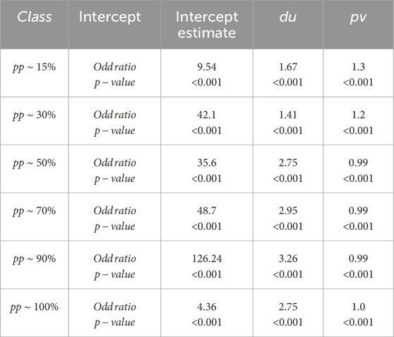
Table 8. Odds ratios for predictors for best Model.

Duration consistently exhibits a strong positive effect, with odds ratios greater than one across all stages—peaking at 90% (3.26), followed by 70% (2.95) and 50% (2.75)—underscoring its critical role in driving progress. In contrast, project value shows a modest positive impact in early stages (15%: 1.30; 30%: 1.20) but becomes less influential in later stages, with odds ratios approaching 1.00. These results suggest that while project value facilitates early-stage progress, duration remains the dominant predictor in advancing toward completion. All coefficients are statistically significant ($p<0.001$), confirming the model’s robustness. Overall, the findings affirm that time is the most critical determinant of construction progress, whereas the influence of project value diminishes as projects mature.

Table 9 summarises the model’s performance across project progress levels using key classification metrics: $Sensitivity$, $Specificity$, $PPV$, $NPV$, and $BalancedAccuracy\left(BA\right)$. $Sensitivity$ is initially low—18% at ∼5% and 28% at ∼15%—indicating limited early-stage detection but rises sharply to 81.78% at ∼30% and peaks at 89% at ∼90%, before declining slightly to 67.7% at full completion (∼100%). This pattern reflects improved accuracy in identifying projects nearing completion. $Specificity$ and $NPV$ remain consistently high, $PPV$ increases moderately, and $BA$ shows steady improvement across progress levels.

Table 9

Table 9. Confusion matrix derived metrics across project progress levels.

In contrast, $Specificity$ remains consistently high across all progress levels, starting at 99.9% (∼5%), gradually decreasing to 92.3% (∼90%), and rising again to 97.85% at 100%. This consistency suggests the model is highly reliable in identifying projects that have not yet progressed. $PPV,$ reflecting the likelihood that a predicted completed project is truly complete, the estimates start low at ∼5% (17.8%) and 15% (31.2%). It improves to 64.8% at ∼30%, peaks at 88.34% at ∼90%, but drops slightly to 64.28% at 100%, possibly due to end-stage complexities or variability. $NPV$ remains strong throughout, from 99.5% at ∼5%–96.8% at 100%, indicating high reliability in identifying incomplete projects. The average of sensitivity and specificity $\left(BA\right)$ shows steady improvement: from 58.9% at ∼5%–89.8% at ∼30%, peaking at 90.66% at ∼90%, and settling at 83.7% at 100%. This progression reflects the model’s increasing effectiveness over the project lifecycle. Overall, the model performs exceptionally well in later stages, reinforcing its utility for monitoring project progression as more data accumulates over time.

4.4 Model validation

To assess the temporal robustness of Model 3, projects commencing before 2019 were used for model training and cross-validation, while those starting from 2020 onward served as an independent temporal hold-out set for external testing. This temporal split simulated real-world forecasting conditions, where the model trained on historical data is applied to future projects. Within the training subset, a 5-fold $Cross-validation\left(CV\right)$ procedure was employed to tune the decay parameter (0, 0.01, 0.10), which controls model regularisation. The objective was to balance model complexity and generalisation capability. The CV results (Table 10) show that the model with $decay=0$ achieved the highest Accuracy (0.988) and Kappa (0.870), confirming that additional regularisation did not improve generalisation and that the unpenalised specification provided the most stable fit. The five-fold $CV$ outcomes were highly consistent across folds, with negligible variation in Accuracy (0.988 ± 0.001) and Kappa (0.870 ± 0.002), indicating that Model three was not sensitive to sampling variation and exhibited no evidence of overfitting during training.

Table 10

Table 10. Cross-validation results.

For external validation on future data (Test 2020–2022), the model’s generalisation performance was subsequently evaluated using the post-2019 dataset (Table 11). $Accuracy$ declined slightly to 0.768, with $Cohen’sKappa=0.673$, indicating substantial agreement between predicted and observed progress classes. Although this represents a small reduction from the training phase, the model maintained strong predictive capability and stable performance when applied to unseen, temporally distinct data. The minor decline likely reflects changes in project characteristics and external conditions after 2019, such as market fluctuations, regulatory updates, and pandemic-related disruptions. Nevertheless, the consistent overall performance demonstrates the model’s robustness, adaptability, and practical utility for forecasting project progress across varying temporal and economic contexts.

Table 11

Table 11. External validation results (test 2020–2022).

Table 12 presents the class-level performance metrics for Model three during the test phase. The model achieved near-perfect results for late-stage projects, with pp ∼90% and pp ∼ 70% showing almost complete sensitivity (0.999–0.986), specificity (0.996–0.999), and balanced accuracy (0.991–0.999). These results indicate that the model effectively captured the dominant patterns associated with projects nearing completion, where progress characteristics are more consistent and predictable. 1n contrast, early-stage categories (pp ∼ 5% and pp ∼ 15%) recorded low sensitivities (0.22–0.25) but very high specificities (∼0.999), leading to moderate balanced accuracies (0.61–0.62). This suggests that the model tended to underestimate early progress classes due to their higher variability and limited representation. Mid-range stages (pp ∼ 30% and pp ∼ 50%) showed mixed performance, reflecting overlapping project characteristics and transitional complexity. Overall, Model three demonstrated exceptional discriminative ability for identifying well-defined late-stage progress patterns while maintaining reasonable generalisation across all progress categories.

Table 12

Table 12. Confusion matrix derived metrics on test data.

Receiver Operating Characteristic (ROC) analysis is presented in Figure 3 and Table 13 summarises the one-vs-all ROC curves for Model three across six progress stages during the test phase. The curves show outstanding discriminative performance for pp ∼ 90% and pp ∼ 70%, which closely approach the upper-left corner of the plot, confirming near-perfect classification ability (AUC ∼0.99). Early stages such as pp ∼ 5% and pp ∼ 15% also achieved high AUC values (>0.95) despite their smaller sample sizes. In contrast, mid-stage classes (pp ∼ 30% and pp ∼ 50%) display lower curvature and greater deviation from the ideal line, indicating moderate separation due to overlapping project features. These findings highlight that the model is highly effective at identifying projects in the very early and very late stages, while predictive accuracy diminishes for intermediate progress stages where overlap in project value and duration is greatest.

Figure 3

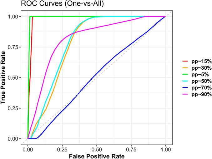
Figure 3. Receiver operating characteristic (ROC) curve for model 3.

Table 13

Table 13. Area under the ROC curve (AUC) for each progress stage (model 3).

Table 14 presents the year-by-year performance of Model three across the test period. Accuracy remained strong in 2020 (0.865) and 2021 (0.894) but dropped sharply to 0.520 in 2022, revealing a clear temporal drift in predictive stability. This deterioration suggests that post-pandemic shifts in construction cost structures, labour availability, and project management practices altered the relationships learned from pre-2019 data. Broader external disruptions, including supply chain delays, material price escalations, and regulatory changes, further reshaped progress dynamics. These findings underscore the need for continuous recalibration and adaptive model updating to sustain forecasting accuracy amid evolving economic and industry conditions.

Table 14

Table 14. Year-by-year Model performance (test 2020–2022).

Taken together, the results from the cross-validation, external validation, confusion matrix, and $ROC$ analyses confirm the model’s strong and coherent performance across multiple evaluation dimensions. The five-fold cross-validation (Table 10) demonstrated excellent internal stability ($Accuracy=0.988;Kappa=0.870$) with no signs of overfitting, while external validation on post-2019 data (Table 11) showed only a modest decline ($Accuracy=0.768;Kappa=0.673$), indicating good temporal generalisation. Class-level metrics (Table 12) further revealed that the model captured late-stage progress patterns with near-perfect sensitivity and specificity, while moderate accuracy for early stages reflected class imbalance and variability. Consistently, the ROC analysis (Figure 3; Table 13) reported high $AUC$ values for both early and late stages (>0.95), confirming strong separability across thresholds. Together, these findings demonstrate that Model three performs reliably, generalises well over time, and maintains excellent discriminative capability across progress categories.

4.5 Practical implications in real-world scenarios

Using the optimal model, Equations 20–26 estimate project progress at different stages based on project size, incorporating key predictors like value and duration. The model is applied to real-world data from New Zealand’s construction sector to predict progress milestones and support better planning and resource allocation. As shown in Figure 4, predicted progress varies across durations from one to 6 years ($du=1to6$), depending on $pv$. The analysis reveals that smaller projects tend to reach milestones faster, while larger projects face greater challenges due to increased complexity. These findings emphasise the importance of accounting for both size and duration when forecasting construction progress, enabling more effective project management and reducing the risk of delays or budget overruns.

Figure 4

Figure 4. Probability of project progress for various project values (NZD) and durations (du). (a) Probability of project progress after one year (du = 1). (b) Probability of project progress after two years (du = 2). (c) Probability of project progress after three years (du = 3). (d) Probability of project progress after four years (du = 4). (e) Probability of project progress after five years (du = 5). (f) Probability of project progress after six years (du = 6).

According to Figures 4a, after 1 year ($du=1$), smaller projects, such as those valued at $500k$, exhibit a high probability of achieving full completion ($pp=100\%$), approximately 0.91. This highlights their efficiency in meeting objectives quickly due to their simpler scope and reduced complexity. In contrast, moderate projects valued at $15M have a significantly lower probability of full completion within 1 year, around 0.02. However, their probability of reaching an intermediate progress level (pp = 50%) is 0.27, indicating steady, albeit slower, advancement. By the second year (du = 2), the probability for these moderate projects to achieve pp = 50% increases to 0.43, showcasing sustained progress over time.

$P\left(\left.pp=100\%\right|pv=500k,du=1\right)\simeq 0.91$

$P\left(\left.pp=100\%\right|pv=15M,du=1\right)\simeq 0.02$

$P\left(\left.pp=50\%\right|pv=15M,du=1\right)\simeq 0.27$

By the second year, according to Figures 4b, moderate projects display increasing probabilities of intermediate progress levels (e.g., pp = 30%, pp = 50%). In contrast, smaller projects show signs of stagnation due to potential resource constraints or unforeseen challenges. For larger projects valued at $50M, the probability of achieving early progress (pp = 15%) after 2 years is 0.34, while moderate progress (pp = 30%) reaches 0.59. This indicates that larger projects face greater initial challenges but gradually overcome them.

$P\left(\left.pp=15\%\right|pv=50M,du=2\right)\simeq 0.34$,

$P\left(\left.pp=30\%\right|pv=50M,du=2\right)\simeq 0.59$

At 3 years, according to Figures 4c, moderate projects emerge as the most consistent performers, with a significant increase in the probability of achieving moderate stages. For instance, the probability of moderate progress (pp = 30%) for $50M projects improves slightly to 0.61, while for $50M projects, pp = 50% reaches 0.08. This demonstrates steady, albeit slower, advancement for these projects. In contrast, larger projects continue to face challenges that impede rapid progress due to their complexity and scope.

$P\left(\left.pp=30\%\right|pv=50M,du=3\right)\simeq 0.61$,

$P\left(\left.pp=50\%\right|pv=50M,du=3\right)\simeq 0.08$

By the fourth year, as shown in Figures 4d, moderate projects stabilise in their progress probabilities, achieving high levels of completion. For instance, the probability of achieving pp = 70% for $30M projects is 0.53, while for $50M projects, it is 0.48. Similarly, the probability of pp = 50% for $30M projects stabilises around 0.47. Small projects also begin to reach a higher probability of completion, provided their challenges are resolved. However, large projects remain delayed, as their extensive scope and dependencies create barriers to timely completion.

$P\left(\left.pp=70\%\right|pv=30M,du=4\right)\simeq 0.53$

$P\left(\left.pp=50\%\right|pv=30M,du=4\right)\simeq 0.43$

$P\left(\left.pp=70\%\right|pv=50M,du=4\right)\simeq 0.48$

$P\left(\left.pp=50\%\right|pv=30M,du=4\right)\simeq 0.47$

In the fifth and sixth years, as shown in Figures 4e,f, moderate projects consistently achieve near completion or full completion, reflecting their optimal balance between value and complexity. For example, the probability of achieving $pp=70\%$ with a value $ of $100M is 0.43 by the fifth year, increasing to 0.65 by the sixth year. These results highlight the gradual improvement of large projects, although their progress remains slower due to inherent challenges such as resource mismanagement and external dependencies.

$P\left(\left.pp=70\%\right|pv=100M,du=5\right)\simeq 0.43$

$P\left(\left.pp=70\%\right|pv=100M,du=6\right)\simeq 0.65$

Overall, smaller projects demonstrate faster progress and higher completion probabilities within shorter durations, while moderate projects achieve steady and balanced advancement over time. Larger projects require extended durations to overcome complexities, with their progress becoming more significant only in later years. These findings underscore the importance of tailoring project management strategies to account for project value and duration to optimise outcomes and address challenges effectively.

The results also support monitoring and risk detection. For instance, if a project of a given size is expected to reach 50% completion after 2 years but actual progress falls short, this signals a potential issue. Project managers can then combine insights from the model with on-site observations and stakeholder feedback to diagnose the cause and decide whether to reallocate resources, renegotiate milestones, or introduce contingency measures.

5 Discussion

This study identifies project size, project type, duration, and the number of contractors as key determinants of construction progress. Among these, project size and duration emerged as the most critical predictors, forming the foundation for accurate forecasting and effective planning—both of which are essential for project success. Incorporating conditional correlation analysis enhanced the model’s robustness by revealing how these factors interact to influence project performance.

These findings align with previous research, which consistently links inadequate planning to project delays and cost overruns (Assaad et al., 2020; Kerzner, 2022; Shah, 2016). Prior studies have also underscored the significance of project characteristics: Cao et al. (2015) highlighted the combined effects of project size and type on performance; Chao and Chen (2015) examined duration and contractor count; and Picornell et al. (2017) and Alaloul et al. (2016) confirmed the influence of contractor numbers. More recent investigations by Santolini et al. (2021), Sekar et al. (2021), Azmat and Siddiqui (2023), and Ackon et al. (2025) further validated the role of project size and contractor-related factors in determining project outcomes. While these studies offer valuable insights, they often analyse these variables in isolation or through qualitative assessments. In contrast, the present study integrates them into a unified quantitative model, providing a more holistic understanding of their combined effects on project performance. Moreover, whereas previous research typically assessed project success as a single outcome, this study examines progress across distinct project stages—addressing a key gap by offering stage-based insights into construction performance.

Building on this foundation, the multinomial logistic regression (MLR) model was selected as the primary analytical approach due to its interpretability, statistical rigor, and suitability for handling multiple outcome categories. To benchmark its performance and ensure robustness, several alternative ML algorithms—including Random Forest, Gradient Boosting, and Decision Trees—were evaluated. The results confirmed that MLR outperformed these ML alternatives, demonstrating stronger predictive consistency and interpretability. Subsequently, six MLR models were developed and compared to evaluate how project duration, project value, project type, and the number of contractors jointly influence construction progress. Variables were introduced sequentially, starting with project value and duration, followed by their interaction term, and subsequently by project type and contractor count. This stepwise procedure enabled the identification of both individual and interactive effects of predictors, aligning with the methodological recommendations of Proaño-Narváez et al. (2022), who emphasised the importance of diverse modelling strategies to enhance predictive accuracy and interpretability. Among the six specifications, the model incorporating project duration and project value (Model 3) demonstrated the best overall fit and predictive performance (Accuracy = 0.89; Kappa = 0.72), confirming the dominant role of these two variables in explaining construction progress dynamics.

The model’s performance was rigorously evaluated using odds ratios and confusion matrix–derived metrics to assess its accuracy and reliability. The odds ratio analysis revealed a strong positive association between project duration and progress, particularly at later stages of completion, where longer durations substantially increased the likelihood of achieving full completion. In contrast, project value showed a modest positive impact in early stages but became less influential as projects advanced, reflecting the growing complexity, coordination, and resource intensity of larger projects. These results suggest that while project value facilitates early-stage advancement, duration remains the dominant predictor driving projects toward completion.

The classification-based evaluation further confirmed the model’s robustness across progress levels. High sensitivity and PPV were observed at advanced stages, while consistently high NPV indicated reliable identification of incomplete projects. The model performed exceptionally well in later stages, reinforcing its utility for monitoring project progression as more data accumulates over time. Collectively, these findings demonstrate that the model effectively distinguishes between incomplete and near-complete projects, aligning with observed decision boundaries where smaller projects tend to advance more rapidly and larger ones stabilise at mid-to-late stages.

Cross-validation reinforced these findings, yielding high overall accuracy and Kappa values. The five-fold cross-validation demonstrated excellent internal stability (Accuracy = 0.988; Kappa = 0.870) with no indication of overfitting, confirming robustness under varied data partitions. External validation on post-2019 data showed only a modest decline in performance (Accuracy = 0.768; Kappa = 0.673), indicating strong temporal generalisability and resilience to distributional shifts. Class-level assessment revealed near-perfect sensitivity and specificity at late stages of completion, while moderate accuracy at early stages reflected expected class imbalance and variability in progress patterns. Real-world evidence supports these results: smaller projects progress faster due to reduced complexity (Assaad et al., 2020; Jaber et al., 2020), whereas larger projects valued at approximately $15M face early-stage challenges but advance steadily at intermediate stages, further reinforcing duration as a critical predictor. Consistently, ROC analysis reported AUC values above 0.95 across early and late stages, confirming excellent separability and coherence across progress categories. Overall, these results demonstrate that Model three performs reliably, generalises effectively across time horizons, and maintains strong discriminative capability in predicting construction progress at different stages.

When compared with recent ML developments, the proposed MLR model shows competitive performance while maintaining interpretability. Previous ML studies, such as those by Guo et al. (2019); Jaber et al. (2020) achieved R² values between 0.66 and 0.80, while Egwim et al. (2021) reported 76% accuracy using ensemble methods. Although advanced frameworks such as LightGBM, CatBoost, and GAN architecture have reached accuracies above 90% (Alsulamy, 2025),these models often operate as opaque “black boxes” with high computational demands. In contrast, the MLR model bridges the gap between traditional and AI-based approaches by combining statistical transparency with strong predictive power. It achieved superior accuracy and agreement compared with ML methods such as Random Forest, Gradient Boosting, and Decision Trees. Unlike complex ML models that capture non-linearities but lack explainability (Akinosho et al., 2020; Regona et al., 2022a; Regona et al., 2022b), MLR offers theoretical grounding and practical applicability, enabling confident, insight-driven decision-making across academic and industry contexts.

The model’s ability to predict progress at specific milestones positions it as a strong foundation for data-driven construction management and an early step toward adaptive systems—such as digital twins—that enable dynamic monitoring and informed decision-making. Compared with traditional methods such as S-curve modelling (Chao and Chen, 2015) and BIM-based approaches (Cao et al., 2015), which primarily assesses overall project completion, the proposed model forecasts progress at distinct stages, offering greater adaptability to evolving project conditions. With an overall accuracy of 89%, it outperforms Earned Value–based approaches (Ballesteros-Pérez et al., 2020a; Colin and Vanhoucke, 2015; Nizam and Elshannaway, 2019; Proaño-Narváez et al., 2022) and demonstrates higher reliability than advanced EVM extensions such as EVM-SNB (80% accuracy) and EVM-FPB (83% efficiency) reported by Colin and Vanhoucke (2015). These findings underscore the practical value of stage-specific forecasting in enhancing real-time control and supporting adaptive management strategies within complex construction environments.

In summary, this study demonstrates that interpretable statistical models can deliver high predictive accuracy while maintaining transparency and practical relevance. The multinomial logistic regression (MLR) framework effectively forecasts construction progress at distinct milestones, bridging the gap between traditional and AI-based approaches. Its strong performance highlights the potential of explainable analytics to enhance early warning, adaptive control, and data-driven decision-making in construction management. By combining statistical rigor with interpretability, the model provides a scalable foundation for integrating predictive insights into emerging digital systems such as digital twins, supporting more intelligent and resilient project delivery.

6 Limitations

While the proposed model offers strong predictive accuracy, it has limitations. It performs best for projects without major unforeseen challenges, as its assumptions align better with consistent data patterns. A key limitation is its reliance on historical data, which may not capture unprecedented events such as policy shifts or technological advances. Although expert-reviewed and preprocessed, the model also relies on the accurate reporting of variables such as project value and contractor involvement—any inconsistencies can impact its reliability. Additionally, it does not fully account for non-linear relationships or complex external factors, such as workforce issues or supply chain disruptions, which limits its accuracy in highly uncertain scenarios. Finally, because the training data is specific to New Zealand, the generalisability of the findings to international contexts remains limited without appropriate recalibration. In this regard, challenges remain in extending the framework to international datasets where regulatory, cultural, and economic factors differ significantly.

Despite these constraints, the model represents a significant advancement in forecasting construction progress. Incorporating project value, duration, and contractor variables into a multinomial logistic regression framework, it offers an interpretable, accurate, and stage-based tool for project monitoring. This approach supports early risk identification, better resource allocation, and improved decision-making. It also contributes to sustainable construction by reducing delays and rework. Future research could address current gaps by (i) validating the framework across international datasets, (ii) incorporating additional variables that capture macroeconomic and environmental uncertainty, and (iii) comparing the multinomial logistic regression approach with more advanced machine learning and hybrid AI methods. Such developments would further enhance adaptability, scalability, and robustness, ensuring the model remains relevant for both local and global applications. Ultimately, this framework aligns with Industry 5.0 principles through its human-centric, data-driven methodology, where AI enhances rather than replaces strategic oversight.

7 Contributions and implications

This study introduces a robust statistical model that enables probabilistic predictions of project progress by integrating key variables—time and project value—into a unified framework. Unlike prior studies that examine these factors independently, this model provides a comprehensive and quantifiable perspective on the dynamics influencing construction performance. Its stage-based structure allows for progress estimation at critical milestones (e.g., 5%, 15%, 30%), addressing a key gap in existing research that predominantly focuses on overall project completion as a single outcome. Developed using multinomial logistic regression, the model ensures transparency and interpretability, offering a practical alternative to complex “black-box” machine-learning techniques and traditional methods such as S-curve analysis, Earned Value Management (EVM), and Risk Management (RM).

Beyond methodological advancement, the model offers tangible practical value. It can be integrated into digital dashboards to generate real-time progress probabilities and performance alerts, enabling project managers to anticipate delays, optimise resource use, and improve planning accuracy. For client-side managers, it provides a transparent tool to evaluate contractor performance against milestones, while at the portfolio level, aggregated outputs can help policymakers and regulators monitor sector-wide progress, assess workload pressures, and inform decisions on resource allocation, cost escalation, and workforce planning. This framework promotes collaboration, sustainability, and resilience within the construction sector, offering both a novel analytical tool and a strategic foundation for advancing predictive, transparent, and adaptive project management practices.

8 Conclusion

This paper presents a predictive model for the construction industry, grounded in statistical theory and validated with real-world data. By analysing cost, time, contractor involvement, and project type, the model identifies project duration and value as the most influential predictors of progress. While the inclusion of contractor and project-type variables produced reasonable model performance, these additions did not substantially enhance predictive accuracy. The combination of project duration and value alone achieved the strongest results, highlighting their dominant role in explaining construction progress dynamics. The model’s stage-based forecasting approach—rather than a single completion estimate—supports informed decision-making, resource optimisation, and proactive project control. Its clear equations and visual output improve interpretability and facilitate practical implementation.

Using data from New Zealand’s construction sector, the model demonstrated strong reliability and robustness, advancing understanding of how project characteristics influence progress and enabling early identification of at-risk projects to prevent delays and cost overruns. Beyond individual projects, the framework can be scaled for portfolio-level analysis, allowing organisations and policymakers to monitor multiple projects, assess workload distribution, and identify systemic risks. Its adaptable structure also allows for application across various sectors, including manufacturing, transportation, and energy. Future research could integrate this framework with digital dashboards or AI-driven systems to enhance real-time monitoring and forecasting. Broader adoption of this model can improve project and portfolio outcomes, strengthen data-driven management practices, and contribute to more efficient and resilient delivery systems.

Data availability statement

The data analyzed in this study is subject to the following licenses/restrictions: The data sets used in this study are not publicly available due to institutional restrictions but are available from the corresponding author upon reasonable request. Requests to access these datasets should be directed to Requests to access the dataset may be directed to: Maryam Tagharobi Corresponding Author School of Built Environment, Massey University, New Zealand bS50YWdoYXJvYmlAbWFzc2V5LmFjLm56 Please note that the dataset is part of the Can-Construct Project, funded by the New Zealand Ministry of Business, Innovation and Employment (MBIE). Due to confidentiality agreements and the expenses involved in data preparation, access is restricted and may require formal approval and a data-sharing agreement.

Author contributions

MT: Conceptualization, Data curation, Formal analysis, Investigation, Methodology, Project administration, Resources, Software, Validation, Visualization, Writing – original draft, Writing – review and editing. MB: Supervision, Funding acquisition, Writing – review and editing. TS: Supervision, Writing – review and editing.

Funding

The authors declare that financial support was received for the research and/or publication of this article. This work was supported by the New Zealand Ministry of Business, Innovation and Employment (MBIE) under Grant MAUX2005.

Acknowledgements

The authors acknowledge the support provided through the Endeavour Programmed Research Grant titled “Creating Capacity and Capability for New Zealand Construction.”

Conflict of interest

The authors declare that the research was conducted in the absence of any commercial or financial relationships that could be construed as a potential conflict of interest.

Generative AI statement

The authors declare that no Generative AI was used in the creation of this manuscript.

Any alternative text (alt text) provided alongside figures in this article has been generated by Frontiers with the support of artificial intelligence and reasonable efforts have been made to ensure accuracy, including review by the authors wherever possible. If you identify any issues, please contact us.

Publisher’s note

All claims expressed in this article are solely those of the authors and do not necessarily represent those of their affiliated organizations, or those of the publisher, the editors and the reviewers. Any product that may be evaluated in this article, or claim that may be made by its manufacturer, is not guaranteed or endorsed by the publisher.

References

Abdallah, A. A., Shaawat, M. E., and Almohassen, A. S. (2024). Causes of miscommunication leading to project delays and low work quality in the construction industry of Saudi Arabia. Ain Shams Eng. J. 15 (3), 102447. doi:10.1016/j.asej.2023.102447

CrossRef Full Text | Google Scholar

Ackon, F., Mensah, J., Danso, H., and Nyarko, I. (2025). Influence of contractors’ management strategies on construction project performance in developing economies. Afr. J. Appl. Res. 11 (1), 51–68. doi:10.26437/ajar.v11i1.825

CrossRef Full Text | Google Scholar

Adamtey, S., and Kereri, J. O. (2023). Risk management in residential projects in the United States: implementation status, evaluation techniques and barriers. J. Eng. Des. Technol. 21 (5), 1481–1500. doi:10.1108/jedt-05-2021-0246

CrossRef Full Text | Google Scholar

Ahmadzai, M. B., and Ye, K. (2025). A mixed-method investigation of the root causes of construction project delays in Afghanistan. Heliyon 11 (2), e41923. doi:10.1016/j.heliyon.2025.e41923

PubMed Abstract | CrossRef Full Text | Google Scholar

Akinosho, T. D., Oyedele, L. O., Bilal, M., Ajayi, A. O., Delgado, M. D., Akinade, O. O., et al. (2020). Deep learning in the construction industry: a review of present status and future innovations. J. Build. Eng. 32, 101827. doi:10.1016/j.jobe.2020.101827

CrossRef Full Text | Google Scholar

Al-Gahtani, K. S., Alsugair, A. M., Alsanabani, N. M., Alabduljabbar, A. A., and Almutairi, B. (2022). Forecasting delay-time model for Saudi construction projects using DEMATEL–SD technique. Int. J. Constr. Manag. 24, 1225–1239. doi:10.1080/15623599.2022.2152944

CrossRef Full Text | Google Scholar

Al-Ghzawi, M., and El-Rayes, K. (2024). Machine learning and multi-objective optimization methodology for planning construction phases of airport expansion projects. J. Air Transp. Manag. 115, 102550. doi:10.1016/j.jairtraman.2024.102550

CrossRef Full Text | Google Scholar

Alaloul, W. S., Liew, M. S., and Zawawi, N. A. W. A. (2016). Identification of coordination factors affecting building projects performance. Alexandria Eng. J. 55 (3), 2689–2698. doi:10.1016/j.aej.2016.06.010

CrossRef Full Text | Google Scholar

Alboğa, Ö., Tantekin Celik, G., Ün, B., Aydınlı, S., and Erdis, E. (2025). The effects of COVID-19 on the construction sector: before and after. Int. J. Disaster Risk Reduct. doi:10.1016/j.ijdrr.2025.105278

CrossRef Full Text | Google Scholar

Alizadehsalehi, S., and Yitmen, I. (2016). The impact of field data capturing technologies on automated construction project progress monitoring. Procedia Eng. 161, 97–103. doi:10.1016/j.proeng.2016.08.504

CrossRef Full Text | Google Scholar

Alsaedi, A., and Naimi, S. (2024). A novel time management approach for the construction industry: a mathematical analysis. Math. Model. Eng. Problems 11, 210–216. doi:10.18280/mmep.110123

CrossRef Full Text | Google Scholar

Alsulamy, S. (2025). Predicting construction delay risks in Saudi Arabian projects: a comparative analysis of CatBoost, XGBoost, and LGBM. Expert Syst. Appl. 268, 126268. doi:10.1016/j.eswa.2024.126268

CrossRef Full Text | Google Scholar

Anand, H., Nateghi, R., and Alemazkoor, N. (2023). Bottom-up forecasting: applications and limitations in load forecasting using smart-meter data. Data-Centric Eng. 4, e14. doi:10.1017/dce.2023.10

CrossRef Full Text | Google Scholar

Anwar, M., Kurniyaningrum, E., Pontan, D., and Innavona, I. (2024). Evaluation of cost and time performance control using the concept method of earned value in the purwodadi market development project, argamakmur district. Sidoarjo, Indonesia: North Bengkulu Regency. Eduvest - Journal of Universal Studies.

Google Scholar

Assaad, R., El-Adaway, I. H., and Abotaleb, I. S. (2020). Predicting project performance in the construction industry. J. Constr. Eng. Manag. 146 (5), 04020030. doi:10.1061/(asce)co.1943-7862.0001797

CrossRef Full Text | Google Scholar

Azmat, Z., and Siddiqui, M. A. (2023). Analyzing project complexity, its dimensions and their impact on project success. Systems 11 (8), 417. doi:10.3390/systems11080417

CrossRef Full Text | Google Scholar

Bajomo, M., Ogbeyemi, A., and Zhang, W. (2022). A systems dynamics approach to the management of material procurement for engineering, procurement and construction industry. Int. J. Prod. Econ. 244, 108390. doi:10.1016/j.ijpe.2021.108390

CrossRef Full Text | Google Scholar

Ballesteros-Pérez, P., and Elamrousy, K. M. (2018). in On the limitations of the earned value management technique to anticipate project delays. Editors M. Abdul-Malak, H. Khoury, A. Singh, and S. Yazdani

Google Scholar

Ballesteros-Pérez, P., Cerezo-Narváez, A., Otero-Mateo, M., Pastor-Fernández, A., Zhang, J., and Vanhoucke, M. (2020a). Forecasting the project duration average and standard deviation from deterministic schedule information. Appl. Sci. 10 (2), 654. doi:10.3390/app10020654

CrossRef Full Text | Google Scholar

Ballesteros-Pérez, P., Sanz-Ablanedo, E., Soetanto, R., González-Cruz, M. C., Larsen, G. D., and Cerezo-Narváez, A. (2020b). Duration and cost variability of construction activities: an empirical study. J. Constr. Eng. Manag. 146 (1), 04019093. doi:10.1061/(asce)co.1943-7862.0001739

CrossRef Full Text | Google Scholar

Bertram, N., Fuchs, S., Mischke, J., Palter, R., Strube, G., and Woetzel, J. (2019). Modular construction: from projects to products. McKinsey and Co. Cap. Proj. and Infrastructure 1, 1–34.

Google Scholar

Boudreaux, C. J., Jha, A., and Escaleras, M. (2023). Natural disasters, entrepreneurship activity, and the moderating role of country governance. Small Bus. Econ. 60 (4), 1483–1508. doi:10.1007/s11187-022-00657-y

CrossRef Full Text | Google Scholar

Burrell, J. (2016). How the machine ‘thinks’: understanding opacity in machine learning algorithms. Big Data and Soc. 3, 2053951715622512. doi:10.1177/2053951715622512

CrossRef Full Text | Google Scholar

Cao, D., Wang, G., Li, H., Skitmore, M., Huang, T., and Zhang, W. (2015). Practices and effectiveness of building information modelling in construction projects in China. Automation Constr. 49, 113–122. doi:10.1016/j.autcon.2014.10.014

CrossRef Full Text | Google Scholar

Carvalho, D. V., Pereira, E. M., and Cardoso, J. S. (2019). Machine learning interpretability: a survey on methods and metrics. Electronics 8 (8), 832. doi:10.3390/electronics8080832

CrossRef Full Text | Google Scholar

Castañeda, K., Sánchez, O., Herrera, R. F., and Mejía, G. (2025). Deficiencies causes in road construction scheduling: perspectives from construction professionals. Heliyon 11 (2), e41514. doi:10.1016/j.heliyon.2024.e41514

PubMed Abstract | CrossRef Full Text | Google Scholar

Chao, L.-C., and Chen, H.-T. (2015). Predicting project progress via estimation of S-curve's key geometric feature values. Automation Constr. 57, 33–41. doi:10.1016/j.autcon.2015.04.015

CrossRef Full Text | Google Scholar

Colin, J., and Vanhoucke, M. (2015). A comparison of the performance of various project control methods using earned value management systems. Expert Syst. Appl. 42 (6), 3159–3175. doi:10.1016/j.eswa.2014.12.007

CrossRef Full Text | Google Scholar

Daoud, A. O., El Hefnawy, M., and Wefki, H. (2023). Investigation of critical factors affecting cost overruns and delays in Egyptian mega construction projects. Alexandria Eng. J. 83, 326–334. doi:10.1016/j.aej.2023.10.052

CrossRef Full Text | Google Scholar

Dattadean, M. M. (2016). Mathematical techniques employed in planning a construction project: case study on the construction of retaining walls. Int. J. Manag. Sci. Bus. Adm. 3, 41–47. doi:10.18775//ijmsba.1849-5664-5419.2014.31.1004

CrossRef Full Text | Google Scholar

de Sá Pedroso, M. F. (2017). Application of machine learning techniques in project management tools (Master’s thesis). Instituto Superior Técnico, Universidade de Lisboa.

Google Scholar

Ding, Z., Yi, G., Tam, V. W., and Huang, T. (2016). A system dynamics-based environmental performance simulation of construction waste reduction management in China. Waste Manag. 51, 130–141. doi:10.1016/j.wasman.2016.03.001

PubMed Abstract | CrossRef Full Text | Google Scholar

Durdyev, S., and Hosseini, M. R. (2020). Causes of delays on construction projects: a comprehensive list. Int. J. Manag. Proj. Bus. 13 (1), 20–46. doi:10.1108/ijmpb-09-2018-0178

CrossRef Full Text | Google Scholar

Egwim, C. N., Alaka, H., Toriola-Coker, L. O., Balogun, H., and Sunmola, F. (2021). Applied artificial intelligence for predicting construction projects delay. Mach. Learn. Appl. 6, 100166. doi:10.1016/j.mlwa.2021.100166

CrossRef Full Text | Google Scholar

El-Habil, A. M. (2012). An application on multinomial logistic regression model. Pak. J. statistics operation Res. 8, 271–291. doi:10.18187/pjsor.v8i2.234

CrossRef Full Text | Google Scholar

Fakunle, F. F., and Fashina, A. A. (2020). Major delays in construction projects: a global overview. PM World J. 9, 1–15.

Google Scholar

Gamil, Y., and Abdul Rahman, I. (2020). Assessment of critical factors contributing to construction failure in Yemen. Int. J. Constr. Manag. 20 (5), 429–436. doi:10.1080/15623599.2018.1484866

CrossRef Full Text | Google Scholar

Getawa Ayalew, G., and Ayalew, G. M. (2024). Developing fuzzy-based earned value analysis model for estimating the performance of construction projects. A case of selected public building projects in Ethiopia. Cogent Eng. 11, 2348210. doi:10.1080/23311916.2024.2348210

CrossRef Full Text | Google Scholar

Ghoroqi, M., Ghoddousi, P., Makui, A., Shirzadi Javid, A. A., and Talebi, S. (2023). An integrated model for multi-mode resource-constrained multi-project scheduling problems considering supply management with sustainable approach in the construction industry under uncertainty using evidence theory and optimization algorithms. Buildings 13, 2023. doi:10.3390/buildings13082023

CrossRef Full Text | Google Scholar

Guo, J. X., Hu, C. M., and Bao, R. (2019). Predicting the duration of a general contracting industrial project based on the residual modified model. KSCE J. Civ. Eng. 23(8), 3275–3284.

CrossRef Full Text | Google Scholar

Ingle, P. V., and Mahesh, G. (2024). Exploring performance areas and developing performance assessment model for a construction projects in India. J. Facil. Manag. 22 (4), 521–547. doi:10.1108/jfm-05-2022-0050

CrossRef Full Text | Google Scholar

Ingle, P. V., Mahesh, G., and Md, D. (2021). Identifying the performance areas affecting the project performance for Indian construction projects. J. Eng. Des. Technol. 19 (1), 1–20. doi:10.1108/jedt-01-2020-0027

CrossRef Full Text | Google Scholar

Ismaila, U., Jung, W., and Park, C. Y. (2022). Delay causes and types in Nigerian power construction projects. Energies 15 (3), 814. doi:10.3390/en15030814

CrossRef Full Text | Google Scholar

Jaber, F. K., Jasim, N. A., and Al-Zwainy, F. M. (2020). Forecasting techniques in construction industry: earned value indicators and performance models. Sci. Rev. Eng. Environ. Sci. (SREES) 29 (2), 234–243. doi:10.22630/pniks.2020.29.2.20

CrossRef Full Text | Google Scholar

Jiang, S., Yang, B., and Liu, B. (2025). Precast components On-site construction planning and scheduling method based on a novel deep learning integrated multi-agent system. J. Build. Eng. 102, 111907. doi:10.1016/j.jobe.2025.111907

CrossRef Full Text | Google Scholar

Johansen, K., Schultz, C., and Teizer, J. (2025). Knowledge graph exploitation to enhance the usability of risk assessment in construction safety planning. Adv. Eng. Inf. 65, 103305. doi:10.1016/j.aei.2025.103305

CrossRef Full Text | Google Scholar

Kazar, G., and Küçük, M. (2024). Project characteristic-based performance prediction model for school constructions: hierarchical regression approach. Rev. construcción 23 (2), 296–316. doi:10.7764/rdlc.23.2.296

CrossRef Full Text | Google Scholar

Keng, T. C., and Shahdan, N. (2015). The application of earned value management (Evm) in construction project management. J. Technol. Manag. Bus. 2 (2).

Google Scholar

Kerzner, H. (2022). Project management metrics, KPIs, and dashboards: a guide to measuring and monitoring project performance. Hoboken, NJ, United States: John Wiley & Sons.

Google Scholar

Kim, Y.-J., Yeom, D.-J., and Kim, Y. S. (2019). Development of construction duration prediction model for project planning phase of mixed-use buildings. J. Asian Archit. Build. Eng. 18, 586–598. doi:10.1080/13467581.2019.1696207

CrossRef Full Text | Google Scholar

Klingsad, R., and Ayudhya, B. I. N. (2025). Impact of COVID-19 on supply chain performance: a case of civil railway construction projects. Procedia Comput. Sci. 256, 1445–1450. doi:10.1016/j.procs.2025.02.277

CrossRef Full Text | Google Scholar

Koirala, M. P., and Shahi, R. S. (2024). Examining the causes and effects of time overruns in construction projects promoted by rural municipalities in Nepal. Eval. Program Plan. 105, 102436. doi:10.1016/j.evalprogplan.2024.102436

PubMed Abstract | CrossRef Full Text | Google Scholar

Kumar, R., and Mouli, T. C. (2018). Scheduling under uncertainties using fuzzy mathematical model.

Google Scholar

Lalmi, A., Boumali, B.-E., Fernandes, G., and Boudemagh, S. S. (2025). Identifying the Most used traditional project management practices in construction industry. Procedia Comput. Sci. 256, 1756–1763. doi:10.1016/j.procs.2025.02.315

CrossRef Full Text | Google Scholar

Leon, H., Osman, H., Georgy, M., and Elsaid, M. (2018). System dynamics approach for forecasting performance of construction projects. J. Manag. Eng. 34 (1), 04017049. doi:10.1061/(asce)me.1943-5479.0000575

CrossRef Full Text | Google Scholar

Liang, J., Bi, G., and Zhan, C. (2020). Multinomial and ordinal logistic regression analyses with multi-categorical variables using R. Ann. Transl. Med. 8 (16), 982. doi:10.21037/atm-2020-57

PubMed Abstract | CrossRef Full Text | Google Scholar

Liben, S. M., Belachew, D. A., and Elsaigh, W. A. (2024). Comparing advanced and traditional machine learning algorithms for construction duration prediction: a case study of addis Ababa’s public sector. Eng. Res. Express, 6. doi:10.1088/2631-8695/ad979f

CrossRef Full Text | Google Scholar

Lin, Y., Deng, X., Li, X., and Ma, E. (2014). Comparison of multinomial logistic regression and logistic regression: which is more efficient in allocating land use? Front. Earth Sci. 8, 512–523. doi:10.1007/s11707-014-0426-y

CrossRef Full Text | Google Scholar

Luce, R. D. (1959). Individual choice behavior, 4. New York: Wiley.

Google Scholar

Merdžanović, I., Vukomanović, M., and Ivandić Vidović, D. (2023). “A comprehensive literature review of research trends of applying AI to construction project management,” in Proceedings of the 6th IPMA SENET project management conference “digital transformation and sustainable development in project management.

Google Scholar

Mohammadjafari, A., Ghannadpour, S. F., Bagherpour, M., and Zandieh, F. (2024). Multi-objective multi-mode time-cost tradeoff modeling in construction projects considering productivity improvement. ArXiv, abs/2401.12388.

Google Scholar

Morozovskiy, P., Kulish, I., Muradov, D., and Kulakov, K. (2019). Statistical modeling of residential complex construction project. E3S Web Conf. 91, 08001. doi:10.1051/e3sconf/20199108001

CrossRef Full Text | Google Scholar

Nadafi, S., Moosavirad, S. H., and Ariafar, S. (2019). Predicting the project time and costs using EVM based on gray numbers. Eng. Constr. Archit. Manag. 26 (9), 2107–2119. doi:10.1108/ecam-07-2018-0291

CrossRef Full Text | Google Scholar

Ngo, K. A., Lucko, G., and Ballesteros-Pérez, P. (2022). Continuous earned value management with singularity functions for comprehensive project performance tracking and forecasting. Automation Constr. 143, 104583. doi:10.1016/j.autcon.2022.104583

CrossRef Full Text | Google Scholar

Nizam, A., and Elshannaway, A. (2019). Review of earned value management (EVM) methodology, its limitations, and applicable extensions. J. Manag. and Eng. Integration 12 (1), 59–70. doi:10.62704/10057/24251

CrossRef Full Text | Google Scholar

Olanipekun, A. O., Xia, B., Hon, C., and Darko, A. (2018). Effect of motivation and owner commitment on the delivery performance of green building projects. J. Manage. Eng. 34 (1), 04017039.

CrossRef Full Text | Google Scholar

Picornell, M., Pellicer, E., Torres-Machí, C., and Sutrisna, M. (2017). Implementation of earned value management in unit-price payment contracts. J. Manag. Eng. 33 (3), 06016001. doi:10.1061/(asce)me.1943-5479.0000500

CrossRef Full Text | Google Scholar

Proaño-Narváez, M., Flores-Vázquez, C., Vásquez Quiroz, P., and Avila-Calle, M. (2022). Earned value method (EVM) for construction projects: current application and future projections. Buildings 12 (3), 301. doi:10.3390/buildings12030301

CrossRef Full Text | Google Scholar

Ramadhan, W., Novianty, S. A., and Setianingsih, S. C. (2017). Sentiment analysis using multinomial logistic regression, 46, 49. doi:10.1109/iccerec.2017.8226700

CrossRef Full Text | Google Scholar

Ramli, M. Z., Malek, M. A., Hamid, B., Roslin, N. T., Roslan, M. E. M., Norhisham, S., et al. (2018). Influence of project type, location and area towards construction delay: a review on significance level of delay factors. Int. J. Eng. and Technol. 7 (4.35), 392–399. doi:10.14419/ijet.v7i4.35.22769

CrossRef Full Text | Google Scholar

Regona, M., Yigitcanlar, T., Xia, B., and Li, R. Y. M. (2022a). Artificial intelligent technologies for the construction industry: how are they perceived and utilized in Australia? J. open innovation Technol. Mark. Complex. 8 (1), 16. doi:10.3390/joitmc8010016

CrossRef Full Text | Google Scholar

Regona, M., Yigitcanlar, T., Xia, B., and Li, R. Y. M. (2022b). Opportunities and adoption challenges of AI in the construction industry: a PRISMA review. J. open innovation Technol. Mark. Complex. 8 (1), 45. doi:10.3390/joitmc8010045

CrossRef Full Text | Google Scholar

Rudeli, N., Santilli, A., Puente, I., and Viles, E. (2017). Statistical model for schedule prediction: validation in a housing-cooperative construction database. J. Constr. Eng. Management-asce 143, 04017083. doi:10.1061/(asce)co.1943-7862.0001396

CrossRef Full Text | Google Scholar

Santolini, M., Ellinas, C., and Nicolaides, C. (2021). Uncovering the fragility of large-scale engineering projects. EPJ data Sci. 10 (1), 36. doi:10.1140/epjds/s13688-021-00291-w

CrossRef Full Text | Google Scholar

Sekar, G., Sambasivan, M., and Viswanathan, K. (2021). Does size of construction firms matter? Impact of project-factors and organization-factors on project performance. Built Environ. Proj. Asset Manag. 11 (2), 174–194. doi:10.1108/bepam-07-2020-0118

CrossRef Full Text | Google Scholar

Shah, R. K. (2016). An exploration of causes for delay and cost overrun in construction projects: a case study of Australia, Malaysia and Ghana. J. Adv. Coll. Eng. Manag. 2 (1), 41–55. doi:10.3126/jacem.v2i0.16097

CrossRef Full Text | Google Scholar

Sheikhkhoshkar, M., El-Haouzi, H. B., Aubry, A., Hamzeh, F., and Rahimian, F. (2025). A data-driven and knowledge-based decision support system for optimized construction planning and control. Automation Constr. 173, 106066. doi:10.1016/j.autcon.2025.106066

CrossRef Full Text | Google Scholar

Sovacool, B. K., and Ryu, H. (2025). Beyond economies of scale: learning from construction cost overrun risks and time delays in global energy infrastructure projects. Energy Res. and Soc. Sci. 123, 104057. doi:10.1016/j.erss.2025.104057

CrossRef Full Text | Google Scholar

Stone, C. (2023). Challenges and opportunities of completing successful projects using earned value management. Open J. Bus. Manag. 11 (2), 464–493. doi:10.4236/ojbm.2023.112025

CrossRef Full Text | Google Scholar

Sun, J., Apornak, A., and Ma, G. X. (2023). Presenting a mathematical model for reduction of delays in construction projects considering quality management criteria in uncertainty conditions. J. Eng. Res. 12, 476–483. doi:10.1016/j.jer.2023.08.021

CrossRef Full Text | Google Scholar

Székely, B., Késmárki-Gally, S. E., and Lakner, Z. (2025). Hybrid project management: scoping review. Proj. Leadersh. Soc. doi:10.1016/j.plas.2025.100182

CrossRef Full Text | Google Scholar

Tagharobi, M., Babaeian Jelodar, M. M., and Susnjak, T. (2024). Identifying primary factors behind construction project failure: a global perspective with New Zealand case study AUbea conference 2024.

Google Scholar

Taha, G., Sherif, A., and Badawy, M. (2022). Overall cost overrun estimate in residential projects: a hybrid dynamics approach. Appl. Comput. Intell. Soft Comput. 2022, 1–17. doi:10.1155/2022/2285971

CrossRef Full Text | Google Scholar

Thiele, B., Abbasi, A., and Ryan, M. J. (2025). Improving project forecasting accuracy by developing the normalised project management baseline. KSCE J. Civ. Eng. 29 (4), 100066. doi:10.1016/j.kscej.2024.100066

CrossRef Full Text | Google Scholar

Yilmaz, I. C. (2020). A multivariate delay estimation model proposal for public construction projects.

Google Scholar

Yousefi, N., Sobhani, A., Naeni, L. M., and Currie, K. R. (2019). Using statistical control charts to monitor duration-based performance of project. J. Mod. Proj. Manag. 6. doi:10.48550/arXiv.1902.02270

CrossRef Full Text | Google Scholar

Yu, B., Liu, X., Ju, X., Wan, Y., and Liu, Y. (2022). “Construction duration prediction model of power transmission and transformation project based on BP neural network,” in 2022 world automation congress (WAC), 217–221.

Google Scholar