Hybrid models for simulating indoor temperature distribution in air-conditioned spaces

Air conditioning systems play a vital role in enhancing thermal comfort for building occupants in hot climates. However, their high energy consumption and impact on outdoor air temperatures highlight the need for intelligent, fast, and real-time information systems to ensure sustainable operation. In this study, we evaluate the performance of various models in simulating the thermal and airflow dynamics of a room regulated by an Air Conditioning (A/C) system. Three modelling approaches are examined: a state-of-the-art Computational Fluid Dynamics (CFD) model using OpenFOAM, a physics-based surrogate model utilizing Model Order Reduction techniques, and a hybrid model that combines the surrogate approach with a correction term based on real-time, on-site measurements. The results indicate that while both the CFD and surrogate models perform well overall, they fail to capture localized airflow features that in the measuring points are accurately predicted by the hybrid model. These findings highlight the potential of advanced data-driven models, particularly hybrid approaches, for the intelligent and sustainable management of building environments.

1 Introduction

Climate change is imposing an increase of global temperatures that can threaten quality of live in certain regions of the planet (WHO, 2004), as is the case of hot and humid tropical regions (Moise et al., 2024; Suarez-Gutierrez et al., 2020). The implementation of adaptative strategies is becoming urgent. Although it might not be the most environmentally friendly solution a common action is the use of Air Conditioning (A/C) systems to adapt indoor environments and improve thermal comfort inside buildings (Ford et al., 2022; Kjellstrom and Crowe, 2011; Luo et al., 2018). However, these systems result in high energy consumption (Fisk, 2015; Freire et al., 2008; Liao et al., 2022) and significant environmental impact increasing further outdoor air temperature (Salamanca et al., 2015; Singh et al., 2022). Therefore, optimizing the efficiency and cooling performance of A/C systems is essential (Chappells and Shove, 2005; Omer, 2008).

The optimization of A/C systems in buildings involves complex interactions between thermal dynamics, airflow distribution, and occupant comfort. Computational Fluid Dynamics (CFD) simulations are a powerful tool to analyse indoor thermal comfort, allowing researchers and engineers to model the flow field and its characteristics within indoor spaces at high spatial resolution (Zhu et al., 2023). CFD simulations provide a cost-effective alternative to experimental campaigns, allowing detailed studies under multiple A/C operating conditions.

The cooling performance and the airflow patterns of certain A/C operating conditions will differ for different indoor environments based on the external (boundary) conditions the indoor space is exposed to, the characteristics (size and materials) of the space and the optimal placement of A/C units (Gopaliya et al., 2021; Tian et al., 2018). Although many CFD-based studies have been conducted for this purpose (Bamodu et al., 2017; Kummitha et al., 2021; Patel and Dhakar, 2018), simulations are computationally intensive and time-consuming (Morozova et al., 2020), especially when used in iterative design processes or real-time control applications.

To address this limitation, surrogate modelling techniques have been introduced as an efficient alternative that allow a rapid evaluation of distinctive design scenarios due to the relevant reduction of computational costs (Hou and Evins, 2024; Sharif and Hammad, 2019). These surrogate models trained on physics-based datasets can approximate the behaviour of full-scale CFD simulations (Goethals et al., 2012; Liu et al., 2024). However, their performance will always depend on the quality and diversity of the training data (Hou and Evins, 2024).

To further improve prediction accuracy, hybrid modelling approaches can be adopted. These models combine physics-based surrogate models with real-time sensor measurements, effectively correcting model predictions and reducing errors (Chinesta et al., 2020). By integrating both simulated and empirical data, hybrid models enhance the reliability and robustness of indoor climate predictions, offering a promising pathway towards intelligent, adaptive, real-time response and energy-efficient cooling solutions for buildings in hot areas dependant on A/C systems.

The hybrid approach we present in this paper goes beyond the assimilation of data for model calibration. When simulating physical features of the flow with a CFD (or physics-based surrogate) model we are always considering some approximations (or even ignoring some mechanisms). Thus, to improve the prediction accuracy we now model the mechanisms that were ignored (using the deviations with respect to the sensors) and create a deviation field as a function on the model parameters. Then, by adding to the physics-based model prediction the expected deviation, we obtain the hybrid solution that represents accurately the observed reality.

This paper presents this hybrid approach aiming to evaluate the air flow and thermal characteristics inside a room forced by 6 A/C splits units. The hybrid model is driven by the characteristics of the air flow at the A/C inlets and can provide accurate information in real time for a suitable management of the thermal behaviour of the room.

2 Materials and methods

2.1 Description of the indoor space

The thermal hybrid model was developed in an indoor space inside the CREATE building (Singapore). The dimensions of the room are 6.54 x 10.00 x 4.65 m. Figure 1 provides a visual description of the room. Two opposite sides of the room were made of double-layer glass window covering an area of 20.9 m². The glass wall facing outdoor had a metal structure to support the glass elements that was neglected for the study. The other 2 opposite walls were standard walls composed of concrete. Similarly, the ceiling was made of concrete and painted in black. The A/C inlets were hanging from the ceiling at 3.2 m above the floor. The space between the A/C inlets and the ceiling was full of tubes and other systems/elements. In the model this volume was considered as porous media due to the difficulty to consider it in detail and the minor influence in the thermodynamics characteristics of in the rest of the room. In the lower part of the room where users are located, the pattern of the air flow is mainly driven/forced by the flow (directed downwards) at the A/C inlets (see Section 3.4). Only the light fixtures at the same height as the A/C inlets were considered as solids elements (Figures 1, 2).

Figure 1

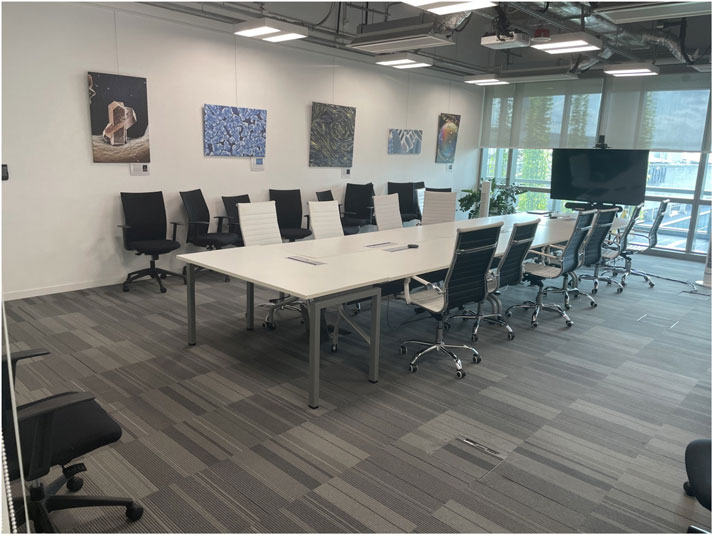
Figure 1. Visual description of the location of the different elements in the simulated room.

Figure 2

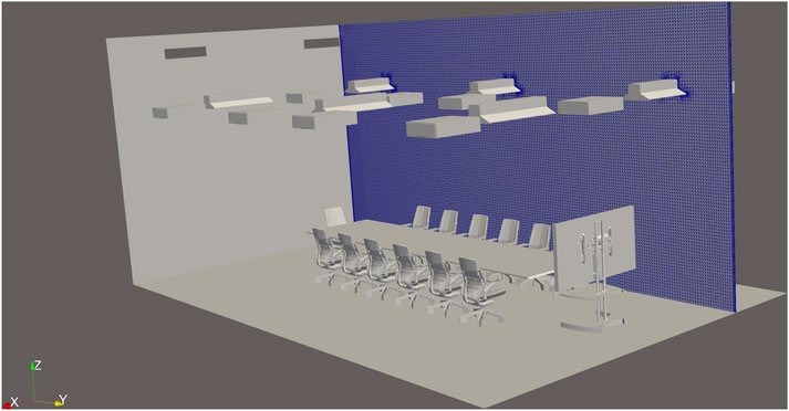
Figure 2. Mesh boundary and cut representation. Elements included are A/C inlets (trapezoidal shape hanging from the ceiling), light system (cuboidal shape hanging from the ceiling), chairs, tables and screen. Two return grilles used as outlets are in the upper part of the inner wall.

The 6 split A/C units in the room had a planar dimension of 120 × 59 cm and were spatially distributed as shown in the Figure 1. The air flow exhausted by the split unit was through 2 parallel and rectangular openings extending the size of the A/C unit. These openings were parallel to the glass wall of the room. Flow was ejected downwards 45 degrees with respect to ceiling/floor plane. Based on information provided by the Building Management Office, the A/C system was performing/calibrated to provide approximately 24 °C indoor air temperature. To reach this temperature each A/C unit worked in the following conditions:

The properties of walls are presented described in Section 2.2.1.

2.2 Physics-based model

2.2.1 Definition

The model representing the meeting room was designed to closely match the real-world dimensions and layout of the space, with a focus on preserving the geometrical accuracy of the elements that significantly influence airflow and thermal distribution.

The room geometry was created using Blender, guided by reference data from an iOS LiDAR scanning application (3D Scanner App). The scan (Figure 3) served solely as a visual and dimensional reference, while all critical architectural features, such as vent openings, inlet positions, and lighting points, were validated and adjusted using manual on-site measurements. A clean and accurately dimensioned geometry was then remodelled from scratch in Blender to ensure suitability for CFD simulation purposes.

Figure 3

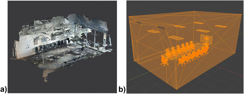
Figure 3. (a) Scan Mesh from 3D Scanner App and (b) Final mesh inside Blender.

To ensure a computationally tractable model, several simplifications were applied. In particular, the upper part of the air conditioning units, above the exhaust plane, was simplified given its minimal impact on the downward airflow dynamics. The complex volume of air above the A/C units, containing internal mechanical components (e.g., pipes of chilled water), was modelled as a porous medium to approximate its flow resistance. This way we reduced the complexity of the mesh and the number of cells, reducing computational cost of the simulations. However, the porous medium approach was not validated, and thus the results of the physical modelling apply to the occupied zone below the inlets, with possible deviations above 3.2 m (i.e., in the porous region). Figure 2 provides an overview of the final geometric model used in the simulation.

The entire project’s simulations were conducted using OpenFOAM, a widely used open source CFD framework (Weller et al., 1998). The geometry of the room was extracted and subsequently processed to generate a numerical mesh using OpenFOAM’s built-in meshing utility, snappyHexMesh. This tool enables the generation of body-fitted, predominantly hexahedral meshes, and supports layered boundary refinement, which is critical for resolving near-wall gradients, particularly important for convective heat transfer modelling. Due to these characteristics and previous experience of the team in similar studies, a specific grid independence study was not carried out.

Given the use of a multi-region conjugate heat transfer solver (chtMultiRegionSimpleFoam, see Section 2.2.2), the computational domain was divided into distinct mesh regions, each corresponding to either a fluid (air) or solid material domain. The mesh regions include: Air (fluid region), Ceiling, Concrete East Wall, Concrete West Wall, Glass North Wall, Glass South Wall and Floor.

Table 1 summarizes the cell counts in each region, demonstrating the high resolution used in the air region to capture detailed flow and temperature gradients. The characteristics of the mesh in the air region are: Max Non-orthogonality: 65; Average Non-orthogonality: 7.88; Min volume = 1.66e-08 m³; Max volume = 1.68e-04 m³; Total volume = 300.75 m³.

Table 1

Table 1. Number of cells in the mesh.

The solid regions were constructed via extrusion of surface meshes derived from triangulated wall surfaces. Each solid mesh comprises 10 layers, with a progressive expansion ratio to ensure adequate resolution of temperature gradients through the material thickness, while maintaining acceptable mesh quality metrics. Given the lower complexity of solving heat conduction in solids (as opposed to turbulence-resolving fluid flow), mesh quality requirements for the solid regions were relaxed compared to those in the air region.

Special attention was given to the generation of boundary layer meshes (inflation layers) in the air region to ensure that appropriate non-dimensional wall distance values (y+) were achieved (see Section 2.2.2). This enables accurate resolution of convective heat transfer using wall functions within the RANS framework (Stamou and Katsiris, 2006).

The solid regions were grouped into two primary material types, concrete and glass, each with distinct thermal properties such as thermal conductivity, specific heat capacity, and density. These material parameters are summarized in Table 2 (Cavanaugh and Speck, 2002; Crystran, 2020). To simplify, all solid envelopes were approximated to a thickness of 15 cm, including the glass walls. Thus, a single equivalent homogeneous layer was used with properties that reproduced the measured interior surface temperatures.

Table 2

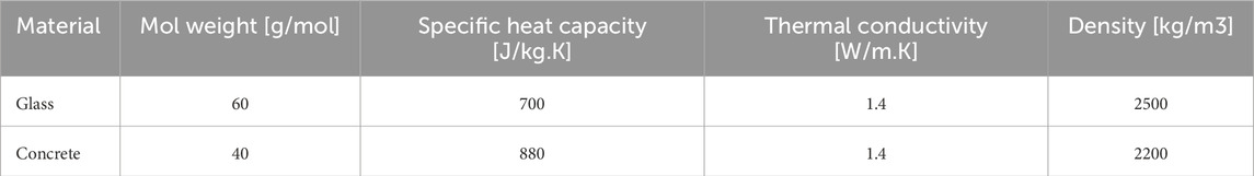
Table 2. Parameters of materials used.

2.2.2 Numerical approach and assumptions

Following the meshing phase, the simulation of the thermal and fluid dynamic behaviour of the meeting room was carried out using the chtMultiRegionSimpleFoam solver from the OpenFOAM framework. This solver is specifically designed to handle steady-state conjugate heat transfer problems across multiple regions, making it well-suited to simulate both the airflow within the room and the thermal conduction through solid surfaces such as walls, ceilings, and light fixtures. CFD-based studies of HVAC performance are a well-established discipline, frequently employed to guide the sizing and placement of air conditioning units (Kokash et al., 2022; Sarma and Jakhar, 2016) or to assess thermal comfort in occupied spaces (Buratti et al., 2017). In this work, however, such a modelling approach is not an end in itself but rather a foundation: the high-fidelity CFD simulations serve as the reference layer upon which reduced-order and hybrid models can be built, enabling fast yet physically consistent predictions that go beyond traditional HVAC design applications.

The choice of a steady-state solver is motivated by the nature of the problem: the goal is to capture the room’s thermal and flow conditions after a prolonged period of air conditioning operation, representative of equilibrium conditions typically observed during regular occupancy hours. As such, transient effects during start-up or occupant entry were not considered in this study.

In the air region, a Reynolds-Averaged Navier–Stokes (RANS) approach is adopted, using the k–ω Shear Stress Transport (SST) turbulence model. This formulation was chosen for the closure of the RANS equations because it combines a near-wall k–ω behaviour with improved free-stream robustness away from walls, making it well suited for indoor diffuser jets that exhibit strong shear layers and moderate buoyancy-driven stratification. This model provides a good balance between accuracy and computational cost for indoor airflow applications (Gangisetti et al., 2016). For near-wall treatment we used a mesh with inflation layers and targeted a low y⁺ so that the SST model could resolve the viscous sublayer where possible. An example of y⁺ per patch can be found in Table 3. These values reflect a predominantly low y⁺ mesh on most interior surfaces, while a subset of surface locations, mainly beneath strong impinging jets and outlets, exhibit larger local y⁺ due to high local velocities. In OpenFOAM, the used wall functions automatically adapt their formulation depending on the local y⁺ value, resolving the viscous sublayer when y⁺ is low and applying a logarithmic wall function when y⁺ lies in the log-layer range. This ensures consistent treatment across all wall regions despite local variations in mesh resolution and flow conditions.

Table 3

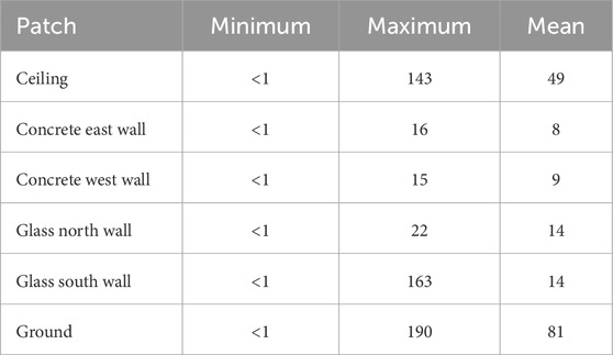
Table 3. Typical y + values in the considered mesh.

For the solid regions, a purely conductive heat transfer model is employed. Material properties for each region, as detailed in Table 2, were used to define thermal conductivity, density, and specific heat capacity. The inner surfaces of the solids, in contact with the air region, are thermally coupled through boundary conditions that incorporate temperature continuity and wall heat flux continuity. The outer surfaces of the building envelope are constrained using fixed-temperature conditions derived from in situ surface temperature measurements obtained via thermal infrared imaging (see Section 2.4). Based on these, the glass wall facing the outdoors had an external temperature of 32.9 °C, while the opposite wall (indoor) was 25.5 °C. For the other two concrete walls a value of 27.4 °C was considered as external surface boundary condition based on non-air-conditioned indoor areas of the building. This provides a realistic approximation of the interaction between the room and adjacent building spaces.

The conjugate heat transfer mechanism is resolved through tight coupling at the air-solid interfaces, using OpenFOAM’s generalized boundary conditions for temperature and turbulent heat transfer. To ensure adequate resolution of thermal gradients near walls and to improve numerical stability in the solid regions, inflation layers were applied at all air-solid boundaries during mesh generation.

Minor internal heat sources were also considered in the model. Specifically, the heat gain from the lighting fixtures was approximated and introduced as a surface heat source within the air region.

The air conditioning system is represented with a simplified geometric model of the diffuser and ducting. As described in Section 2.1, air is introduced into the room through six ceiling-mounted vents, which mimic the actual A/C inlets. The airflow enters through a modelled duct and diffuser arrangement that directs air jets at approximately 45° angles from the vertical, in line with the observed behaviour of the real system. Outlet boundary conditions are defined at the locations of the return grilles (see Figure 2), under the assumption that the door remains closed during operation.

Solar radiation effects were considered in the boundary condition selection process. However, based on site observations, direct solar radiation only affects the room indirectly during early morning hours (before 9:00 AM), while diffuse solar radiation is significantly attenuated by adjacent corridor glazing. Therefore, the direct contribution of solar gains to the indoor thermal environment was deemed negligible and excluded from the model.

Overall, the boundary conditions used for this study combine empirical data and realistic simplifications. The model was constrained using only the external surface temperatures measured outside the simulation domain (Section 2.4). Together with detailed material properties (Table 2), the numerical solver resolves the heat fluxes through the building envelope with sufficient fidelity for the purpose of Reduced-Order Model (ROM) generation (Section 2.3).

2.3 Surrogate model

After the physics-based simulation framework (Section 2.2) was fully established and validated, the process of generating data to train a surrogate model was undertaken. The objective was to construct a ROM capable of reproducing the thermal and airflow behaviour of the room under varying air conditioning settings, with significantly lower computational cost than full CFD simulations. In this study, the ROM approach was based on Proper Orthogonal Decomposition (POD), a method that extracts dominant spatial modes from the high-fidelity simulation data (Chinesta et al., 2025). These modes capture the most energetic and representative features of the flow and temperature fields. For any new input condition, the A/C system response will be reconstructed by interpolating the corresponding modal coefficients, thus enabling fast and accurate predictions over a wide range of scenarios.

2.3.1 Design of experiment

To ensure that the surrogate model captures the relevant dynamics of the A/C system with sufficient accuracy, an appropriate Design of Experiment (DoE) was defined. The purpose of the DoE is to sample the parameter space effectively, balancing the need for precision with the practical constraints of computational cost.

Sampling strategies aim to distribute sample points efficiently across the input domain, especially in higher-dimensional spaces. Various approaches exist, such as Latin Hypercube Sampling (Torregrosa et al., 2024), which ensure good coverage with limited samples. In this study, however, only two input parameters were considered, and the system response was expected to be relatively smooth. For this reason, a simple uniform grid sampling was adopted as a first step, which proved sufficient for the intended purpose.

The two independent parameters selected as primary control variables were the inlet air temperature and the air velocity at the A/C diffuser nozzle. Both correspond directly to adjustable settings of the physical A/C system and represent the main actuators available in the building management system. These variables play a decisive role in shaping both thermal comfort and energy consumption within the room.

Based on discussions with the building management team, the following parameter ranges were selected:

• Inlet temperature: from 17.8 °C to 23.8 °C, sampled at four evenly spaced points.

• Inlet velocity: from 0.1 m/s to 2.1 m/s, sampled at eleven evenly spaced points.

These values encompass the operational capabilities of a typical commercial air conditioning unit installed in the building, while also including the nominal setpoint provided by the building management system (22 °C and 1.1 m/s as shown in Table 4).

Table 4

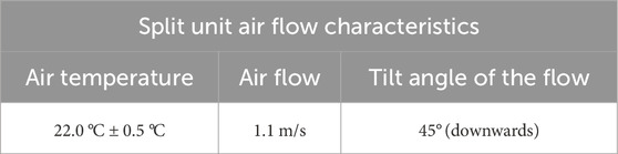
Table 4. Operation conditions of all the A/C units in the room.

By generating the full DoE, a total of 44 distinct simulation cases were defined. Each case represents a unique combination of the two control parameters and was simulated using the numerical CFD setup described in Section 2.2.

2.3.2 Reduced-order model (ROM) generation

Upon completion of the Design of Experiment (DoE) simulations, the resulting high-fidelity data were extracted and post-processed to construct the surrogate model. These simulation outputs, commonly referred to as snapshots, consist of the spatial distributions of two primary fields: air temperature and velocity within the room. Each snapshot corresponds to a unique combination of air inlet temperature and velocity as defined by the DoE.

To enable fast and accurate approximations of the A/C system’s behaviour under varying input conditions, a non-intrusive ROM was used. The method is based on POD, a widely used technique for model order reduction in fluid dynamics and heat transfer problems. POD identifies the dominant spatial structures, referred to as modes, present across the dataset, allowing the high-dimensional simulation outputs to be represented in a low-dimensional subspace.

This reduction is achieved by solving an eigenvalue problem on the snapshot matrix, yielding a set of orthonormal modes that optimally capture the energy content of the original fields. Each individual snapshot can then be reconstructed as a combination of these modes, weighted by a set of scalar modal coefficients specific to that parameter configuration.

Once the POD decomposition is complete, the next step involves establishing a relationship between the input parameters and the modal coefficients. In this study, a simple piecewise linear interpolation was employed for this purpose. Although more advanced interpolation schemes exist (Antoulas et al., 2022), the relatively dense and structured sampling used in the DoE allowed this approach to achieve sufficient accuracy for the intended application.

With the POD modes identified and the interpolation framework in place, the resulting surrogate model can predict the air temperature and velocity fields in the room for any new combination of input parameters within the defined range. This prediction process constitutes the online phase of the ROM and typically executes within a few milliseconds.

The overall ROM development process, including simulation, POD decomposition, and coefficient interpolation, is performed only once per setup and constitutes the offline phase. This phase incurs most of the computational cost, while the online phase provides fast, repeatable evaluations with minimal computational demand.

2.4 Experimental measurements

For the aim of providing suitable boundary conditions and validating the performance of the CFD and surrogate model, 2 types of sensors were used (Figure 4):

a. a. 3 sensors (Vaisala WXT536) were deployed throughout the room and outside the room providing data of air flow, air temperature and relative humidity. They were mounted on a tripod at a height of 1.2 m above the floor. 1-min records were stored in a datalogger (Scientific Campbell CR300).

b. b. A thermal infrared camera (RayThink RT630) was used to evaluate the surface temperature of the walls. A description of the sensors is provided in Table 5.

Figure 4

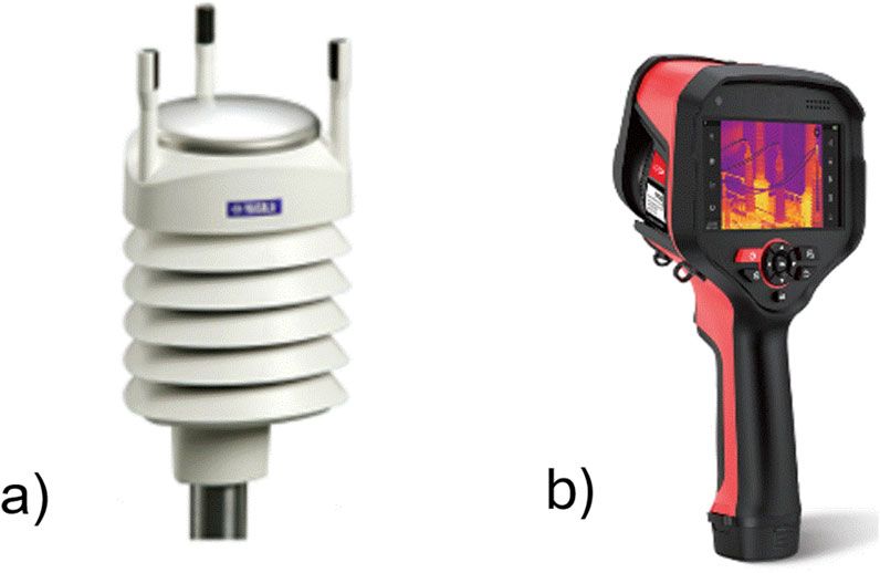
Figure 4. (a) WXT536 Transmitter (Vaisala), (b) RT630 Thermal Infrared Camera (RayThink).

Table 5

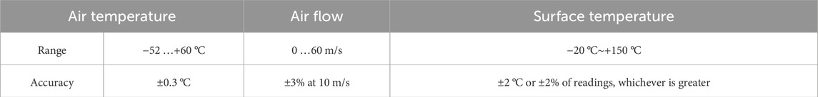
Table 5. Observation range and accuracy of the measurements.

The performance of the Vaisala WXT536 was evaluated inside the room by placing them one beside the other for 3 weeks. For air temperature, the highest mean bias error (MBE) was 0.064 °C). This value assures that the sensors can reflect small air temperature differences when distributed in different sites throughout the room.

For the evaluation of the air temperature and flow spatial distribution in the room, the sensors were deployed for 10 days, as shown in Figure 5.

Figure 5

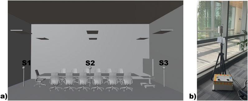
Figure 5. (a) Location of all sensors inside the room; (b) deployment of sensor S3 beside the outer glass wall.

Measurements of surface temperatures were done between 10:30 and 11:00. Different points/areas of the walls were evaluated, and a mean value was extracted as representative surface temperature of the wall. The measured data were used to fit the properties and physical parameters of each wall (Table 2). At the time these measurements were carried out indoor air temperature had little fluctuation, although it was slowly decreasing and adjusting from the night-time to the afternoon values. The A/C system started at 7 am and was running at a steady state (Table 4). Although the thermal and air flow were not fully stable, we did consider a steady state situation for modelling purposes.

2.5 Hybrid model

While the surrogate model provides accurate predictions for most of the domain, certain localized effects might not be fully captured. To address these discrepancies and improve overall predictive performance, a hybrid modelling approach was adopted, combining the surrogate model (section 2.3) with sparse experimental measurements (section 2.4) for targeted corrections (Figure 6).

Figure 6

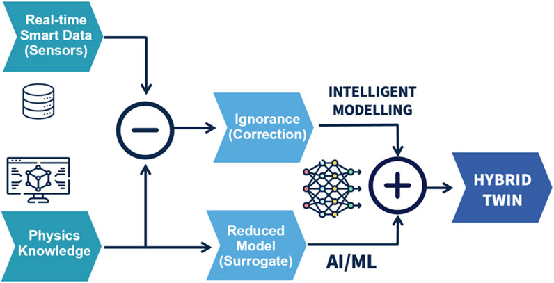
Figure 6. Schematic diagram for the hybrid mode consisting of a Surrogate model and ignorance/correction model based on the difference between the physics simulations and the real on-site measurements.

The correction strategy involves defining a new correction field representing the difference between the temperature field predicted by the surrogate model and the measured real-world temperature values at those points. It is then assumed that this correction field can itself be approximated as a linear combination of the previously extracted POD modes. This assumption is motivated by the fact that the original POD basis was generated from a wide range of simulation scenarios with diverse boundary conditions and flow patterns, suggesting that the correction field, while not directly in the snapshot set, lies within the span of these modes.

However, in the present case, only three measurement points were available in the room. A natural approach would be to use only three POD modes, yielding a fully determined linear system. Yet, practical experiments revealed that such a low-dimensional basis was insufficient to adequately represent the observed deviation. Instead, a larger basis of 30 POD modes was selected for the correction, offering more flexibility in representing the complex error field.

Given the underdetermined nature of this setup, three measurements versus 30 unknown modal coefficients, an iterative optimization approach was adopted. Specifically, a gradient descent algorithm was used to minimize the error between the corrected model and the sensor readings, iteratively adjusting the modal coefficients through a first loss function.

To ensure that the correction remains physically plausible and consistent with the expected flow structure, an additional regularization term was introduced into the loss function. This term penalizes deviations from the simulated case based on the setup while measuring (Section 2.2 and 2.3). Since the simulation corresponding to the sensor input parameters was possible, even if not fully accurate, it was assumed that the overall flow structures and large-scale temperature patterns were reasonably representative. The goal was to enforce that the corrected field maintains this general structure while allowing localized corrections based on sensor data.

The total loss function thus comprises two components:

• A sensor fitting term, minimizing the difference between corrected field values and measured temperatures at the sensor locations.

• A physics regularization term, minimizing the L2 norm (or Euclidian Norm) between the corrected field and the original simulated prediction.

These two terms are balanced using a scalar weight parameter α, which acts as a passive scalar to control the trade-off between data fidelity and physical structure consistency. A smaller α emphasizes fitting to sensor data, while a larger α preserves the original surrogate field structure. For the current study, a value of α = 0.5 was selected (see Section 3.3). This value was found to deliver satisfactory results for the hybrid model outcomes.

Thus, the correction process for the hybrid model is formulated as a constrained minimization problem, where the goal is to identify the optimal set of POD coefficients that minimize a combined loss function (L_total) incorporating both sensor alignment and physics-based regularization (Equation 1). The full formulation of this objective function is provided in Equation 1, where T_hybrid represents the corrected temperature field of the hybrid model, T_surrogate the prediction from the surrogate model, and T_simulated the reference field obtained from the high-fidelity simulation under the measurement conditions. The corrective field ΔT_correction is expressed as a linear combination of the extracted modes θ_i from the surrogate model, weighted by the unknown coefficients c_i to be determined.

The optimization of the POD coefficients was performed using the Adam optimizer, a stochastic gradient-based optimization method. The learning rate (step size) was set to 0.1, and the optimization was run for 5,000 iterations. No explicit stopping tolerance was imposed beyond this fixed iteration limit, as convergence of the loss was typically observed well before reaching 5,000 steps. Although the optimization problem is relatively simple and could be solved with standard gradient descent, Adam was chosen for its robustness and stable convergence behaviour without requiring manual tuning of momentum or step-size schedules.

$T_{hybrid}\left(x\right)=T_{surrogate}\left(x\right)-{\Delta T}_{correction}\left(x\right)(1)$

${\Delta T}_{correction}\left(x\right)={\displaystyle \sum _{i-0}^{N_{modes}}}{c}_i{\theta }_i\left(x\right)$

$L_{total}=\alpha L_{sensor}+\left(1-\alpha \right)L_{field}$

$L_{sensor}={‖T_{hybrid}\left(x_{sensor}\right)-T_{sensor}\left(x_{sensor}\right)‖}^2$

$L_{field}={‖T_{hybrid}\left(x\right)-T_{surrogate}\left(x\right)‖}^2$

3 Results and discussion

3.1 Outcomes of the sensors

Figure 7 shows the temporal evolution of the air temperature in the room throughout the campaign. Records show a clear pattern driven by the A/C system, following its operating hours. During daytime, air temperature in the room is ∼23.2 °C with an amplitude of ∼1 °C between the hottest and coldest sites inside the room. During the evening, when A/C is switched off, air temperature in the room tends to be homogenized (negligible spatial differences) increasing up to ∼27 °C just before the A/C system starts the following morning. This diurnal cycle is quite constant throughout the measurement period except during the weekend when the A/C system is not working.

Figure 7

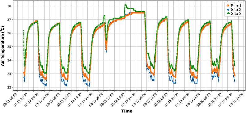
Figure 7. Temporal evolution of the air temperature in the room throughout the campaign.

Table 6 presents some statistical results of the air temperature records between 10:30 and 11:00 am (excluding the weekend period). Results show that the site close to the glass wall facing the outdoor corridor (S3) was the warmest with a difference of 0.6 °C with respect to the opposite glass wall facing the indoor corridor (S1). The lowest air temperature was in the centre of the room (S2), 1.1 °C lower than S3. During this period of the day, air temperature registered at each sensor was quite stable. The highest amplitude of values (1.1 °C) was in the site close to the outdoor corridor (S3) due to the influence of the conditions outside the building.

Table 6

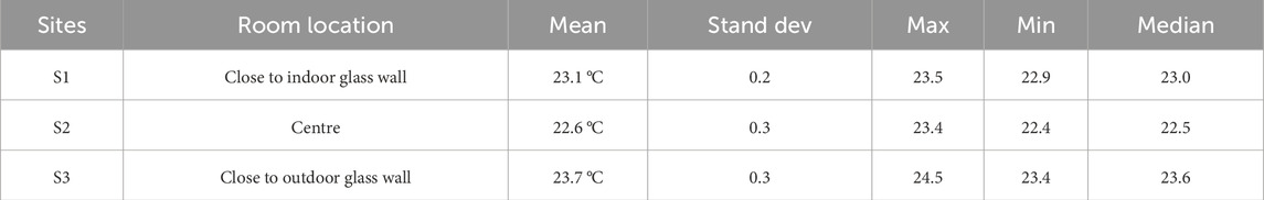
Table 6. Air temperature (°C) in the measuring sites inside the room between 10:30 and 11:00 am (without weekend).

Measurements of surface temperature using the thermal camera are presented in Table 7.

Table 7

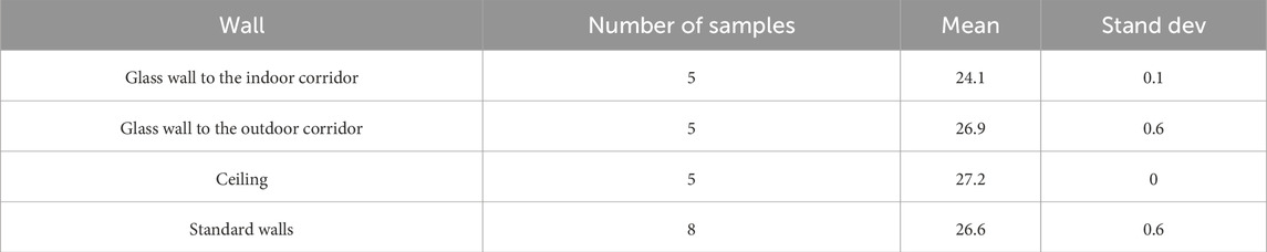
Table 7. Mean surface temperature (°C) of the interior walls of the room between 10:30 and 11:00 a.m.

3.2 Validation of the physics-based model

The steady-state simulation of the existing boundary conditions and the operating conditions of the A/C system was validated using measurement data collected between 10:30 and 11:00 a.m., a time window during which room conditions were stable and representative of equilibrium operation.

Table 8 presents a comparison between measured values and simulated outputs at key locations within the room. These include air temperature, and surface temperature measurements taken both inside and outside the simulated domain. Notably, surface temperatures were obtained using a thermal infrared (IR) camera, and air-related quantities were recorded using calibrated sensors.

Table 8

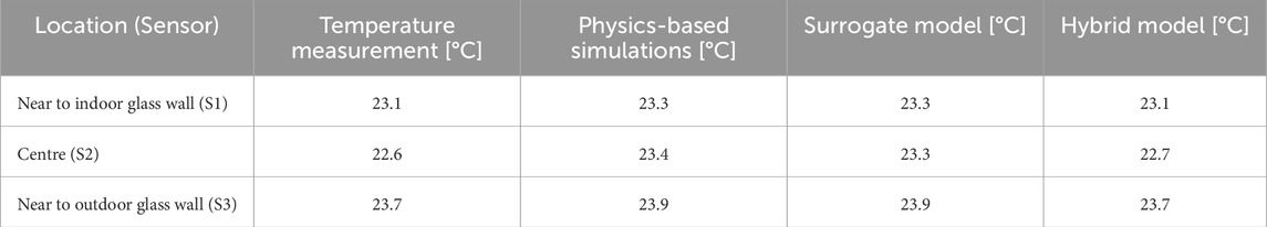
Table 8. Comparison of measurements inside the room with different models.

Despite the model using only the external surface temperatures measured as boundary conditions, the simulation was able to reproduce interior surface temperatures that match the IR camera measurements, providing confidence in the accuracy of the modelled wall conduction and convective coupling with the air domain. Figure 8 displays an example of the validation conducted on the wall within the room.

Figure 8

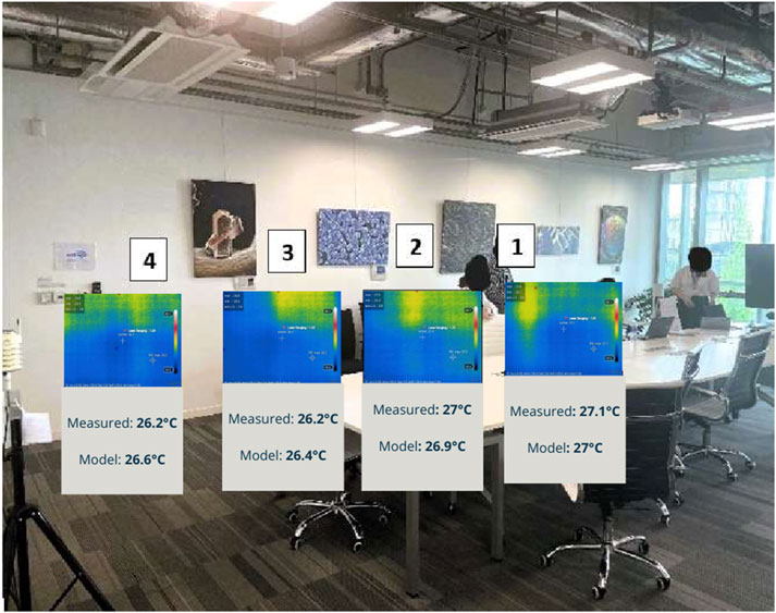
Figure 8. Example of the physics-based model validation: measurements vs. modelled surface temperature inside the room.

Overall, the results demonstrate satisfactory agreement between the steady-state simulation and the experimental observations, both surface and air temperature. This supports the validity of the physics-based model and its capacity to capture the dominant thermal and fluid phenomena within the room.

3.3 Performance of surrogate and hybrid model

The performance of the derived surrogate model is assessed by comparison with the observed temperature data (Table 8). Overall, the surrogate model demonstrates strong agreement with measured values, confirming its capacity to capture the dominant thermal behaviour of the room. However, a notable discrepancy was observed in the central area of the room, where the model fails to capture the local temperature drop. This discrepancy is aligned with the fact that the physics-based model (training data) cannot represent this localized phenomenon and thus neither can the reduced-order model.

By introducing a hybrid modelling approach, which integrates sparse sensor data into the surrogate prediction, we are able to correct this discrepancy. The hybrid model, after calibration using the sensor data and regularized optimization, significantly improves the temperature prediction in the central region. Additionally, the model also refines the temperature estimates at the other two sensor locations, reducing residual errors while preserving the overall structure of the temperature field.

These results clearly demonstrate the superior accuracy of the hybrid model, particularly in the central region where the largest error was previously observed. The hybrid approach effectively bridges the gap between model-based prediction and empirical observation, without overfitting to the sparse measurement set.

For our case study, the use of only three sensors seems enough since the deviation with respect to the sensors was moderate. In the case of larger deviations, it might be necessary to include more sensors or extend the spatial coverage of these (changing positions) in order to have more data to enable richer approximations.

Results presented in the Table 7 use a regulation weight α of 0.5, balancing the fit between sensor data and the preservation of the expected physical features of the flow field from the surrogate model (Section 2.5). To highlight the hybrid model’s sensitivity to this parameter, Figure 9a illustrates the evolution of the predicted temperature values at the three sensor locations as a function of α, while Figure 9b presents RMSE (including all sensors) as a function of α, showing that α = 0.5 can be considered the point on the curve where the improvement starts to level off. Beyond this point, increasing α further gives less gains while the physical structure/features of the flow could be affected. While the best results are obtained for α = 0.9 (RMSE = 0.030 °C), α = 0.5 achieves an acceptable RMSE = 0.087 °C.

Figure 9

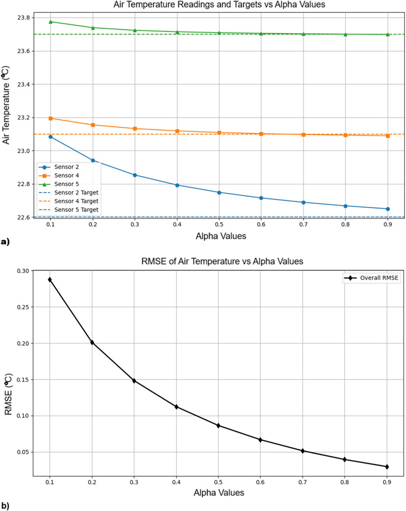
Figure 9. Effect of alpha on (a) air temperature at measuring sites, and (b) RMSE (considering the average measured values in the validation period (Table 6) of all the measuring sites). Higher values of alpha indicate the hybrid model getting closer to the sensor measurements but will diminish features of the spatial distribution of air temperature (Figure 10).

Figure 10 further provides a spatial visualization through a cut in the domain, of the temperature field, showing how different values of α influence the overall shape and intensity of the correction field.

Figure 10

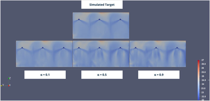
Figure 10. Representation of the simulated air temperature (°C) target and effect of α on the reconstructed field. Higher values of α will match better the measurements of the sensors (Figure 9) but the spatial distribution of air temperature will diverge from the target simulation. The opposite will occur with low values of α.

3.4 Spatial distribution of air temperature and flow

With the hybrid model now established, it becomes possible to simulate and visualize air temperature and flow patterns across different A/C operating conditions defined by the DOE, with response times in the order of milliseconds.

To demonstrate the model’s capabilities, several representative scenarios are presented, covering extreme operating conditions.

In the first case, the air conditioning system operates at its lowest settings, with minimal inlet velocity and the lowest supply temperature. Under these conditions, the system introduces little forced convection into the space. The resulting flow pattern is largely governed by natural convection and thermal stratification. A vertical gradient in air temperature is observed (Figure 11a), illustrating the tendency of warmer air to rise and cooler air to remain near the floor. The area directly below the A/C does show a cooler zone, but the system struggles to cool down the room.

Figure 11

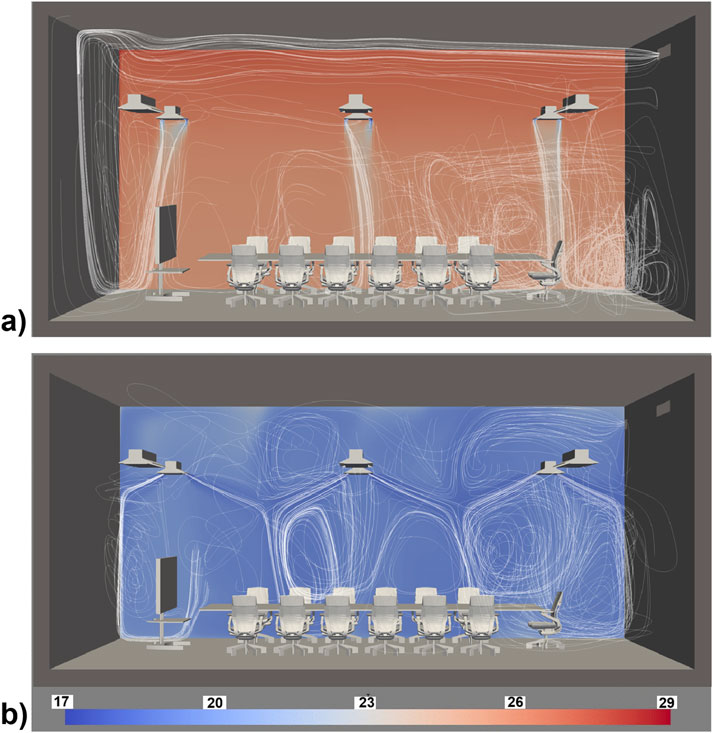
Figure 11. Visualisation of the spatial distribution of air temperature (°C) and air movement (streamlines) provided by hybrid model when the A/C work in different conditions (a) lowest speed (0.1 m/s) and temperature (17.8 °C), and (b) highest speed (2.1 m/s) and lowest temperature (17.8 °C).

At the opposite end of the operating range, maximum inlet velocity and lowest air temperature, the flow is dominated by strong forced convection. The air temperature field becomes more homogenized, with significantly reduced stratification (Figure 11b). Notably, localized cold spots appear near zones directly impacted by the cold air jet, particularly around the walls and floor around the supply diffusers, and where the diffuser’s flow impact each other’s.

These examples illustrate how the hybrid model, in combination with the real-time interface, can provide valuable insights into the spatial dynamics of indoor climate control, supporting both analysis and design optimization for air-conditioned spaces.

4 Conclusion

This study introduces and tests a hybrid modelling framework for predicting airflow and thermal conditions in a meeting room equipped with multiple A/C split units. The approach combined a high-fidelity multi-region CFD model, a ROM derived via POD, and sparse in situ measurements to enhance accuracy.

The physics-based model, validated against measured air and surface temperatures (at occupant level), provided a reliable baseline representation of the thermal and flow behaviour. However, the model was not validated for upper region of the meeting room where a porous medium was considered. The ROM, built from a limited set of only 44 high-fidelity simulations, delivered millisecond-scale predictions while closely matching most experimental data. However, certain localised phenomena, such as the observed central temperature drop, remained beyond the reach of the surrogate alone.

The hybrid approach addressed these limitations by integrating just three temperature sensors into the correction process. Despite the sparsity of both the training simulations and the measurement set, the method significantly reduced residual errors, restored the missing local temperature feature, and improved accuracy across all monitored points, while preserving physically plausible flow structures. However, a thorough validation of the model using independent measuring sites was not carried out, being this a limitation of the study and a task to consider in the future.

While the present formulation employs a global L2 regularisation term to constrain corrections, further improvement could be achieved by adopting more localised error metrics, such as norms computed via convolution kernels, to better capture and correct spatially confined discrepancies.

Overall, the results highlight that real-time, and physically consistent indoor climate predictions can be achieved with minimal simulation effort and sparse sensor deployment when coupled with a robust hybrid modelling framework.

Although this study focuses on a case study in Singapore, the methodology can be applied to different building types, climates and A/C systems by including in the hybrid model the relevant parameters that govern the variables to be simulated.

Data availability statement

The raw data supporting the conclusions of this article will be made available by the authors, without undue reservation.

Author contributions

BH: Writing – original draft, Writing – review and editing, Conceptualization, Formal Analysis, Investigation, Methodology, Validation, Visualization. JA: Conceptualization, Investigation, Methodology, Supervision, Validation, Visualization, Writing – original draft, Writing – review and editing. ZK: Data curation, Software, Visualization, Writing – original draft. FC: Conceptualization, Funding acquisition, Methodology, Supervision, Writing – review and editing.

Funding

The authors declare that financial support was received for the research and/or publication of this article. This research is part of the programme DesCartes and is supported by the National Research Foundation, Prime Minister’s Office, Singapore under its Campus for Research Excellence and Technological Enterprise (CREATE) programme.

Conflict of interest

The authors declare that the research was conducted in the absence of any commercial or financial relationships that could be construed as a potential conflict of interest.

Generative AI statement

The authors declare that no Generative AI was used in the creation of this manuscript.

Any alternative text (alt text) provided alongside figures in this article has been generated by Frontiers with the support of artificial intelligence and reasonable efforts have been made to ensure accuracy, including review by the authors wherever possible. If you identify any issues, please contact us.

Publisher’s note

All claims expressed in this article are solely those of the authors and do not necessarily represent those of their affiliated organizations, or those of the publisher, the editors and the reviewers. Any product that may be evaluated in this article, or claim that may be made by its manufacturer, is not guaranteed or endorsed by the publisher.

References

Antoulas, A. C., Beattie, C. A., Gugercin, S., and Gugercin, S. (2022). Interpolatory methods for model reduction [Bookshelf]. IEEE Control Syst. 42, 68–69. doi:10.1109/MCS.2022.3209060

CrossRef Full Text | Google Scholar

Bamodu, O., Xia, L., and Tang, L. (2017). “A numerical simulation of air distribution in an office room ventilated by 4-Way cassette air-conditioner,” in Energy procedia. doi:10.1016/j.egypro.2017.03.722

CrossRef Full Text | Google Scholar

Buratti, C., Palladino, D., and Moretti, E. (2017). “Prediction of indoor conditions and thermal comfort using CFD simulations: a case study based on experimental data,” in Energy procedia. doi:10.1016/j.egypro.2017.08.130

CrossRef Full Text | Google Scholar

Cavanaugh, K., and Speck, J. F. (2002). Guide to thermal properties of concrete and masonry systems reported by ACI committee. Concrete 122.

Google Scholar

Chappells, H., and Shove, E. (2005). Debating the future of comfort: environmental sustainability, energy consumption and the indoor environment. Build. Res. Inf. 33, 32–40. doi:10.1080/0961321042000322762

CrossRef Full Text | Google Scholar

Chinesta, F., Cueto, E., Abisset-Chavanne, E., Duval, J. L., and Khaldi, F.El (2020). Virtual, digital and hybrid twins: a new paradigm in data-based engineering and engineered data. Archives Comput. Methods Eng. 27, 105–134. doi:10.1007/s11831-018-9301-4

CrossRef Full Text | Google Scholar

Chinesta, F., Cueto, E., Champaney, V., Ghnatios, C., Ammar, A., Hascoët, N., et al. (2025). A gentle introduction to data, learning, and model order reduction. Switzerland, Cham: Springer Nature. doi:10.1007/978-3-031-87572-4

CrossRef Full Text | Google Scholar

Crystran (2020). The crystran handbook of nfra-red and ultra-violet optical materials. J. Chem. Inf. Model.

Google Scholar

Fisk, W. J. (2015). Review of some effects of climate change on indoor environmental quality and health and associated no-regrets mitigation measures. Build. Environ. 86, 70–80. doi:10.1016/j.buildenv.2014.12.024

CrossRef Full Text | Google Scholar

Ford, B., Mumovic, D., and Rawal, R. (2022). Alternatives to air-conditioning: policies, design, technologies, behaviours. Build. Cities 3, 433–447. doi:10.5334/bc.256

CrossRef Full Text | Google Scholar

Freire, R. Z., Oliveira, G. H. C., and Mendes, N. (2008). Predictive controllers for thermal comfort optimization and energy savings. Energy Build. 40, 1353–1365. doi:10.1016/j.enbuild.2007.12.007

CrossRef Full Text | Google Scholar

Gangisetti, K., Claridge, D. E., Srebric, J., and Paulus, M. T. (2016). Influence of reduced VAV flow settings on indoor thermal comfort in an office space. Build. Simul. 9, 101–111. doi:10.1007/s12273-015-0254-3

CrossRef Full Text | Google Scholar

Goethals, K., Couckuyt, I., Dhaene, T., and Janssens, A. (2012). Sensitivity of night cooling performance to room/system design: surrogate models based on CFD. Build. Environ. 58, 23–36. doi:10.1016/j.buildenv.2012.06.015

CrossRef Full Text | Google Scholar

Gopaliya, M. K., Reddy Pulagam, M. K., and Kumari, N. (2021). “Comparative study of positioning of air conditioner in a room using cfd,” in Lecture notes in mechanical engineering. doi:10.1007/978-981-15-6360-7_15

CrossRef Full Text | Google Scholar

Hou, D., and Evins, R. (2024). A protocol for developing and evaluating neural network-based surrogate models and its application to building energy prediction. Renew. Sustain. Energy Rev. 193, 114283. doi:10.1016/j.rser.2024.114283

CrossRef Full Text | Google Scholar

Kjellstrom, T., and Crowe, J. (2011). Climate change, workplace heat exposure, and occupational health and productivity in central America. Int. J. Occup. Environ. Health 17, 270–281. doi:10.1179/107735211799041931

PubMed Abstract | CrossRef Full Text | Google Scholar

Kokash, H., Burzo, M. G., Agbaglah, G., and Mazumder, F. (2022). “Optimized hvac air distribution for improved air quality using cfd analysis,” in ASME international mechanical engineering congress and exposition, proceedings (IMECE). doi:10.1115/IMECE2022-95730

CrossRef Full Text | Google Scholar

Kummitha, O. R., Kumar, R. V., and Krishna, V. M. (2021). CFD analysis for airflow distribution of a conventional building plan for different wind directions. J. Comput. Des. Eng. 8, 559–569. doi:10.1093/jcde/qwaa095

CrossRef Full Text | Google Scholar

Liao, W., Peng, J., Luo, Y., He, Y., Li, N., and A, Y. (2022). Comparative study on energy consumption and indoor thermal environment between convective air-conditioning terminals and radiant ceiling terminals. Build. Environ. 209, 108661. doi:10.1016/j.buildenv.2021.108661

CrossRef Full Text | Google Scholar

Liu, W., He, Y., and Liu, Z. (2024). Indoor pollution control based on surrogate model for residential buildings. Environ. Pollut. 346, 123638. doi:10.1016/j.envpol.2024.123638

PubMed Abstract | CrossRef Full Text | Google Scholar

Luo, M., Wang, Z., Brager, G., Cao, B., and Zhu, Y. (2018). Indoor climate experience, migration, and thermal comfort expectation in buildings. Build. Environ. 141, 262–272. doi:10.1016/j.buildenv.2018.05.047

CrossRef Full Text | Google Scholar

Moise, A. F., Sahany, S., Hassim, M. E., Chen, C., Chua, X. R., Prasanna, V., et al. (2024). “Singapore’s third national climate change study,” in Climate change projections to 2100 (Singapore: Science Report).

Google Scholar

Morozova, N., Trias, F. X., Capdevila, R., Pérez-Segarra, C. D., and Oliva, A. (2020). On the feasibility of affordable high-fidelity CFD simulations for indoor environment design and control. Build. Environ. 184, 107144. doi:10.1016/J.BUILDENV.2020.107144

CrossRef Full Text | Google Scholar

Omer, A. M. (2008). Energy, environment and sustainable development. Renew. Sustain. Energy Rev. 12, 2265–2300. doi:10.1016/j.rser.2007.05.001

CrossRef Full Text | Google Scholar

Patel, A., and Dhakar, P. S. (2018). CFD analysis of air conditioning in room using ansys fluent. J. Emerg. Technol. Innov. Res. 5. doi:10.13140/RG.2.2.13462.50249

CrossRef Full Text | Google Scholar

Salamanca, F., Georgescu, M., Mahalov, A., and Moustaoui, M. (2015). Summertime response of temperature and cooling energy demand to urban expansion in a semiarid environment. J. Appl. Meteorol. Climatol. 54, 1756–1772. doi:10.1175/JAMC-D-14-0313.1

CrossRef Full Text | Google Scholar

Sarma, S., and Jakhar, O. P. (2016). Computational analysis of impact of the air-conditioner location on temperature and velocity distribution in an office-room. Int. Res. J. Eng. Technol. 3.

Google Scholar

Sharif, S. A., and Hammad, A. (2019). Developing surrogate ANN for selecting near-optimal building energy renovation methods considering energy consumption, LCC and LCA. J. Build. Eng. 25, 100790. doi:10.1016/j.jobe.2019.100790

CrossRef Full Text | Google Scholar

Singh, V. K., Mughal, M. O., Martilli, A., Acero, J. A., Ivanchev, J., and Norford, L. K. (2022). Numerical analysis of the impact of anthropogenic emissions on the urban environment of Singapore. Sci. Total Environ. 806, 150534. doi:10.1016/j.scitotenv.2021.150534

PubMed Abstract | CrossRef Full Text | Google Scholar

Stamou, A., and Katsiris, I. (2006). Verification of a CFD model for indoor airflow and heat transfer. Build. Environ. 41, 1171–1181. doi:10.1016/j.buildenv.2005.06.029

CrossRef Full Text | Google Scholar

Suarez-Gutierrez, L., Müller, W. A., Li, C., and Marotzke, J. (2020). Hotspots of extreme heat under global warming. Clim. Dyn. 55, 429–447. doi:10.1007/s00382-020-05263-w

CrossRef Full Text | Google Scholar

Tian, W., Han, X., Zuo, W., and Sohn, M. D. (2018). Building energy simulation coupled with CFD for indoor environment: a critical review and recent applications. Energy Build. 165, 184–199. doi:10.1016/j.enbuild.2018.01.046

CrossRef Full Text | Google Scholar

Torregrosa, S., Champaney, V., Ammar, A., Herbert, V., and Chinesta, F. (2024). Physics-based active learning for design space exploration and surrogate construction for multiparametric optimization. Commun. Appl. Math. Comput. 6, 1899–1923. doi:10.1007/s42967-023-00329-y

CrossRef Full Text | Google Scholar

Weller, H. G., Tabor, G., Jasak, H., and Fureby, C. (1998). A tensorial approach to computational continuum mechanics using object-oriented techniques. Comput. Phys. 12, 620–631. doi:10.1063/1.168744

CrossRef Full Text | Google Scholar

WHO (2004). Heat-waves: risks and responses. Health Glob. Environ. Health Ser. No. 2, 124. doi:10.1007/s00484-009-0283-7

CrossRef Full Text | Google Scholar

Zhu, H., Hu, S., Wang, G., Han, L., Jing, M., and Zhao, X. (2023). Full-scale numerical simulation and experimental validation of the thermal environment under the heating mode in an air-conditioned room. Case Stud. Therm. Eng. 51, 103548. doi:10.1016/j.csite.2023.103548

CrossRef Full Text | Google Scholar