Field application of BOFDA-based distributed fiber optic sensing in static load testing of cast-in-place pile foundations

Distributed fiber optic sensing (DFOS) offers a transformative approach for monitoring geotechnical structures by providing continuous, high-resolution strain profiles along pile shafts. In this study, a Brillouin optical frequency domain analysis (BOFDA) system was deployed to monitor seven trial cast-in-place piles subjected to vertical static load tests. Optical fibers arranged in dual U-shaped loops were embedded along the reinforcement cages, enabling detailed measurement of axial strain, load transfer, and side friction across different soil strata. Results indicate that side friction distributions captured by BOFDA generally fall below conservative site investigation values from site investigations, confirming the conservative nature of conventional design parameters. However, anomalies, such as localized overestimation of side friction in weathered sandstone, were observed in weathered sandstone layers and premature slippage near the pile head at high load levels. These behaviors highlight the sensitivity of BOFDA monitoring and the complex interplay between soil stratigraphy, pile–soil interface conditions, and applied loading. The study demonstrates that while current design practice remains safe, distributed sensing provides valuable diagnostic insights into localized side friction mobilization, supporting more refined design, improved construction quality control, and future integration of DFOS data into load-transfer modeling.

Introduction

Pile foundations, critical to modern infrastructure, require advanced monitoring to ensure safety and performance. With global infrastructure investments projected to reach 94 trillion USD by 2040 (New York Climate Week, 2024), failures of these systems—often linked to undetected defects, soil variability, or environmental loads—pose major technical and economic risks, with landslides alone causing losses of more than 10 billion USD annually (Minardo et al., 2021). Monitoring these underground “hidden” systems remains a significant challenge. Conventional tools, including strain gauges and inclinometers, provide only point-based information, are prone to electromagnetic interference, and often degrade under harsh field conditions (Bado and Casas, 2021). Such limitations restrict our ability to assess load transfer, deformation patterns, and ultimate capacity, thereby undermining the safety and durability of overlying structures (Guo and Zhao, 2018).

Recent advances in smart sensing technologies offer new opportunities for continuous and distributed monitoring. Distributed fiber optic sensing (DFOS), which relies on light scattering phenomena in optical fibers, enables the measurement of strain, temperature, and vibration over kilometers of fiber with centimeter-scale resolution (Ma et al., 2023; Lu et al., 2019). Compared with quasi-distributed or point sensors, DFOS is immune to electromagnetic interference, resistant to corrosion, and can be directly embedded into concrete, soil, or rock (Wu et al., 2023; Fu et al., 2023; Bado and Casas, 2021). Several configurations exist, such as Brillouin optical frequency domain analysis (BOFDA), which uses Brillouin scattering for high-resolution frequency-domain measurements, and optical frequency domain reflectometry (OFDR), which employs Rayleigh scattering to achieve sub-millimeter resolution (Bernini, Minardo, and Zeni, 2012; Ding et al., 2014; Garus et al., 1996; Schenato et al., 2017). These methods surpass earlier time-domain approaches such as Brillouin optical time-domain reflectometry (BOTDR) by providing finer resolution and faster acquisition, though often with trade-offs between range and resolution (Lu et al., 2019; Minardo et al., 2021).

Field applications of DFOS in geotechnics have expanded rapidly. BOFDA and BOTDR have been employed to detect precursory strains in flume tests of granular slopes and monitor fracture evolution in rock cliffs over multi-year periods (Schenato et al., 2017). Similarly, OFDR has enabled detailed profiling of strain in pile load tests, revealing side friction distributions and stiffness variations that conventional instrumentation could not resolve (Bado and Casas, 2021). Ongoing improvements in fiber coatings, anchorage methods, and signal processing further enhance coupling with geomaterials and reduce noise, while integration with machine learning holds promise for predictive geotechnical monitoring (Minardo et al., 2018; Ma et al., 2023).

This study investigates the use of BOFDA-based distributed fiber optic sensing in static load testing of cast-in-place pile foundations. Seven trial piles were monitored during staged vertical loading, with dual U-shaped armored fibers embedded in the reinforcement cages. Continuous strain profiles were acquired and used to derive axial forces and side friction distributions across multiple soil layers. By comparing the distributed measurements with recommended values from site investigations, this study evaluates both the feasibility and limitations of BOFDA monitoring in field pile testing. The results provide new insights into the mobilization of side friction, highlight the challenges of field fiber survivability, and suggest pathways for refining load-transfer models and improving construction quality control in pile foundation engineering.

Principles of BOFDA-based distributed optical fiber sensing technology

Principle

The BOFDA technique is based on Brillouin scattering, a nonlinear optical interaction between incident light and acoustic phonons in the fiber, which generates a frequency-shifted backscattered signal known as the Brillouin frequency shift (BFS) (Garus et al., 1996). The BFS is linearly related to local strain and temperature, allowing the fiber to function as a distributed sensor along its full length. As shown in Equation 1 (Bernini et al., 2012).

Figure 1 illustrates the BOFDA system setup, including pump and probe light interactions. Continuous-wave pump light from a narrow-linewidth laser is injected into one end of the fiber, while probe light is launched from the opposite end. The frequency difference between the pump and probe light is tuned to the BFS, typically approximately 13 GHz for standard single-mode fibers at a 1.3 μm wavelength. When resonance is achieved, energy exchange occurs via stimulated Brillouin scattering. The probe is amplitude-modulated through an electro-optic modulator (EOM), and the resulting interaction is captured using a photodetector. The detected signal is processed using a vector network analyzer and converted through an inverse fast Fourier transform (IFFT) to yield a distributed profile of strain or temperature along the fiber (Garus et al., 1996). Auxiliary components such as erbium-doped fiber amplifiers (EDFAs), polarization scramblers, and fiber Bragg gratings are commonly used to ensure signal fidelity.

Figure 1

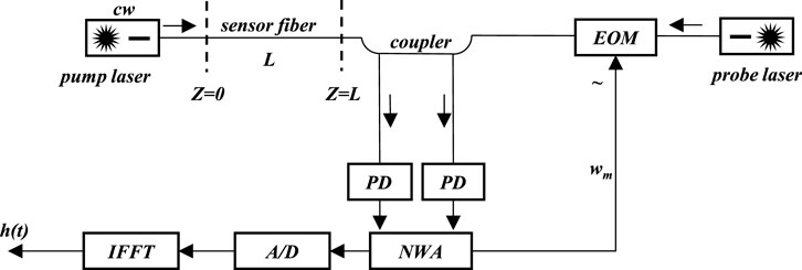
Figure 1. Principle of the BOFDA method (Garus et al., 1996).

The relationship between BFS (${\mathrm{\nu }}_{\mathrm{B}}$) and strain $\left(\mathrm{\epsilon }\right)$ or temperature ($\Delta T$) is given as follows:

$\left[{\mathrm{\nu }}_B={\mathrm{\nu }}_{B0}+C_{\mathrm{\epsilon }}\mathrm{\epsilon }+C_T\Delta T\right],$

where ${\mathrm{\nu }}_{B0}$ is the reference Brillouin frequency and $C_{\epsilon }$ and $C_T$ are the strain and temperature sensitivity coefficients, respectively (Lu et al., 2019).

Advantages and disadvantages

The BOFDA approach provides several advantages for geotechnical monitoring. Its frequency-domain configuration achieves centimeter-scale spatial resolution (typically 5–10 cm), far exceeding the meter-scale resolution of BOTDR. It also enables long-distance sensing over tens of kilometers, suitable for large infrastructure such as tunnels and foundations. The method is inherently less sensitive to noise than time-domain techniques and allows simultaneous strain and temperature monitoring. Field applications confirm its robustness; in this study, for example, metal-armored cables embedded in piles maintained a 78.6% survival rate through casting, chiseling, and pile-cap construction.

However, limitations remain. High sensitivity can result in jagged strain curves, particularly at soil layer interfaces where stress concentrations occur. The measurement setup requires multiple components (EDFA and polarization controllers), which increases system complexity and cost. Data reliability depends strongly on post-processing techniques such as denoising and curve smoothing, and stress concentrations at soil interfaces may exaggerate BFS readings, leading to overestimation of local strain. Finally, because BFS is sensitive to both strain and temperature, careful calibration is required to decouple these effects in field environments where thermal gradients may vary dynamically.

In situ testing

Project overview

The test site comprised two construction plots designated for high-rise residential development. The planned superstructure consists of tower buildings with heights not exceeding 100 m, supported by a frame–shear wall system, and is underlain by a two-story basement designed with a frame structure.

A total of seven trial piles were installed, detailed in Table 1, all designed as compression piles. Among them, four piles had a diameter of 1.2 m, and three piles had a diameter of 1.4 m. The pile locations are shown in Figure 2. The piles were constructed using C40 underwater concrete, with design characteristic vertical bearing capacities of 12,000 kN for the 1.2 m piles and 16,000 kN for the 1.4 m piles.

Table 1

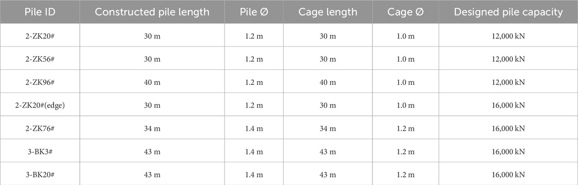
Table 1. Information on trial piles.

Figure 2

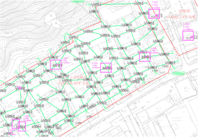
Figure 2. Layout of test piles.

This study investigates the application of BOFDA distributed optical fiber sensing technology in static load testing of cast-in-place pile foundations to assess pile behavior and side friction resistance distributions in homogeneous soil layers. The methodology encompasses experimental design, fiber optic cable selection and deployment, data acquisition procedures, and analytical methods for deriving axial forces and side friction resistances.

Engineering geology

According to the borehole investigation, the stratigraphy at the site (e.g., ZK1) comprises a sequence of Quaternary overburden underlain by Carboniferous bedrock sandstone. The soil and rock layers and their properties are summarized in Table 2.

Table 2

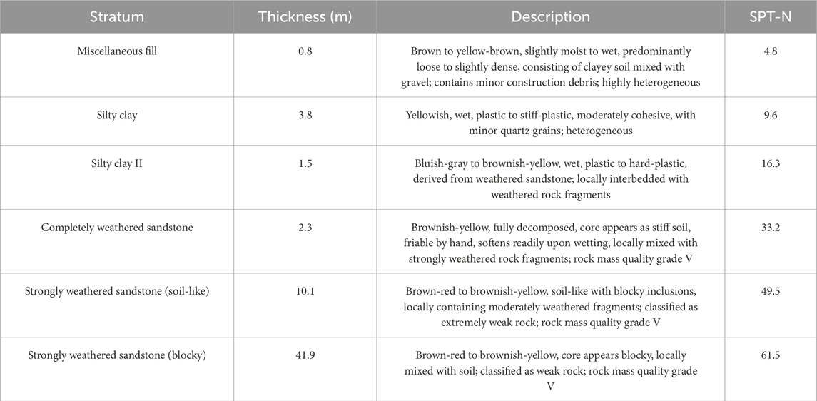
Table 2. Engineering geological characteristics at ZK1.

Static loading test setup

Vertical compression tests were conducted in accordance with the Technical Code for Testing of Building Pile Foundations (SJG 09-2020), as shown in Figure 3. The maximum applied load was at least twice the design characteristic capacity, with selected 1.2 m diameter piles (one grouted and one un-grouted) loaded to failure. Reaction systems combining anchor piles and counterweights were designed to provide a counterforce of no less than 1.2 times the maximum load, and pile heads were carefully prepared to ensure stability and integrity.

Figure 3

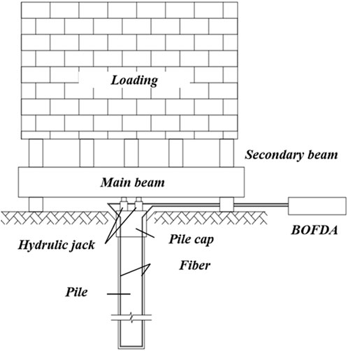
Figure 3. Schematic of the static load test.

Tests adopted the maintained load method at a rate of 0.1–0.2 mm/min, per SJG 09-2020. The load was applied in equal increments (with the first doubled) and maintained until settlement stabilized, defined as less than 0.1 mm per hour. Settlement was recorded at regular intervals using displacement transducers symmetrically arranged around the pile head. Unloading was performed in steps twice as large as the loading increments, followed by residual settlement monitoring.

Termination criteria included excessive settlement relative to the previous stage, non-stabilization after 24 h, attainment of large cumulative settlement, or reaching the maximum planned load. Test results were interpreted from load–settlement (Q–s) and settlement–time (s–log t) curves to determine the ultimate bearing capacity, consistent with the code provisions, and were determined automatically.

BOFDA sensing

Fiber selection

Commercially available strain-sensing fiber optic cables have been widely applied for monitoring deformation in reinforced concrete and geotechnical structures. Common types include unjacketed fibers, high strain-transfer tight-buffered cables, metal-armored strand-type cables, metal-armored tape-type cables, and fiber-reinforced plastic (FRP) single- and multi-core cables (Table 3).

Table 3

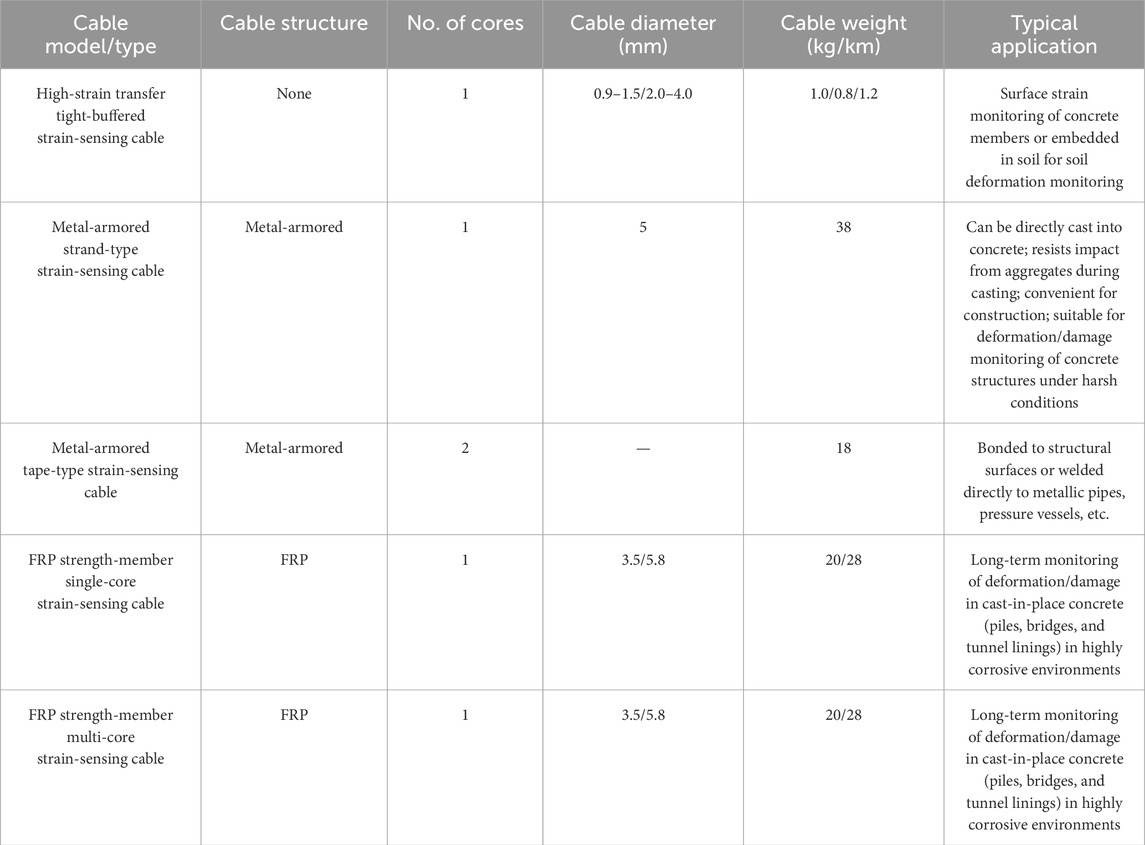
Table 3. Parameters of strain-sensing optical fiber cables.

Metal-armored strand-type cables were selected for this project (Figure 4), considering the construction process of cast-in-place piles, the need to resist impact during concrete casting, and the absence of long-term monitoring requirements. These cables provide robust protection against chipping, welding, and backfilling operations, although coordination among construction teams remains essential to prevent localized damage.

Figure 4

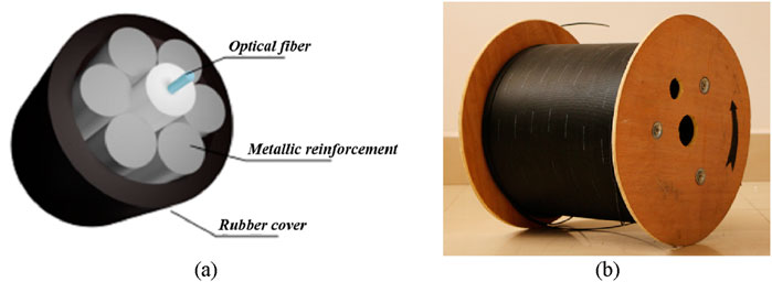
Figure 4. Metal-armored strand-type strain-sensing cables: (a) sectional view and (b) cable in reality.

Furthermore, considering the dual U-shaped layout and the splice allowance, the required cable length per pile is listed in Table 4.

Table 4

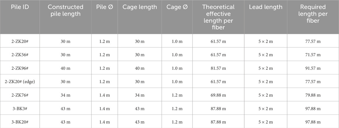
Table 4. Parameters for metal-armored strand-type strain-sensing cable.

In summary, the total theoretical cable length required for this project is 1,187.84 m. Due to additional lead allowances arising from bar-lifting welds, protective steel tubing, and other installation considerations, the actual lead lengths increased to varying degrees; the total actual cable used was approximately 1,250 m, which satisfies the testing requirements for this project.

Sensor installation

Each pile was instrumented with two optical fibers arranged in a dual U-shaped layout. Fibers were fixed to the primary reinforcement bars along the side to avoid direct contact with fresh concrete. The dual-loop configuration was adopted to increase survivability and provide redundancy for data validation. A schematic of the installation is shown in Figure 5. Protective measures were applied at the pile head, including steel sleeves, to minimize damage during head breaking. Integrity testing using red-light pens and fiber testers was performed at key stages to ensure continuity. The installation scheme is shown in Figure 5.

Figure 5

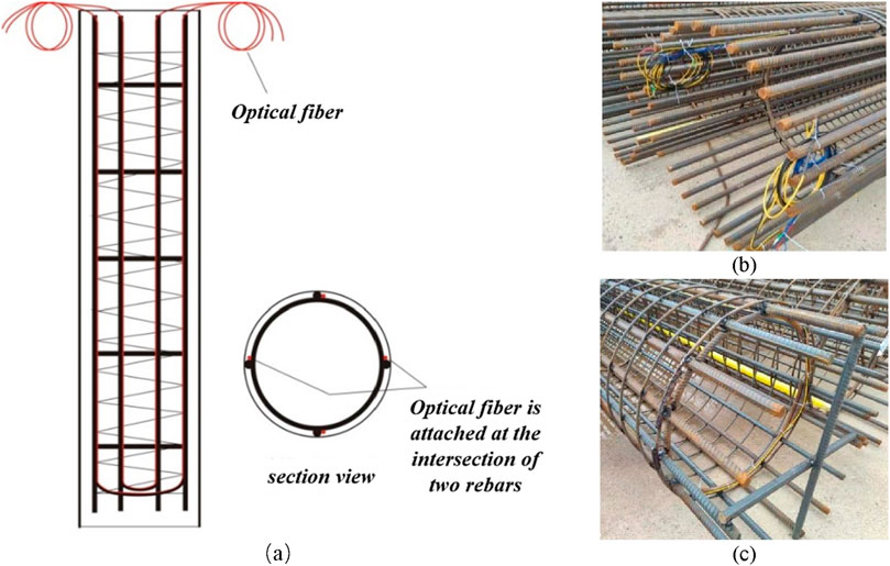
Figure 5. Schematic of DFOS fiber placement in the cast-in-place pile, where the yellow line is the fiber sensor. (a) Section view, (b) detailed view of the pile head, and (c) detailed view of the pile bottom.

The specific steps for deploying the sensors in the pile foundation are as follows:

Step 1 Fiber length preparation: An optical fiber cable of appropriate length, based on the pile specifications, must be prepared. The required cable length is calculated as follows:

$\text{Cable length}=\text{pile length}\times 2+\text{half the reinforcement cage}\text{circumference}+\text{lead}--\text{in length}\times 2$

Step 2 Initial fiber binding: The center of the optical fiber cable must be aligned with the bottom hoop of the lowest reinforcement cage section. The fiber along the inner side of the hoop must be bound, ensuring that it is securely fixed to the hoop and positioned away from areas likely to be impacted by concrete pouring equipment. Subsequently, the fiber along the inner side of the main load-bearing reinforcement bars of the cage must be secured using cable ties at intervals of 0.5–1.0 m. The exact spacing may vary due to the presence of denser hoops, depending on the on-site binding workspace.

Step 3 Reinforcement cage installation: After binding the optical fiber cable to the bottom reinforcement cage section, the cage must be lowered into the drilled hole and temporarily fixed in place. The remaining fiber cable must be straightened and positioned away from the welding zone of the reinforcement cage. Once the next cage section is welded in place, the fiber binding process must be repeated for the subsequent section.

Step 4 Pile top protection and integrity testing: At the pile top, the excess optical fiber cable must be protected using a steel sleeve to prevent damage during pile-head breaking. After pile casting and post-grouting are completed, the fiber connectors must be spliced. An integrity test must be performed using a red-light fiber pen or an optical fiber tester to ensure the fiber’s continuity and unobstructed signal transmission.

Step 5 Data acquisition preparation: Once the loading equipment is installed, lead-in cables must be deployed to connect the optical fiber with the BOFDA demodulator for testing.

Fiber splice bridging and integrity testing

After concreting and before chipping the pile head, FC-type fiber optic connectors were used to bridge the sensor leads at both the head and tail of each fiber, followed by an integrity test (Figure 6). The same procedure was applied to verify fiber integrity prior to pile-head chipping, pile-cap construction, and data acquisition.

Figure 6

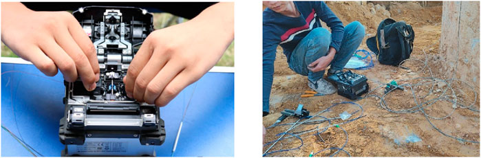
Figure 6. Fiber fusion splicing.

Fiber survivability checking

Although the metal-armored, strand-type strain-sensing cable protects the fiber with multiple metallic strength members, external impacts during construction—such as concrete casting and pile-head chipping (Figure 7)—can still cause damage. Fiber survivability, summarized in Table 5, was affected by construction activities (under the dual U-shaped layout, fibers are distinguished as Fiber #1 and Fiber #2).

Figure 7

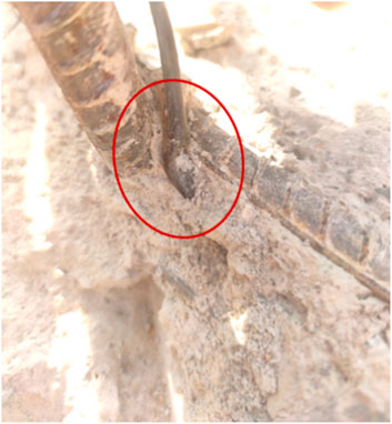
Figure 7. Fiber damage caused by chiseling.

Table 5

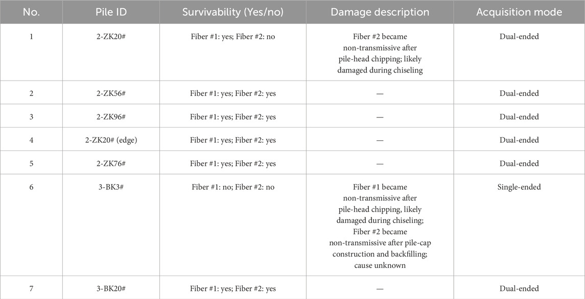
Table 5. Fiber survivability.

In total, 14 fibers were embedded across seven piles. Despite the protection afforded by the metal-armored design, three fibers were damaged during subsequent stages of concreting, pile-head chiseling, or pile-cap construction (Table 5). In pile 2-ZK20#, one fiber was lost after chiseling; in pile 3-BK3#, both fibers failed, although one provided 95 m of usable length and was applied in single-ended acquisition mode. The overall survivability rate was 78.6%, and the effective measurability reached 99.5%. These results demonstrate that while distributed sensing can be effectively applied in field pile testing, survivability remains sensitive to on-site handling, particularly at the pile head.

Data acquisition

Data were acquired using a BOFDA demodulator (Figure 8), which enabled high-resolution strain acquisition, as specified in Table 6. The system offers 0.05 m maximum sampling resolution, ±2 με strain accuracy, and a 50 km effective range, enabling high-density measurements along each pile. Acquisition parameters for each test pile are given in Table 7. During the staged static load tests, axial strain was recorded at each load increment, providing continuous strain profiles with more than 2,000 data points per pile. Work as shown in Figures 9–11.

Figure 8

Figure 8. Fiber tester for integrity verification.

Table 6

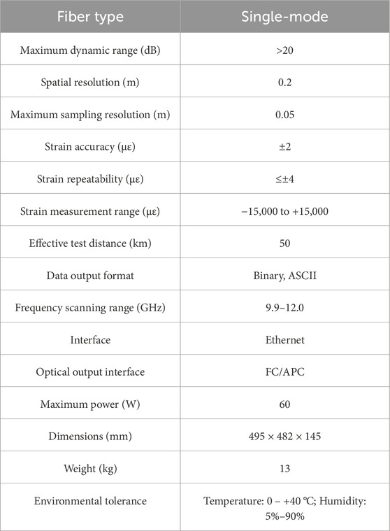
Table 6. Performance specifications of the demodulation apparatus.

Table 7

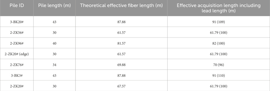
Table 7. Acquisition instruments and parameters for each pile.

Figure 9

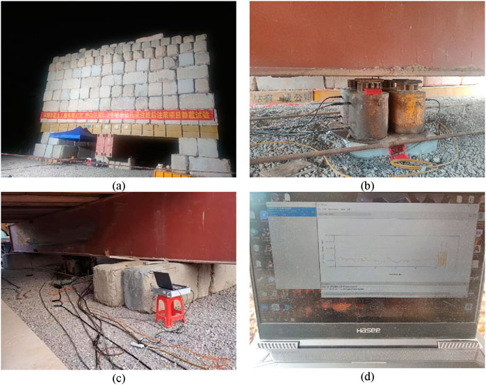
Figure 9. Site testing setup: (a) surcharge loading setup, (b) hydraulic jack, and (c) and (d) data acquisition (during test).

Figure 10

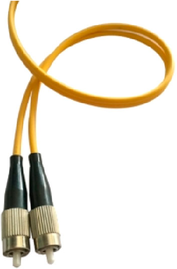
Figure 10. FC-type fiber optic connector.

Figure 11

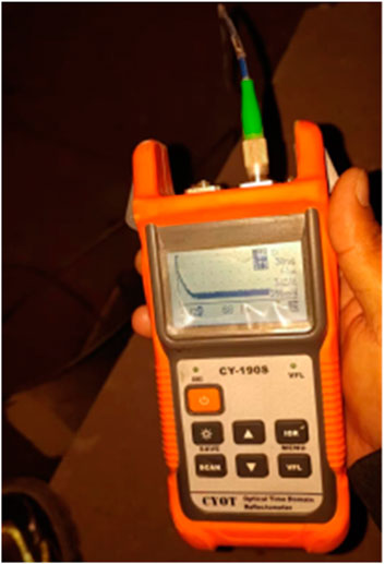
Figure 11. BOFDA demodulation unit.

Calculation of axial force and side friction

Axial forces were derived from the measured strains using the pile’s elastic modulus and cross-sectional area. The difference in axial force between two adjacent sections was then used to compute the side friction of the intervening soil layer, while the base force was divided by the pile toe area to obtain end resistance. The calculation formulas are as follows:

1. Axial force at pile section i

$N_i={\epsilon }_i·E_i·A_i,(1)$

where $N_i$ represents the axial force at section i of the pile (kN); ${\epsilon }_i$ represents the average axial strain at section i (dimensionless) (for long-term monitoring, creep effects should be eliminated); $E_{\mathrm{i}}$ represents the elastic modulus of the material at section i (kPa); and $A_i$ represents the cross-sectional area at section i (m²).

2. Layered side friction and end resistance

$\begin{array}{l}{q}_{si}=\frac{N_i-N_{i+1}}{u\times l_i}\\ q_p=\frac{N_p}{A_p}\end{array},(2)$

where $q_{si}$ represents the side resistance of the soil between sections i and i+1 (kPa); $q_p$ represents the end resistance (kPa); $i$ represents the index of pile measurement sections, numbered from top to bottom (i = 1, 2, …, n); $u$ represents the pile perimeter (m); $l_i$ represents the pile length between sections i and i+1 (m); $N_p$ represents the axial force at the pile base (kN); and $A_p$ represents the cross-sectional area at the pile base (m²).

Test data and results

Distributed axial strain profile

Distributed fiber optic data acquisition was carried out simultaneously with the staged loading and unloading of the static load tests. This work served as an auxiliary test, and the data are provided for reference. Pile parameters and acquisition stages are summarized in Table 8, and the collected data were used to construct strain–depth profiles (Figures 12–20).

Table 8

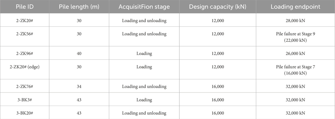
Table 8. Pile parameters and acquisition stages.

Figure 12

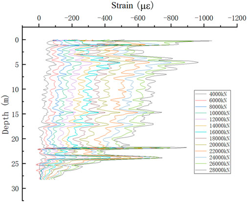
Figure 12. Strain distribution of pile 2-ZK20# during loading.

Figure 13

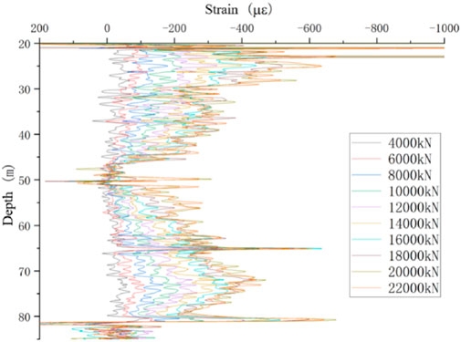
Figure 13. Strain distribution of pile 2-ZK56# during loading.

Figure 14

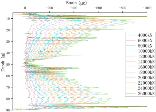
Figure 14. Strain distribution of pile 2-ZK96# during loading.

Figure 15

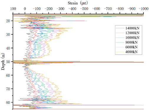
Figure 15. Strain distribution of pile 2-ZK20# (edge) during loading.

Figure 16

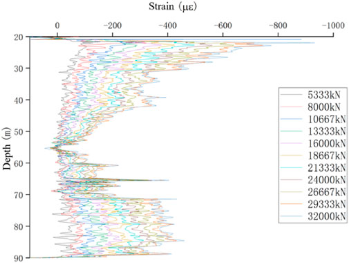
Figure 16. Strain distribution of pile 2-ZK76# during loading.

Figure 17

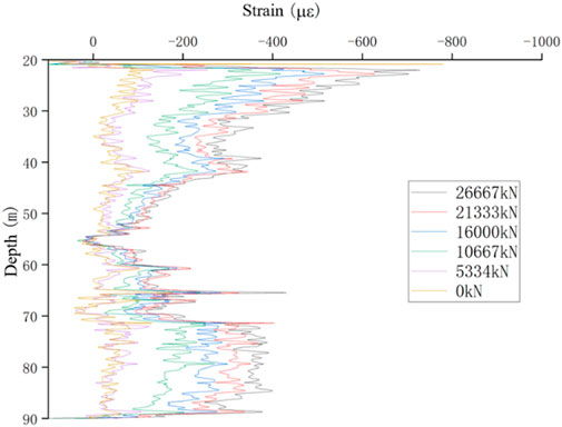
Figure 17. Strain distribution of pile 2-ZK76# during unloading.

Figure 18

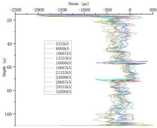
Figure 18. Strain distribution of pile 3-BK3# during loading.

Figure 19

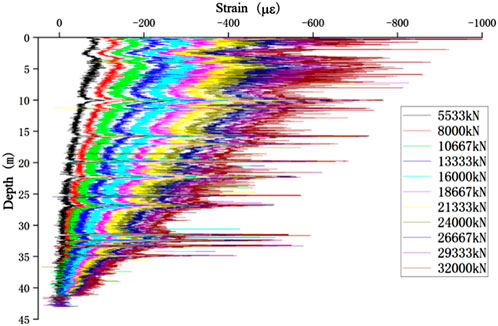
Figure 19. Strain distribution of pile 3-BK20# during loading.

Figure 20

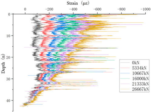
Figure 20. Strain distribution of pile 3-BK20# during unloading.

It should be noted that due to site limitations, piles 2-ZK96# and 2-ZK20# reached the maximum capacity of the testing apparatus; the test was ended prior to the standard requirement was met.

Pile 3-BK20# was selected as typical for further analysis. Rather than presenting the U-shaped fiber data, the raw measurements were processed through a preliminary filter and are presented as follows:

The main features of the acquired data are summarized as follows:

1. Synchronized acquisition: Fiber data were collected at each load stage after stabilization. Except for pile 3-BK20# (acquired at 0.01 m resolution), all piles were recorded at 0.05 m resolution. Each dataset contained no fewer than 2,000 points, with more than 1,000 effective data points, providing a clear representation of the pile shaft’s staged loading–unloading response.

2. Imperfect axis symmetry: With U-shaped cable layouts, strain data are theoretically symmetric about the pile bottom. In practice, bending of the fiber tied along the reinforcement bars caused discrepancies between the two sides, resulting in only a symmetric trend rather than perfect correspondence. Data processing, therefore, adopted either single-sided data or averaged values from both sides after separate fitting.

3. Data correction at the pile head: Fibers extended through the pile cap, recording strain in both the pile and the cap. As the cap concrete grade (C50) differed from that of the pile (C40), the recorded top strain did not represent the maximum load condition at the pile head. Corrections were therefore required to align the top strain with the applied load.

4. Positive strain values: In geotechnical convention, compressive strain is positive and tensile strain is negative. However, in fiber data acquisition, compressive strain appears as negative, and tensile strain appears as positive. Small curvatures caused by stirrups, splices, or grouting pipes introduced local tensile readings during loading/unloading. These isolated positive values may be removed or retained if they do not affect the overall strain trends.

5. Interference at cable ends: Fiber bridging with lead cables caused fluctuations at both ends of the dataset. Because these regions do not contribute to side friction analysis, the jump-line segments were excluded, retaining only valid pile shaft and pile cap strain data.

Along the entire pile, occasional negative values did occur, although no significant fluctuations were observed in the values of side friction. This phenomenon was caused by large deviations between adjacent strain points during the calculations. Because fiber optic measurements are highly sensitive and densely distributed, slight protrusions may occur at reinforcement joints where the fiber is tied, as shown in Figure 21. At these protrusions, the axial strain may be recorded as tensile rather than compressive, producing localized tensile strain readings, which can lead to invalid axial force calculations in the affected zone and cause unusual fluctuations in the collected data. To address this, manual adjustments were introduced during data processing as described earlier. Nevertheless, due to the harsh field conditions, fiber installation could not be as ideal as in laboratory settings and, thus, more manual intervention and correction were required.

Figure 21

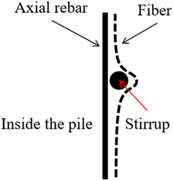
Figure 21. Schematic of fiber arrangement at the interaction of rebar.

Overall, the BOFDA measurements provided high-resolution strain profiles—typically with more than 2,000 points per pile—that captured both the general decay of strain with depth and the localized effects of soil variability and construction details. These profiles form the basis for the subsequent calculation of axial force and side friction distributions.

The side-distributed side friction profiles

Side friction (q_si) of the cast-in-place pile is calculated based on Equation 2 from the axial strain data collected. For engineering interpretation, the average value within each soil layer was taken as its representative side friction. An example is shown in Table 9 and Figure 22 for pile 3-BK20#, where side friction is presented for individual strata under different surcharge loadings.

Table 9

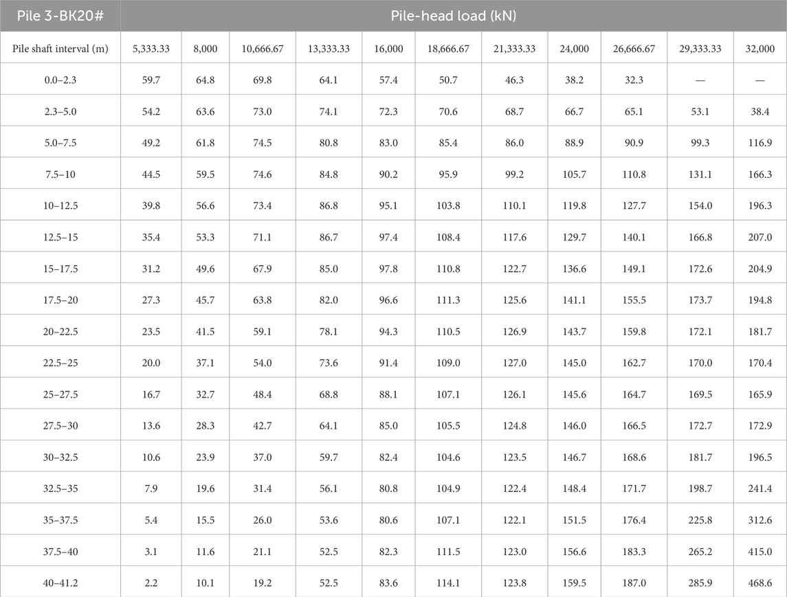
Table 9. Side friction resistance of pile 3-BK20# at different depth intervals under various load levels (kPa).

Figure 22

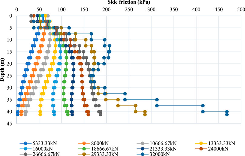
Figure 22. Side friction distribution of pile 3-BK20# under varying surcharge loads across soil layers.

Figure 22 shows that, at low load levels, the side friction near the pile head was well mobilized, gradually decreasing with depth and approaching zero near the pile toe. This distribution is consistent with the conventional understanding that friction piles initially resist load primarily through side friction in the upper strata. As the applied load increased, however, the side friction near the pile head increased sharply and, in some cases, decreased again once local sliding occurred. This transition from static to dynamic friction produced localized reductions in resistance, while deeper sections progressively mobilized additional side friction and, eventually, tip resistance.

Similarly, the results of other piles are presented as Figures 23–28. Although the general trend of “greater head load resulting in greater mobilization at depth” was observed in most piles, local irregularities were also evident. For example, in piles 2-ZK20# (edge) and 2-ZK20, the side friction distribution followed the same pattern identified in pile 3-BK20#, with tip resistance remaining low at small loads and increasing as the head load increased. In contrast, other piles exhibited more erratic distributions, with localized peaks and troughs appearing at different depths. These irregularities are attributed to variability in soil–pile contact conditions, such as the presence of boulders or changes in the degree of weathering.

Figure 23

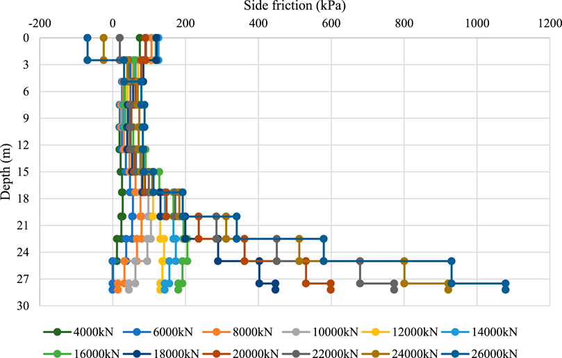
Figure 23. Side friction distribution of pile 2-ZK20.

Figure 24

Figure 24. Side friction distribution of pile 2-ZK56#.

Figure 25

Figure 25. Side friction distribution of pile 2-ZK96#.

Figure 26

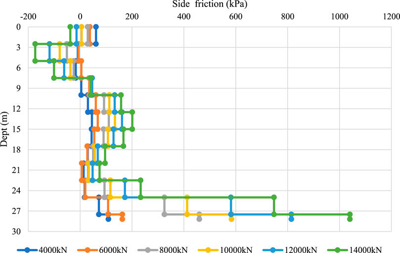
Figure 26. Side friction distribution of pile 2-ZK20# (edge).

Figure 27

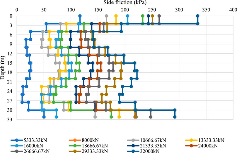
Figure 27. Side friction distribution of pile 2-ZK76#.

Figure 28

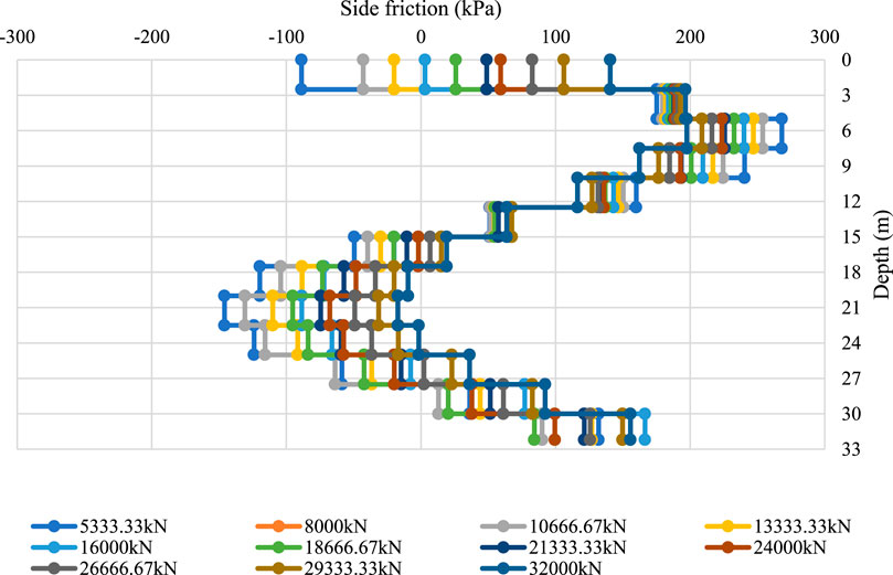
Figure 28. Side friction distribution of pile 3-BK3#.

In pile 2-ZK96#, the calculated side friction at the pile tip was exceptionally high. This anomaly is likely linked to fiber distortion at the pile end during installation, which, under load, caused the fiber to register exaggerated strains. Such distortion not only produced an unrealistically large tip resistance but also influenced the interpretation of strain data in the overlying sections.

Similarly, pile 3-BK3# showed poor data quality: while side friction appeared continuous with depth, numerous negative values were recorded, with the minimum occurring mid-pile. This distribution is inconsistent with expected load-transfer behavior and is most plausibly explained by an error in fiber installation at the middle segment, where tensile strains were erroneously measured instead of compressive strains. These cases underscore the difficulty of achieving ideal fiber placement under field conditions and the importance of rigorous data screening and correction.

In general, the distributed side friction profiles demonstrate both the advantages and challenges of BOFDA monitoring. On one hand, the technology captures progressive mobilization and identifies the onset of slippage, phenomena that conventional point-based instrumentation cannot resolve. On the other hand, its sensitivity makes the results vulnerable to local installation defects and soil variability, requiring careful interpretation. Despite these challenges, the profiles provide valuable insights into the transition of friction piles from side-resisting to tip-resisting behavior under high loads, offering a diagnostic capability that supports refined load-transfer modeling and more informed design practice.

Distributed side friction at different soil layers

The side friction is calculated along seven piles in the same area. It is possible to estimate the representative side friction value for different soil layers for further engineering purposes. For general purposes, the calculated average value for an individual soil layer is taken as the representative side friction of that soil, which is summarized in Table 10 and Figure 29.

Table 10

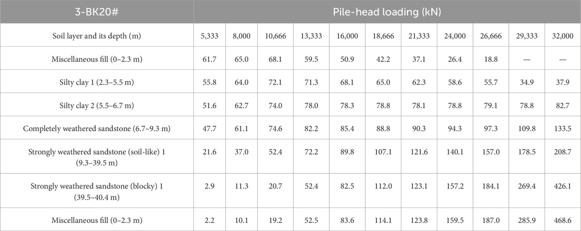
Table 10. Side friction distribution of pile 3-BK20# in different soil layers under different levels of surcharge loading.

Figure 29

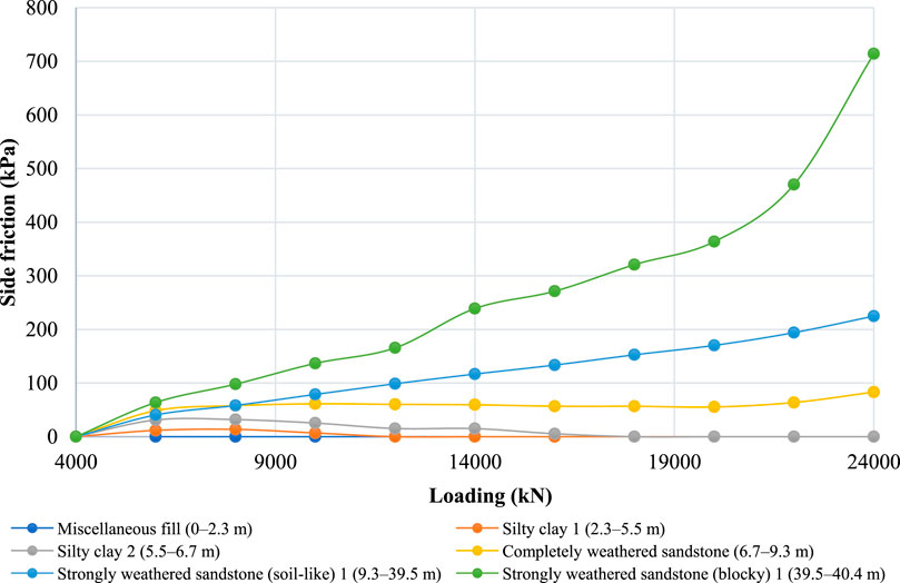
Figure 29. Side friction distribution of pile 3-BK20# in different soil layers under different levels of surcharge loading.

Figure 29 presents the side friction mobilization with increased surcharge loading. In general, side friction in the deep layer carried the greater part of the total resistance and gradually decreased along the pile length.

Meanwhile, under loading at approximately 9,000 kN, the upper soil layer of miscellaneous fill and silty clay shows a relatively higher capacity than it does at higher loading levels. However, when the applied loading exceeds the capacity of such layers, friction begins to reduce, which indicates that relative movement has occurred and, thus, no friction is calculated.

Deeper layers, such as completely decomposed granite (CDG) and weathered sandstone, are gradually mobilized and compensate for the capacity loss of the upper layer. It can be concluded that when designing a side-friction pile, any relative movement that could significantly reduce side friction should be carefully considered.

The remaining results are presented in Figures 30–35.

Figure 30

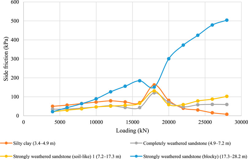
Figure 30. Side friction distribution of pile 2-ZK20# across different soil layers under different surcharge loads.

Figure 31

Figure 31. Side friction distribution of pile 2-ZK56# across different soil layers under different surcharge loads.

Figure 32

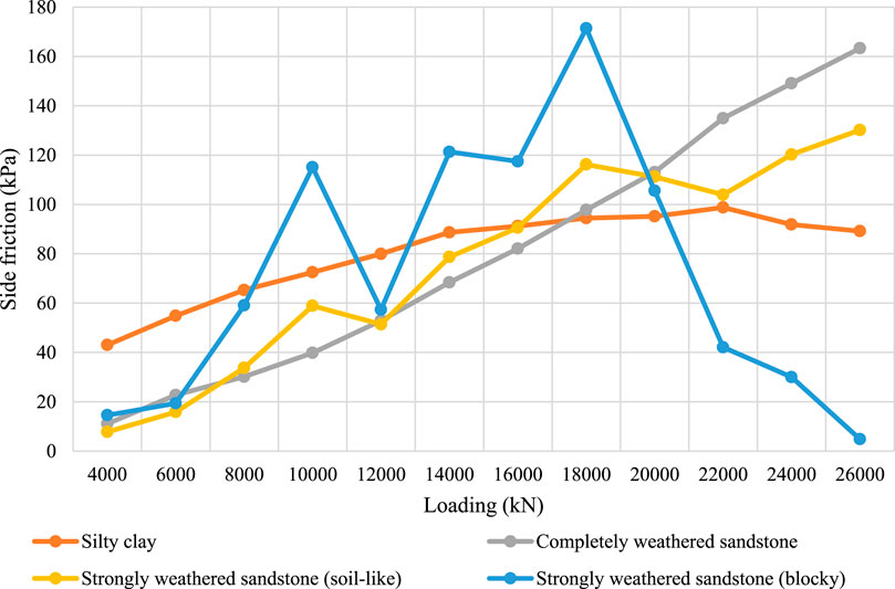
Figure 32. Side friction distribution of pile 2-ZK96# across different soil layers under different surcharge loads.

Figure 33

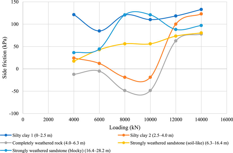
Figure 33. Side friction distribution of pile 2-ZK20# (edge) across different soil layers under different surcharge loads.

Figure 34

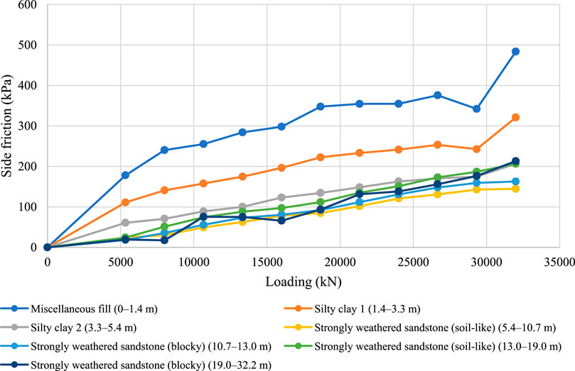
Figure 34. Side friction distribution of pile 2-ZK76# across different soil layers under different surcharge loads.

Figure 35

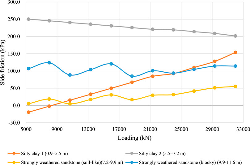
Figure 35. Side friction distribution of pile 3-BK3# across different soil layers under different surcharge loads.

Discussion

Comparison of the BOFDA-derived side friction with the site investigation (SI) recommendations shows that the measured values are generally lower, confirming the conservative nature of design practice. Such conservatism is appropriate for ensuring safety, but it may also prevent the full mobilization of pile capacity, particularly in friction piles where side friction governs performance.

The distributed strain data reveal details of load transfer that extend beyond the assumptions of conventional t–z models. In theory, side friction increases progressively with depth as lateral pressure and interface friction develop. The BOFDA profiles show that this pattern persists at lower loads, with resistance concentrated near the pile head and diminishing toward the toe. With increasing load, however, two departures from the idealized distribution were observed. First, in several piles, local peaks of resistance were recorded in zones where pile–soil contact was enhanced by boulders or denser strata, while resistance below these zones was weakened. This suggests that local geology governs the sequence of friction mobilization along the shaft. Second, at higher load levels, a sharp reduction in resistance near the pile head was observed, indicating the onset of relative sliding. Once static friction was exceeded, the interface transitioned to dynamic friction, reducing capacity locally and shifting more load transfer to deeper sections and the pile tip.

The statistics in Table 11 support these interpretations. In silty clay layers, BOFDA results ranged from 10 kPa to 80 kPa, mostly below the SI recommendation of 20 kPa. In completely weathered sandstone, measured values were typically 30 kPa–80 kPa compared with the recommended 50 kPa. In strongly weathered sandstone, results were more variable: many fell within the expected range (80 kPa–110 kPa), but some piles produced unusually high readings, up to 400 kPa. These anomalies likely stem from fiber irregularities at reinforcement ties or local soil–pile conditions, which produced exaggerated strain responses. Such variability highlights both the sensitivity of distributed sensing and the challenges of achieving uniform fiber installation in the field.

Table 11

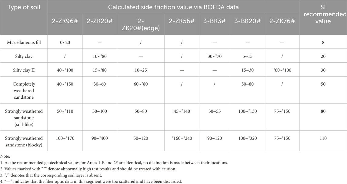
Table 11. Summary of calculated side friction vs. SI recommended values.

Taken together, the results demonstrate that the mobilization of side friction is controlled by both stratigraphy and the loading path. Under moderate loading, piles behave predominantly as side-resisting elements. Under higher loads, however, sliding near the pile head and progressive mobilization at depth cause a shift toward tip resistance. This transition, which is difficult to detect with conventional point sensors, was clearly captured by BOFDA. The findings underscore the potential of distributed sensing to provide not only validation of conservative design values but also detailed insights into the mechanics of pile–soil interaction that can inform more refined analysis and improved construction practice.

Conclusion

BOFDA was applied to monitor seven cast-in-place piles, yielding continuous strain profiles for axial force and side friction calculations. The results show that measured side frictions were generally lower than the recommended values from site investigation, confirming the conservative nature of current design practice. At the same time, the distributed measurements revealed localized anomalies: high resistances at boulder contacts or in weathered sandstone layers and premature sliding near the pile head under increasing loads. These observations indicate that side friction mobilization is strongly influenced by soil variability and interface conditions and that friction piles under heavy loading may progressively transition toward tip resistance.

The findings highlight the value of BOFDA in capturing load-transfer behavior that cannot be resolved with conventional instrumentation. Beyond validating the safety of conservative design, distributed sensing offers detailed diagnostic data that can support refinement of t–z models, improve construction quality control, and provide a basis for more efficient use of pile capacity in practice.

Data availability statement

The datasets presented in this article are not readily available because the dataset supporting this study was obtained from field pile load tests conducted within a construction project and contains proprietary engineering data. Due to confidentiality agreements with the project stakeholders, the raw data are not publicly available. Processed data relevant to the findings are available from the corresponding author upon reasonable request. Requests to access the datasets should be directed toeWNoZW5fOTEwOUBvdXRsb29rLmNvbQ==.

Author contributions

YC: Formal analysis, Funding acquisition, Investigation, Methodology, Software, Supervision, Writing – original draft, Writing – review and editing, Conceptualization. Z-GT: Data curation, Resources, Supervision, Writing – review and editing. M-LH: Data curation, Formal Analysis, Software, Validation, Visualization, Writing – original draft. Y-LG: Data curation, Project administration, Supervision, Writing – review and editing. Y-JW: Data curation, Investigation, Methodology, Writing – review and editing. G-HY: Funding acquisition, Investigation, Project administration, Resources, Writing – review and editing.

Funding

The author(s) declare that financial support was received for the research and/or publication of this article. The National Key Research and Development Program of China (grant no. 2022YFC3800901) provided financial support for the experimental design, data collection, and analysis phases of the project.

Conflict of interest

Authors YC, M-LH, Y-LG, Y-JW, and G-HY were employed by the company Central Research Institute of Building and Construction Co., Ltd., MCC Group.

Author Z-GT was employed by Shenzhen Geotechnical Engineering Co., Ltd.

Generative AI statement

The author(s) declare that no Generative AI was used in the creation of this manuscript.

Any alternative text (alt text) provided alongside figures in this article has been generated by Frontiers with the support of artificial intelligence and reasonable efforts have been made to ensure accuracy, including review by the authors wherever possible. If you identify any issues, please contact us.

Publisher’s note

All claims expressed in this article are solely those of the authors and do not necessarily represent those of their affiliated organizations, or those of the publisher, the editors and the reviewers. Any product that may be evaluated in this article, or claim that may be made by its manufacturer, is not guaranteed or endorsed by the publisher.

References

Bado, M. F., and Casas, J. R. (2021). A review of recent distributed optical fiber sensors applications for civil engineering structural health monitoring. Sensors 21 (5), 1818–1883. doi:10.3390/s21051818

PubMed Abstract | CrossRef Full Text | Google Scholar

Bernini, R., Minardo, A., and Zeni, L. (2012). Distributed sensing at centimeter-scale spatial resolution by BOFDA: measurements and signal processing. IEEE Photonics J. 4 (1), 48–56. doi:10.1109/JPHOT.2011.2179024

CrossRef Full Text | Google Scholar

Ding, Y., Wang, P., Li, P. F., Xia, T., and Tang, J. L. (2014). Monitoring technology of deformation of continuous concrete wall based on BOTDA. Yantu Gongcheng Xuebao/Chinese J. Geotechnical Eng. 36, 500–503. doi:10.11779/CJGE2014S2087

CrossRef Full Text | Google Scholar

Fu, C., Peng, Z., Li, P., Meng, Y., Zhong, H., Du, C., et al. (2023). Research on distributed fiber temperature/strain/shape sensing based on OFDR. Laser Optoelectron. Prog. 60 (11), 1106007. doi:10.3788/LOP230701

CrossRef Full Text | Google Scholar

Garus, D., Gogolla, T., Krebber, K., and Schliep, F. (1996). Distributed sensing technique based on brillouin optical-fiber frequency-domain analysis. Opt. Lett. 21 (17), 1402. doi:10.1364/ol.21.001402

PubMed Abstract | CrossRef Full Text | Google Scholar

Guo, Z., and Zhao, Z. (2018). Application of distributed optical fiber sensing technique in pile foundation monitoring. IOP Conf. Ser. Earth Environ. Sci. 189 (5), 052074. doi:10.1088/1755-1315/189/5/052074

CrossRef Full Text | Google Scholar

Lu, P., Lalam, N., Badar, M., Liu, Bo, Chorpening, B. T., Buric, M. P., et al. (2019). Distributed optical fiber sensing: review and perspective. Appl. Phys. Rev. 6 (4), 041302. doi:10.1063/1.5113955

CrossRef Full Text | Google Scholar

Ma, J., Pei, H., Zhu, H., Shi, B., and Yin, J. (2023). A review of previous studies on the applications of fiber optic sensing technologies in geotechnical monitoring. Rock Mech. Bull. 2 (1), 100021. doi:10.1016/j.rockmb.2022.100021

CrossRef Full Text | Google Scholar

Minardo, A., Catalano, E., Coscetta, A., Zeni, G., Zhang, L., Di Maio, C., et al. (2018). Distributed fiber optic sensors for the monitoring of a tunnel crossing a landslide. Remote Sens. 10 (8), 1291. doi:10.3390/rs10081291

CrossRef Full Text | Google Scholar

Minardo, A., Zeni, L., Coscetta, A., Catalano, E., Zeni, G., Damiano, E., et al. (2021). Distributed optical fiber sensor applications in geotechnical monitoring. Sensors 21 (22), 7514. doi:10.3390/s21227514

PubMed Abstract | CrossRef Full Text | Google Scholar

New York Climate Week (2024). Addressing the $94 trillion infrastructure investment gap. Available online at: https://www.fastinfralabel.org/news/new-york-climate-week-2024-addressing-the-94-trillion-infrastructure-investment-gap.2024.

Google Scholar

Schenato, L., Palmieri, L., Camporese, M., Bersan, S., Cola, S., Pasuto, A., et al. (2017). Distributed optical fibre sensing for early detection of shallow landslides triggering. Sci. Rep. 7 (1), 14686. doi:10.1038/s41598-017-12610-1

PubMed Abstract | CrossRef Full Text | Google Scholar

Wu, R., Biondi, A., Cao, L., Gandhi, H., Abedin, S., Cui, G., et al. (2023). Composite bridge girders structure health monitoring based on the distributed fiber sensing textile. Sensors 23 (10), 4856. doi:10.3390/s23104856

PubMed Abstract | CrossRef Full Text | Google Scholar