Exploring the spatial variation of intra-urban housing prices based on inverse S-function fitting of 35 cities

Housing prices serve as a crucial indicator of macroeconomic stability and urban spatial vitality. However, existing studies on intra-urban housing prices predominantly focus on single-city empirical analyses or localized examinations of individual factors, often lacking holistic approaches and cross-city comparative perspectives. Given the widespread application of the inverse S-function and its suitability for characterizing the spatial distribution of housing prices, this study employs this function to model the spatial variation of housing prices across 35 major Chinese cities. Methodologically, we identify urban centers through kernel density estimation and apply circle-layer gradient analysis to establish price gradients. Building on this foundation, we fit the inverse S-function model and further develop two quantitative indices—stability and concentration—for in-depth analysis. The results reveal that all 35 cities exhibit significant spatial agglomeration of housing prices according to global Moran’s I analysis. The inverse S-function achieves an average R² of 0.98 in fitting price decay, categorizing the curves into three types: standard inverse S-decay, fast-then-slow decay, and linear decay. The two indices further indicate that cities with higher levels of economic development (e.g., Beijing, Shanghai) exhibit stronger spatial aggregation and stability in housing prices. In contrast, cities in the western and northeastern regions (e.g., Xining, Hohhot) demonstrate a significantly faster rate of price decline from the urban center outward. This study provides a new quantitative method for research on the spatial distribution of intra-urban housing prices and offers a reference for urban planning and real estate regulation policies.

1 Introduction

Residential property prices serve as a pivotal barometer of both macroeconomic stability and urban spatial vitality, embodying the intricate interplay between market dynamics, policy interventions, and societal needs. Internationally, real estate markets have long been recognized as deeply intertwined with national economic cycles—with historical crises from the U.S. subprime mortgage collapse to Japan’s “lost decades” underscoring how housing price volatility can amplify systemic risks (Reinhart and Rogoff, 2009). Beyond economic implications, housing prices function as a critical indicator of urban resource allocation: they reflect the accessibility of core public services, the attractiveness of neighborhoods, and the distribution of socio-economic opportunities across city spaces (Cheshire and Sheppard, 2002). The spatial differentiation of housing prices directly links regional economic vitality to resident wellbeing and quality of life. Consequently, researching the spatial patterns of housing prices is essential for formulating equitable urban development strategies and enhancing overall societal wellbeing. Due to the differences in various aspects such as economy, population, and public services, there are also significant differences in the level of intra-urban housing prices in different regions. Since exploring the spatial distribution of intra-urban housing prices is helpful to understand the level of real estate development in each region of the urban, and then to formulate reasonable urban planning and real estate regulation policies, the spatial distribution of urban property prices has become one of the hot issues of interest to urban geographers.

Scholars have conducted research on the spatial distribution of housing prices in different cities, especially with the help of GIS spatial analysis methods in recent years, and a series of research results have been achieved (Chen, 2018; Wang and Yang, 2024; Kenyon et al., 2024). Scholars have also explored the influencing factors of urban housing prices from multiple dimensions, such as urban spatial form, public transportation systems, and commercial shopping centers (Aliyar et al., 2023; Fandian and Panwar, 2025; Yoğurtçu, 2024). However, existing research still exhibits significant limitations: most studies focus on empirical analyses of single cities, with descriptions of the spatial distribution of housing prices being predominantly qualitative, lacking sufficient quantitative analysis, and there is a scarcity of cross-city comparative studies. More importantly, much of the existing research concentrates on exploring the local effects of single influencing factors, while neglecting the systematic investigation of the overall distribution patterns of housing prices in urban space.

Urban spatial structure is the manifestation of the distribution and combined relationships among the material, economic, functional and cultural components in a city (Wang et al., 2014). The traditional patterns of urban spatial structure include the concentric circle pattern proposed by Burgess in 1925, the fan pattern proposed by Hoyt in 1939, and the multi-core pattern proposed by Harris and Ullman in 1945 (Niu, 2008). From the perspective of economics, the urban spatial structure is mainly the urban land use structure based on the land rent theory. According to the location selection rules of different economic actors, a concentric-circle-like land use pattern is formed based on differences in bid rents, which also constitutes the fundamental logic of urban spatial structure evolution (Feng and Zhou, 2003). Urban housing prices also show a similar distribution pattern of concentric circles spatially: the value of land resources is highest in the urban center and gradually decreases outward along a uniform radius. The core reason lies in the centripetal force formed by the concentration of various resources in the city center, which influences the distribution of housing prices, resulting in a concentric-circle structure in the spatial pattern. Previous studies have also confirmed similar rules (Manzoli and Mocetti, 2019; Laziou et al., 2025). For example, Wang et al. (2022) found that housing prices in the study area of Wuhan gradually increased from the urban fringe area to the urban core area and its surroundings, and the housing prices showed a gradual downward trend from the city center to the periphery in the horizontal direction. So, is this circle structure common in cities? Is the decline trend homogeneous across circles? Is it possible to describe this decreasing pattern by a specific function?

Scholars have employed various functional forms, such as inverse power functions, exponential functions, and Gaussian models, to fit and analyze the spatial evolution characteristics of urban elements, including built-up area density, population density, and POI distribution density (Batty and Kim, 1992; Xu et al., 2019b; Yang et al., 2022; Gui et al., 2024). Among them, Jiao (2015) proposed an urban land density function in 2015, which quantitatively portrayed the spatial attenuation pattern of urban land density from the urban center to the periphery using the inverse S-function, and this model has been widely applied to measure the spatial distribution of other elements in cities (Xu et al., 2019a; Li et al., 2021; Zheng et al., 2023). Compared to other function models, the inverse S-function more accurately captures the three-stage characteristic of “gentle stability in the core area - rapid decay in the transition area - gradual stabilization in the peripheral area,” making it better suited to describe the spatial variation pattern of urban housing prices. Therefore, we try to quantitatively fit the distribution of urban housing prices by using inverse S-function.

To sum up, this study divides the cities into circles with concentric circles, and calculates the average value of the housing prices within each circle, based on the housing price data of commercial residential communities (residential communities for short) within 35 cities. On this basis, we use inverse S-function to fit, trying to accurately describe the decaying law of urban housing prices from the urban center to the surrounding areas. The parameters of the function can assist in understanding the distribution pattern of urban housing prices. The results of this study are conducive to a deeper understanding of the distribution pattern of intra-urban housing prices, and provide support for relevant urban planning decisions.

To this end, the study was structured in five stages. First, it elaborated on the research background, significance and status of intra-urban housing price spatial variation. Second, it detailed data sources and processing methods. Third, it introduced specific research methods: kernel density estimation for urban center identification and monocentric/polycentric classification, circle-layer gradient analysis for dividing residential communities into layers and calculating average housing prices, and the principle and form of the inverse S-function for housing price fitting. Fourth, it presented the results, covering the inverse S-function’s fitting effect, types of housing price decay curves, calculation results of the housing price stability and concentration indices, and cross-city comparative analysis of housing price spatial patterns. Finally, it summarized the main conclusions, and discussed the theoretical contribution and practical significance.

2 Materials/data and processing

This study analyzes the spatial distribution of housing prices across 35 major Chinese cities, a sample selected to ensure national representativeness, socioeconomic diversity, and data consistency. The sample encompasses four municipalities directly under the central government, 26 provincial capitals (excluding Taipei), and five cities specifically designated in the state plan. These cities constitute the upper echelon of China’s urban system, characterized by their significant population size, economic influence, and mature housing markets with pronounced spatial differentiation. Geographically, they cover China’s four major regions (eastern, central, western, and northeastern) and include diverse city types, which supports the generalizability of our findings.

Within this analytical framework, the residential community serves as the fundamental data unit, as it constitutes the basic building block of urban residential areas in China, and community-level price data are widely accessible. Housing price data for residential communities were sourced from Soufun, China’s leading and largest online real estate platform (Zhang and Wang, 2025). Using a customized web crawler, we collected location data (latitude and longitude) and housing price data for residential communities across 35 major Chinese cities. To ensure temporal consistency, all housing prices reflect market values as of August 2020. Taking Beijing as an example, the data collection process proceeded as follows: after accessing the Soufun homepage and setting the target city to Beijing, we selected the “residential communities” module to retrieve the complete listing of over 20,000 communities in the city. For each community, we systematically extracted its name, housing price, spatial coordinates, community type, construction year, and other relevant attributes. The same standardized methodology was consistently applied across all 35 cities to compile the comprehensive dataset of raw community-level housing prices.

Ensuring data quality is essential for the reliability of our conclusions; therefore, we implemented a rigorous data-cleaning process. Using Beijing as an example, this process consisted of three steps: First, missing values were addressed by removing records with incomplete data for critical variables such as housing prices and spatial coordinates. For non-critical variables like community type or construction year, missing entries were temporarily labeled as “unknown,” and additional searches were conducted to supplement information where possible. Second, data filtering was conducted to exclude non-standard residential communities (e.g., villa compounds) and those over 40 years old to ensure sample comparability. Third, outliers were identified and removed using statistical methods: after the above filtering, the 1st and 99th percentiles of community-level housing prices were calculated, and values outside this range were excluded. Robustness checks were also performed using alternative thresholds (99.5th and 95th percentiles).

Additionally, points of interest (POIs) for urban commercial facilities across all 35 cities were collected using Baidu Map API for the identification of urban center points.

3 Implementation process

The steps of function fitting are as follows: 1) analyzing the spatial clustering of urban housing prices using spatial autocorrelation; 2) identifying each urban center using the kernel density function; 3) dividing circles outward from each urban center and counting the mean housing price within each circle; 4) fitting with the inverse S-function.

3.1 Spatial autocorrelation

To initially explore the spatial distribution pattern of intra-urban housing prices, we first conduct a qualitative analysis to measure whether there is a spatial agglomeration phenomenon, that is, spatial autocorrelation. Global Moran’s I index is calculated for housing prices of residential communities in all cities. The results are shown in Table 1.

Table 1

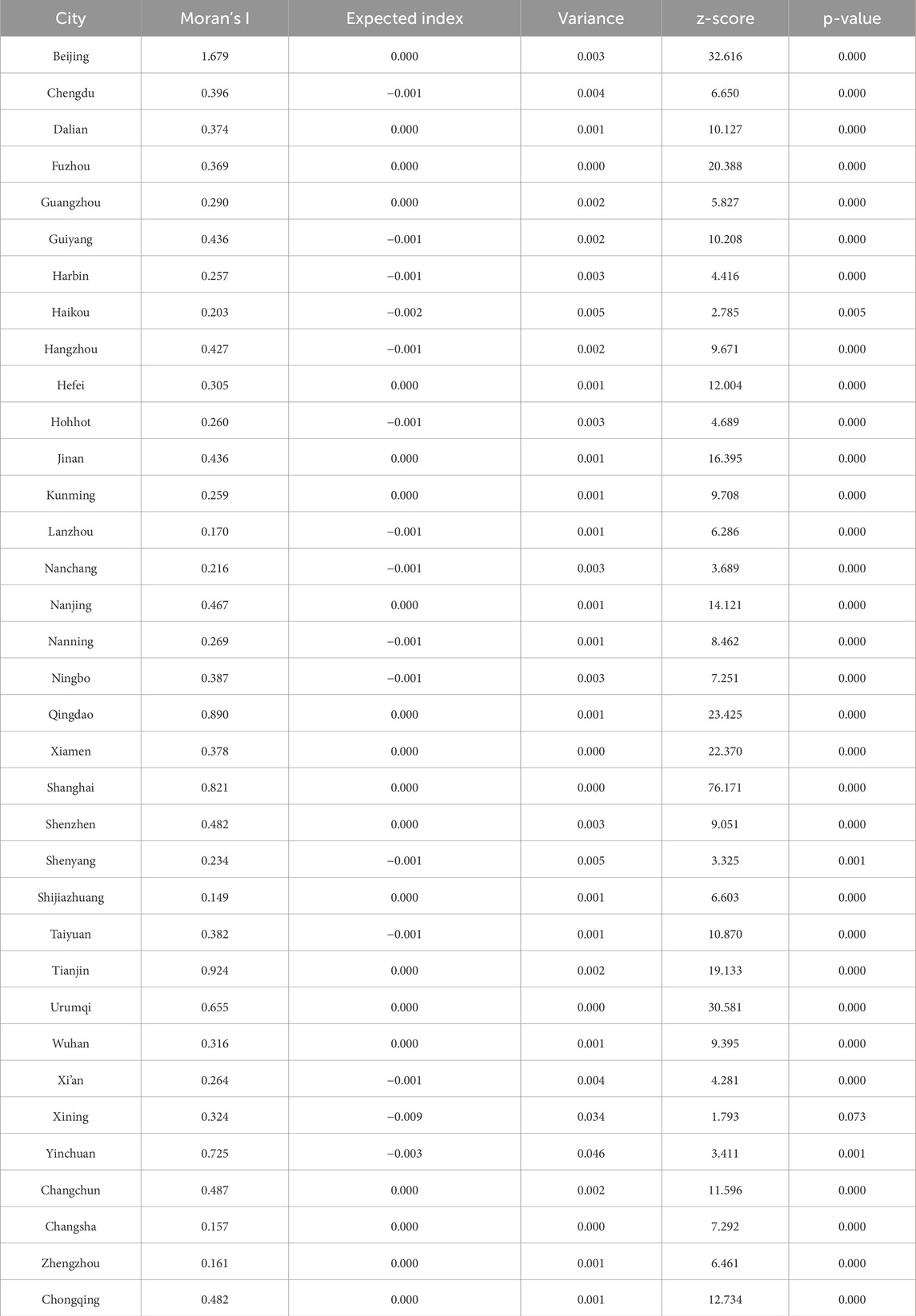
Table 1. Global Moran’s I index of housing prices in residential communities.

Table 1 shows that the spatial autocorrelation of the selected sample of 35 cities is greater than 0, with a statistically significant p-value. This indicates that housing prices in all cities exhibit varying degrees of spatial autocorrelation, i.e., a spatial agglomeration phenomenon. Subsequently, we adopt the function fitting method to quantitatively analyze the spatial distribution pattern of housing prices.

3.2 Urban center identification

Kernel density estimation (KDE) is used to estimate unknown density functions in probability theory, as one of the non-parametric testing methods (Yu et al., 2016). In the field of GIS, kernel density analysis tools are used to calculate the density of elements such as points and lines in their surrounding neighborhoods (Elgammal et al., 2002; Borruso, 2008). For example, it is used to measure building density, to obtain crime reports, and to identify road or utility lines that impact towns or wildlife habitat. With the development of web technology and the rise of big data technology, scholars have used POI data, social media data, and mobile phone signaling data to identify urban centers and other urban functional areas (Leslie, 2010; Veneri, 2013; Sun et al., 2016; Song et al., 2020). For example, Yu et al. (2015) took Shenzhen and Guangzhou as examples, and used the kernel density estimation method based on path distance to identify urban centers. It can be expressed with the Equation 1.

$\mathrm{f}\left(\mathrm{x}\right)=\frac{1}{nh}{\displaystyle \sum _{i=1}^n}K\left(\frac{x-x_i}{h}\right)(1)$

Where f(x) is the estimated value of kernel density at the spatial position x; h is the distance attenuation threshold, i.e., bandwidth; k is the spatial weight function; n is the number of elements whose distance from x is less than h; and $x-x_i$ is the distance between the estimated point x and neighboring points.

To simplify the calculation, this study uses the kernel density estimation method combined with urban zoning and planning to determine the urban center points of the 35 target cities. Due to the differences in the economic level, natural conditions, historical evolution and development strategies of cities, the location and number of urban centers are different. According to the identification results, the urban samples are classified into two categories: monocentric cities and polycentric cities. Among them, there are 20 monocentric cities, such as Fuzhou and Guiyang, and 15 polycentric cities, such as Xiamen and Lanzhou. The classification results are shown in Table 2.

Table 2

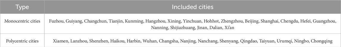
Table 2. Identification results of urban centers.

Figure 1 presents the results of POI kernel density and the selection of urban centers. Among them, Hangzhou is used as an example of a monocentric city, and Wuhan is used as an example of a polycentric city.

Figure 1

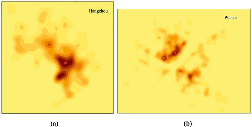
Figure 1. Identification of urban centers by kernel density. (a) monocentric city (b) polycentric city.

3.3 Circle-layer division

Circle-layer analysis is to first make a series of equidistant buffer zones outward with the urban center as the circle center, and the formed multi-ring buffers are used as the basic unit to describe the spatial differentiation of urban elements. Then, the density of relevant elements or the size of relevant attribute values in each unit can be counted (Li et al., 2003; Jiao and Dong, 2018). The circle-layer gradient analysis is used to classify the residential communities of each city into circles.

In the buffer analysis of the circle-layer method, the outermost buffer ring identifies the urban boundary, which should be large enough to include all target elements in theory. For monocentric cities, the points of residential communities are divided by making continuous buffer zones with an interval of 1 km outward from the urban center. For polycentric cities, according to the balanced polycentric hypothesis (i.e., multiple centers of the city are considered to be functionally equivalent and there is no differentiation between primary and secondary), multi-ring buffers with an interval of 1 km are made from different centers outward respectively, and the overlapping parts are fused. For the treatment of overlapping buffer zones, this study determines the final boundaries by applying a hierarchy-based priority rule during the buffer merging process. Considering that there will be errors in statistical results due to too few sample points within the circles in urban fringe areas, the boundary of the buffer zone (the outermost circle), used for subsequent housing price statistics, is set to be a circle containing at least 10 sample points of residential communities. Figure 2 shows the multi-ring buffer zone division for monocentric and polycentric cities, respectively, taking Hangzhou and Wuhan as examples.

Figure 2

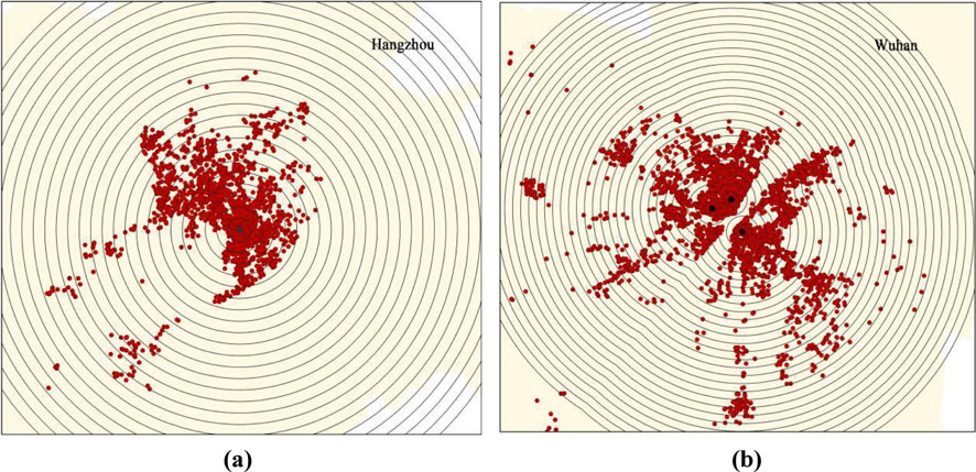
Figure 2. Circle-layer division results of residential communities. (a) monocentric buffer zone division (b) polycentric buffer zone division.

Next, we calculate the average value of the housing prices within each circle. The average housing price in the residential community falling in each circle is calculated according to the Equation 2.

$P_i=\frac{{\sum }_1^n{p}_j}{n}(2)$

Where is the average value of the housing prices in the ith circle; is the housing price of the jth residential community in the jth circle; j ranges from one to n; and n is the number of residential communities in the ith circle.

Since the housing prices of different cities are different in magnitude, in order to facilitate the horizontal comparison of the fitted function parameters, the circle-layer housing prices of each city after statistics, namely, the dependent variable y value, are normalized. The transformation formula is as follows (Equation 3):

$y^{\prime }=\frac{y}{y_{\mathit{max}}}(3)$

Where y is the average value of the housing price in the ith circle; is the highest housing price in the circle, which usually is the housing price in the first circle, i.e., the housing price in the urban center. The normalized housing price for each circle ranges from 0 to 1, representing the ratio of housing prices in a particular circle to those in the urban center.

3.4 Inverse S-function fitting

The inverse S-function can be used to describe the distribution pattern of geographic elements that exhibit an inverse S-shaped variation (Zheng et al., 2023). It was first applied to depict urban land density, which is highest at the city center, decreases rapidly from the inner city to the suburbs, and finally declines slowly at the urban periphery (Jiao, 2015). Urban elements generally display spatial agglomeration and similar distribution patterns. Therefore, besides urban land density, other geographic elements also tend to follow an “inverse S-shaped” pattern (Govind and Ramesh, 2020; Gao et al., 2025). Scatter plots of average housing prices across different urban zones reveal that prices roughly decrease in an inverse S-shaped manner from the city center outward. Accordingly, this study applies the inverse S-function to model the decay of urban housing prices from the center to the periphery. The original functional form is as follows (Equation 4):

$\mathrm{f}\left(\mathrm{r}\right)=\frac{1-c}{{1+e}^{\alpha \left(\left(\frac{2r}{D}\right)-1\right)}}+c(4)$

Where f(r) is the urban land density; r is the distance from the urban center; e is the Euler’s number; α, c and D are the fitting parameters, where α is the parameter controlling the slope of the urban density equation curve, c is the land density near the urban boundary, and D is the estimation result of the radius of the main urban area. Figure 3 shows the curve of urban land density function (inverse S-function), when α = 4, c = 0.05, D = 30.

Figure 3

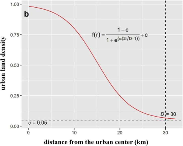
Figure 3. Schematic diagram of the inverse S-function curve.

The fitting process of this study was implemented in MATLAB R2020b, and Table 3 presents the resulting model parameters. R² reflects the fitting degree of the function to the data, and the results in the table show that the average fitting degree of the function is 0.98, indicating that the inverse S-function can well fit the spatial variation of housing prices in 35 cities in China. The function parameters α, c, and D have certain physical significance, representing some basic characteristics of the urban housing price distribution. Where α is the slope of the curve, representing the speed at which the housing price changes with distance. A larger value of α indicates that housing prices fall rapidly when the distance from the urban center increases. c is the asymptote of the function, indicating the limit value to which the housing prices can fall when it is far enough from the urban center, called the “limit housing price”. Since the housing price data is standardized, c represents the ratio of the limit housing price to the housing prices in the urban center here. From the fitting results, the value of c ranges from 0.22 to 0.68, indicating that there are large differences in the variation range of housing prices in different cities. According to the inverse S-equation, when r = D, the value of $f\left(D\right)=\frac{1-C}{1+e^{\alpha }}+is$ slightly greater than c, so D represents the distance from the urban center when the housing price drops to the limit value. For monocentric cities, D can be approximated as the limit of the urban edge (Jiao, 2015; Xu et al., 2019a).

Table 3

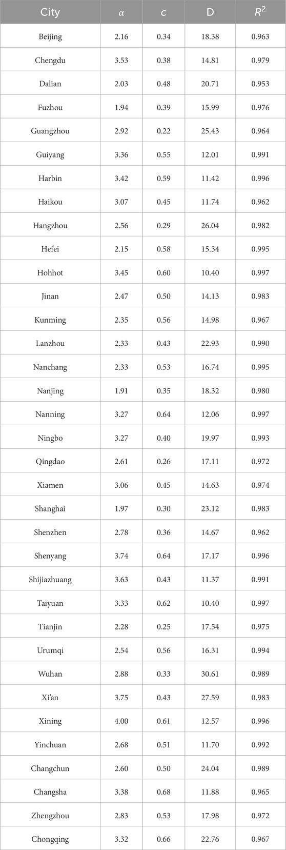
Table 3. Fitting results of housing price variation functions in residential communities.

4 Results

4.1 Spatial variation of urban housing prices

Based on the fitting results of the inverse S-function, the housing price curves for 35 cities were plotted (Figure 4). Results show that there are differences in the curves of housing prices with distance across different cities. Specifically, the change curves of housing prices in cities such as Chengdu, Haikou and Nanning are standard inverse S-shapes, with the change process containing three stages: a slow decline in housing prices in the central region, then a rapid decline, and finally a resumption of slow decline until reaching the limit housing price. The change curves of housing prices in cities such as Beijing, Harbin and Jinan contain two stages: a rapid decline in the near-center area, and a slow decline after a certain distance until reaching the limit housing price. However, the slopes of the housing price change curves in cities such as Lanzhou and Changchun are relatively small, showing a linear decay pattern from the urban center to the outside.

Figure 4

Figure 4. Inverse S-function fitting results of housing prices.

4.2 Measurement of housing price distribution form

The inverse S-function can not only fit the spatial variation of urban housing prices well, but also can characterize the distribution of urban housing prices to a certain extent through its fitted parameters.

4.2.1 Housing price stability index

The inverse S-shaped curve is characterized by a changing decay rate of the housing prices as distance increases. To further explore the characteristics of the curve, we attempt to solve the first and second derivatives of the function respectively. Specifically, the first derivative represents the declining rate of housing prices, and its extreme point is the point with the fastest declining rate, corresponding to the distance $r_0$, $r_0=$ The second derivative represents the rate of change of the decay rate, with its two extreme points indicating the locations where the change in the decay rate is greatest, corresponding to distances r₁ and r₂, as shown in Figure 5.

Figure 5

Figure 5. Calculation results of housing price stability index.

Therefore, the area from r₁ to r₂ can be regarded as the area with the fastest decline in housing prices in the whole city, and the scope of this area can reflect the spatial stationarity of housing prices to a certain extent (Angel et al., 2010). Cities with low housing price stationarity have higher prices in the core area, which then fall rapidly to the peripheral level. In contrast, those with high stationarity have a more gradual price decline from the center outward. However, the size of the range from r₁ to r₂, i.e., the value of $r_2-r_1$ is closely related to the urban scale, which may cause bias when comparing different cities. Therefore, the stability index of urban housing prices is defined as the proportion of the most rapidly declining areas of housing prices in the total urban area, calculated with Equation 5.

$\text{Sta}=\frac{r_2-r_1}{D}=\frac{1.316957}{\alpha }(5)$

Here, Sta represents the urban housing price stability index. A smaller Sta value indicates a smaller proportion of fast-declining areas, which corresponds to a steeper overall price decline from the center to the periphery and thus lower spatial stability of housing prices. Conversely, cities with a large Sta value exhibit a slow housing price decline, indicating that the spatial variation of their urban housing prices tends to be more stable. Figure 6 shows the calculation results of the stability index for the 35 cities. The index ranges from 0.329 to 0.690, with Nanjing having the highest stability and Xining the lowest. Cities with high levels of economic development and correspondingly high housing prices, such as Beijing, Shanghai, Tianjin, and Hangzhou, exhibit greater housing price stability. In contrast, cities located in western or northeastern China, such as Guiyang, Hohhot, and Xining, demonstrate lower stability, which can be attributed to their less developed economies and overall lower housing price levels.

Figure 6

Figure 6. Housing price stability index for 35 cities.

4.2.2 Housing price concentration index

The urban core area, identified by buffering a certain distance from the urban center, constitutes a crucial component of urban structure and function. It typically concentrates high housing prices and intensively provides facilities and services for economic, political, cultural, and social activities. The spatial extent of these high-price areas can reflect the degree of housing price concentration within a city. However, various indicators exist for defining urban core areas. For example, Dong et al. (2019) defined the area with land use density greater than 75% as urban core areas. In this study, we define the urban core area as the contiguous region where housing prices exceed 80% of the price at the urban center. A smaller core area implies a more concentrated distribution of high housing prices. Therefore, to eliminate the influence of urban scale, we define the urban housing price concentration index as the proportion of the urban core area (i.e., the high-price area) relative to the total urban area. To derive the radius r corresponding to a given housing price x for this calculation, the inverse function of the inverse S-curve is used, as Equation 6.

$\mathrm{r}=\frac{D}{2}\left(\frac{1}{\alpha }\ln \frac{1-x}{x-c}+1\right)(6)$

Here, α, c and D are the parameters of the function that have been estimated. By setting x = 0.8, we obtain the radius r at which the housing price is 80% of the value at the urban center. This radius is denoted as $r_{0.8}$. The formula for the urban housing price concentration index is therefore as follows (Equation 7).

$\text{ctl}=\frac{r_{0.8}}{D}=\frac{1}{2}\left(\frac{1}{\alpha }\ln \frac{1-x}{x-c}+1\right)(7)$

Here, ctl denotes the housing price concentration index. A smaller ctl value indicates a more concentrated distribution of high housing prices. Conversely, a larger value suggests a more dispersed distribution. Figure 7 illustrates the spatial extent of the core area and its proportional share for different types of inverse S-curves. Figure (a) corresponds to a scenario with a rapid decline in housing prices from the urban center to the 80% threshold. This results in a smaller radius $r_{0.8}$ and a smaller core area proportion, meaning a lower ctl value, which indicates a higher concentration of high housing prices. In contrast, Figure (b) depicts a slower decline of central housing prices to the 80% level. Here, the radius $r_{0.8}$ and the core area proportion are larger, leading to a higher ctl value, which signifies a more dispersed distribution of housing prices.

Figure 7

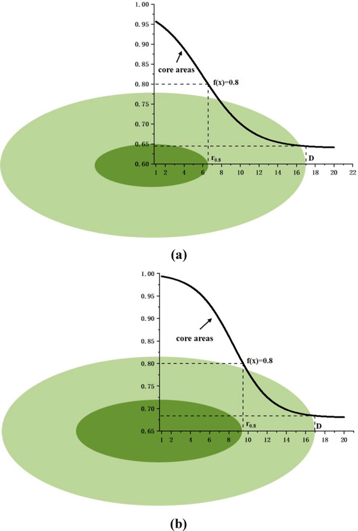
Figure 7. Calculation results of the housing price concentration index. (a) Low percentage of urban core areas (b) High percentage of urban core areas.

Figure 8 presents the calculation results of the housing price concentration index for the 35 cities. The index ranges from 0.267 to 0.576, with Shanghai exhibiting the highest concentration and Changsha the lowest. Combined with the housing price curves in Figure 4, cities with a low concentration index, such as Changsha, Chongqing, Shenyang, and Hefei, exhibit a standard inverse S-shaped curve, where prices decline slowly within the core area. In contrast, cities with a high concentration index, such as Shenzhen, Beijing, Guangzhou, and Shanghai, experience a rapid price decay in the core area. A potential explanation for this pattern is that in cities like Changsha and Chongqing, the overall price level is relatively low and spatially stable, which can be attributed to strong government regulation and a comparatively lower concentration of resources in the urban center. Consequently, the locational premium for proximity to the center is relatively modest. On the other hand, cities like Shenzhen, Beijing, Guangzhou, and Shanghai are characterized by high overall price levels and significant spatial variation. Their urban centers feature a high concentration of diverse resources, granting a substantial premium to nearby neighborhoods. However, this premium effect diminishes sharply with increasing distance from the center, leading to the observed rapid decline in housing prices.

Figure 8

Figure 8. Housing price concentration index for 35 cities.

5 Discussion and conclusion

5.1 Discussion

The function fitting method adopted in this study provides a new approach for quantitative research on the spatial distribution of urban housing prices. The findings contribute to a deeper understanding of the spatial differentiation patterns of intra-urban housing prices. Based on the specific quantitative indicators derived from the inverse S-function parameters, this study offers the following scientific insights and targeted implications for differentiated urban policy formulation.

1. Implementing categorized planning guidance based on the stability and concentration of housing price spatial structures. For cities with high concentration and high stability in housing prices, the steep “core-periphery” gradient reflects excessive functional concentration in the central urban area. The core planning strategy for such cities should focus on cultivating well-functioning sub-centers to promote a transition from a monocentric to a polycentric or networked urban structure, thereby achieving organic decentralization. For example, Shanghai could develop functional sub-centers in suburban areas to redistribute the concentrated population and industries from the core area. For cities with low concentration and low stability in housing prices, the rapid decay of housing prices often indicates insufficient radiating and driving capacity of the central urban area. Therefore, the planning focus should prioritize enhancing the comprehensive service functions and urban vitality of the main urban area, strengthening its role as a growth pole, and improving spatial connectivity between the central and peripheral areas. For instance, Xining could designate and upgrade its municipal-level core commercial districts or public service centers, transforming them into a powerful commercial and business hub.

2. Utilizing quantitative housing price fitting parameters to adjust housing strategies and allocate public services and infrastructure. Housing policies should implement “zonal precision regulation”. For instance, for cities with high concentration, the core high-price areas should prioritize the development of affordable housing to alleviate affordability crises. In contrast, peripheral new areas require preemptive investments in high-quality public services and infrastructure to enhance locational value and guide the rational distribution of population and housing demand. For cities with low concentration and low stability, spatial balanced development can be promoted by deploying high-quality public spaces and improving basic service facilities on the periphery of the central urban area. Additionally, real estate development in peripheral areas should be cautiously controlled to avoid resource waste and spatial value dilution caused by “sprawl-style” expansion. Meanwhile, encouraging the coordinated development of industrial parks and supporting housing can drive steady increases in housing value in peripheral areas through job spillover effects.

This study also has certain limitations. The inverse S-function model primarily captures the macro-level pattern of housing price variation with distance from the city center and does not incorporate micro-level factors such as accessibility to public services or transportation convenience. Future research will also incorporate additional variables to construct a more refined model and strengthen its explanatory power and generalizability through sensitivity analysis and cross-city comparative validation. Moreover, we will explore how urban design and planning interventions influence the inverse S-curve, thereby linking the empirical findings to actionable strategies for improving housing affordability and promoting spatial balance.

5.2 Conclusion

Based on residential community housing price data from 35 major Chinese cities in August 2020, this study quantitatively reveals the spatial decay patterns of intra-urban housing prices using the inverse S-function model and measures their spatial distribution forms through the Stability Index (Sta) and Concentration Index (Ctl). The research of this study is summarized as follows:

1. A qualitative analysis of intra-urban housing prices, based on the global Moran’s I index, reveals that housing prices in residential communities across 35 large cities exhibit a certain degree of spatial autocorrelation, indicating the presence of spatial agglomeration.

2. The inverse S-equation is used to fit the housing prices in 35 cities, and the results show that the average fitting degree of the function is 0.98, indicating that it can fit the spatial variation of housing prices well. The differences in the function parameters indicate the differences in the housing price curves with distance in different cities. The housing price curves can be roughly divided into three forms: three-stage standard inverse S-decay, two-stage fast followed by slow decay, and single-stage linear decay. Typically, cities with a pronounced monocentric structure (e.g., Beijing, Shanghai) exhibit higher housing price concentration (Ctl), meaning the premium effect is highly concentrated within a small core area. In contrast, some polycentric cities (e.g., Changsha, Shenyang) show a more dispersed price distribution. Furthermore, these indices show a notable correlation with urban economic development levels. For instance, economically developed cities (e.g., Nanjing, Tianjin) demonstrate higher spatial stability, with a more gradual decay process, whereas most cities in western and northeastern China (e.g., Xining, Hohhot) show lower stability, with prices dropping rapidly from the center outward.

Data availability statement

The datasets presented in this article are not readily available because this dataset is not publicly available due to confidentiality reasons. Requests to access the datasets should be directed to XL, bGlhbmd4akB3aHUuZWR1LmNu.

Author contributions

XL: Writing – original draft, Writing – review and editing, Methodology, Conceptualization. TQ: Data curation, Writing – review and editing. BJ: Writing – review and editing, Investigation, Funding acquisition. JL: Formal Analysis, Visualization, Writing – review and editing. SG: Writing – review and editing, Software.

Funding

The author(s) declared that financial support was received for this work and/or its publication. The completion of this work was supported by Collaborative Innovation Center for Natural Resources Planning and Marine Technology of Guangzhou (No.2023B04J0301, No.2025B04J0030).

Acknowledgements

Thanks for the support of Academic Specialty Group for Urban Sensing in Chinese Society of Urban Planning.

Conflict of interest

Authors XL, TQ, BJ, and JL were employed by Guangzhou Urban Planning & Design Survey Research Institute Co., Ltd.

Author XL was employed by Guangzhou Liwan Planning, Survey & Design Co., Ltd.

The remaining author(s) declared that this work was conducted in the absence of any commercial or financial relationships that could be construed as a potential conflict of interest

Generative AI statement

The author(s) declared that generative AI was not used in the creation of this manuscript.

Any alternative text (alt text) provided alongside figures in this article has been generated by Frontiers with the support of artificial intelligence and reasonable efforts have been made to ensure accuracy, including review by the authors wherever possible. If you identify any issues, please contact us.

Publisher’s note

All claims expressed in this article are solely those of the authors and do not necessarily represent those of their affiliated organizations, or those of the publisher, the editors and the reviewers. Any product that may be evaluated in this article, or claim that may be made by its manufacturer, is not guaranteed or endorsed by the publisher.

References

Aliyar, A. K., Major, M. D., Tannous, H. O., and Al-Esmail, F. R. (2023). Urban form and real estate value in Msheireb Downtown Doha, Qatar. J. Contemp. Urban Aff. 7 (1), 224–241. doi:10.25034/ijcua.2023.v7n1-15

CrossRef Full Text | Google Scholar

Angel, S., Parent, J., and Civco, D. L. (2010). Ten compactness properties of circles: measuring shape in geography. Can. Geogr./Le Géogr. Canadien 54 (4), 441–461. doi:10.1111/j.1541-0064.2009.00304.x

CrossRef Full Text | Google Scholar

Batty, M., and Kim, K. S. (1992). Form follows function: reformulating urban population density functions. Urban Stud. 29, 1043–1069. doi:10.1080/00420989220081041

CrossRef Full Text | Google Scholar

Borruso, G. (2008). Network density estimation: a GIS approach for analysing point patterns in a network space. Trans. GIS 12 (3), 377–402. doi:10.1111/j.1467-9671.2008.01107.x

CrossRef Full Text | Google Scholar

Chen, F. (2018). Spatial differentiation of urban housing prices in Guangdong province and its influencing factors. Mod. Econ. 9, 664–681. doi:10.4236/me.2018.94043

CrossRef Full Text | Google Scholar

Cheshire, P., and Sheppard, S. (2002). The welfare economics of land use planning. J. Urban Econ. 52 (2), 242–269. doi:10.1016/S0094-1190(02)00003-7

CrossRef Full Text | Google Scholar

Dong, T., Jiao, L., Xu, G., Yang, L., and Liu, J. (2019). Towards sustainability? Analyzing changing urban form patterns in the United States, Europe, and China. Sci. Total Environ. 671, 632–643. doi:10.1016/j.scitotenv.2019.03.269

PubMed Abstract | CrossRef Full Text | Google Scholar

Elgammal, A., Duraiswami, R., Harwood, D., and Davis, L. S. (2002). Background and foreground modeling using nonparametric kernel density estimation for visual surveillance. Proc. IEEE 90 (7), 1151–1163. doi:10.1109/JPROC.2002.801448

CrossRef Full Text | Google Scholar

Fandian, S., and Panwar, M. (2025). Influence of the mass rapid transit system on plotted residential property prices: a case study of Gurugram, India. J. Contemp. Urban Aff. 9 (2), 387–401. doi:10.25034/ijcua.2025.v9n2-4

CrossRef Full Text | Google Scholar

Feng, J., and Zhou, Y. (2003). A review and prospect on urban internal spatial structure research in China. Prog. Geogr. (3), 204–215. doi:10.11820/dlkxjz.2003.03.010

CrossRef Full Text | Google Scholar

Gao, H., Qiao, X., Yang, Y., Liu, L., Zhang, J., Zhou, H., et al. (2025). Modeling urban land density with Gaussian and inverse S functions by analyzing urban expansion in Zhengzhou city. Sci. Rep. 15 (1), 18116. doi:10.1038/s41598-025-03009-4

PubMed Abstract | CrossRef Full Text | Google Scholar

Govind, N. R., and Ramesh, H. (2020). Exploring the relationship between LST and land cover of Bengaluru by concentric ring approach. Environ. Monit. Assess. 192 (10), 650. doi:10.1007/s10661-020-08601-x

PubMed Abstract | CrossRef Full Text | Google Scholar

Gui, B., Bhardwaj, A., and Sam, L. (2024). Revealing the evolution of spatiotemporal patterns of urban expansion using mathematical modelling and emerging hotspot analysis. J. Environ. Manag. 364, 121477. doi:10.1016/j.jenvman.2024.121477

PubMed Abstract | CrossRef Full Text | Google Scholar

Jiao, L. (2015). Urban land density function: a new method to characterize urban expansion. Landsc. Urban Plan. 139, 26–39. doi:10.1016/j.landurbplan.2015.02.017

CrossRef Full Text | Google Scholar

Jiao, L., and Dong, T. (2018). Inverse S-shape rule of urban land density distribution and its applications. Geomatics Inf. Sci. Wuhan Univ. 43 (4), 8–16. (In Chinese). doi:10.14188/j.2095-6045.2018217

CrossRef Full Text | Google Scholar

Kenyon, G. E., Arribas-Bel, D., Robinson, C., Gkountouna, O., Arbués, P., and Rey-Blanco, D. (2024). Intra-urban house prices in Madrid following the financial crisis: an exploration of spatial inequality. Npj Urban Sustain. 4, 26. doi:10.1038/s42949-024-00161-0

CrossRef Full Text | Google Scholar

Laziou, G., Lemoy, R., and Texier, L. M. (2025). Radial analysis and scaling of housing prices in French urban areas. Environ. Plan. B Urban Anal. City Sci. 52 (5), 1147–1162. doi:10.1177/23998083241281890

CrossRef Full Text | Google Scholar

Leslie, T. F. (2010). Identification and differentiation of urban centers in Phoenix through a multi-criteria kernel-density approach. Int. Regional Sci. Rev. 33 (2), 205–235. doi:10.1177/0160017610365538

CrossRef Full Text | Google Scholar

Li, X., Fang, J., and Piao, S. (2003). The comparison of spatial characteristics in urban land use growth among the central and sub-cities in Shanghai region. Geogr. Res. 22 (6), 769–779.

Google Scholar

Li, Z., Jiao, L., Zhang, B., Xu, G., and Liu, J. (2021). Understanding the pattern and mechanism of spatial concentration of urban land use, population and economic activities: a case study in Wuhan, China. Geo-spatial Inf. Sci. 24 (4), 678–694. doi:10.1080/10095020.2021.1978276

CrossRef Full Text | Google Scholar

Manzoli, E., and Mocetti, S. (2019). The house price gradient: evidence from Italian cities. Italian Econ. J. 5 (2), 281–305. doi:10.1007/s40797-019-00094-z

CrossRef Full Text | Google Scholar

Niu, F. (2008). Introduction to urbanology. Beijing, China: China Social Sciences Press. (In Chinese).

Google Scholar

Reinhart, C. M., and Rogoff, K. S. (2009). This time is different: eight centuries of financial folly. Princeton University Press.

Google Scholar

Song, C., Chen, J., Li, C., and Ai, G. (2020). Urban vitality zone and central district identification based on big data: a case study in Guangzhou city. Urban Transp. China 18 (4), 71–78. (In Chinese). doi:10.13813/j.cn11-5141/u.2020.0028

CrossRef Full Text | Google Scholar

Sun, Y., Fan, H., Li, M., and Zipf, A. (2016). Identifying the city center using human travel flows generated from location-based social networking data. Environ. Plan. B Plan. Des. 43 (3), 480–498. doi:10.1177/0265813515617642

CrossRef Full Text | Google Scholar

Veneri, P. (2013). The identification of sub-centres in two Italian metropolitan areas: a functional approach. Cities 31, 177–185. doi:10.1016/j.cities.2012.04.006

CrossRef Full Text | Google Scholar

Wang, Y., and Yang, J. (2024). The spatio-temporal development and influencing factors of urban residential land prices in Hebei Province, China. Land 13 (8), 1234. doi:10.3390/land13081234

CrossRef Full Text | Google Scholar

Wang, F., Gao, X. L., and Yan, B. Q. (2014). Research on urban spatial structure in Beijing based on housing price. Prog. Geogr. 33 (10), 1322–1331.

Google Scholar

Wang, Z., Zhao, Y., and Zhang, F. (2022). Simulating the spatial heterogeneity of housing prices in Wuhan, China, by regionally geographically weighted regression. ISPRS Int. J. Geo-Information 11 (2), 129. doi:10.3390/ijgi11020129

CrossRef Full Text | Google Scholar

Xu, G., Dong, T., Cobbinah, P. B., Jiao, L., Sumari, N. S., Chai, B., et al. (2019a). Urban expansion and form changes across African cities with a global outlook: spatiotemporal analysis of urban land densities. J. Clean. Prod. 224, 802–810. doi:10.1016/j.jclepro.2019.03.276

CrossRef Full Text | Google Scholar

Xu, G., Jiao, L., Yuan, M., Dong, T., Zhang, B., and Du, C. (2019b). How does urban population density decline over time? An exponential model for Chinese cities with international comparisons. Landsc. Urban Plan. 183, 59–67. doi:10.1016/j.landurbplan.2018.11.005

CrossRef Full Text | Google Scholar

Yang, J., Li, J., Xu, F., Li, S., Zheng, M., and Gong, J. (2022). Urban development wave: understanding physical spatial processes of urban expansion from density gradient of new urban land. Comput. Environ. Urban Syst. 97, 101867. doi:10.1016/j.compenvurbsys.2022.101867

CrossRef Full Text | Google Scholar

Yoğurtçu, F., and Köksal, A. (2024). District-based rental value coefficients for shopping mall development in Istanbul. J. Contemp. Urban Aff. 8 (2). doi:10.25034/ijcua.2024.v8n2-11

CrossRef Full Text | Google Scholar

Yu, W., Ai, T., and Shao, S. (2015). The analysis and delimitation of central business district using network kernel density estimation. J. Transp. Geogr. 45, 32–47. doi:10.1016/j.jtrangeo.2015.04.008

CrossRef Full Text | Google Scholar

Yu, W., Ai, T., Yang, M., and Liu, J. (2016). Detecting “hot spots” of facility POIs based on kernel density estimation and spatial autocorrelation technique. Geomatics Inf. Sci. Wuhan Univ. 41 (2), 221–227. (In Chinese). doi:10.13203/j.whugis20140092

CrossRef Full Text | Google Scholar

Zhang, H., and Wang, S. (2025). Research on the impact of rail transit accessibility on housing prices: a case study of Chengdu city. J. Green Sci. Technol. 27 (9), 182–186. (In Chinese). doi:10.16663/j.cnki.lskj.2025.09.040

CrossRef Full Text | Google Scholar

Zheng, M., Huang, W., Xu, G., and Jiao, L. (2023). Spatial gradients of urban land density and nighttime light intensity in 30 global megacities. Humanit. Soc. Sci. Commun. 10 (1), 1–11. doi:10.1057/s41599-023-01884-8

CrossRef Full Text | Google Scholar