

- 1 Intelligent Data Analysis Group, Fraunhofer FIRST, Berlin, Germany
- 2 Machine Learning Group, Technical University Berlin, Berlin, Germany
Estimating brain connectivity and especially causality between different brain regions from EEG or MEG is limited by the fact that the data are a largely unknown superposition of the actual brain activities. Any method, which is not robust to mixing artifacts, is prone to yield false positive results. We here review a number of methods that allow for addressing this problem. They are all based on the insight that the imaginary part of the cross-spectra cannot be explained as a mixing artifact. First, a joined decomposition of these imaginary parts into pairwise activities separates subsystems containing different rhythmic activities. Second, assuming that the respective source estimates are least overlapping, yields a separation of the rhythmic interacting subsystem into the source topographies themselves. Finally, a causal relation between these sources can be estimated using the newly proposed measure Phase Slope Index (PSI). This work, for the first time, presents the above methods in combination; all illustrated using a single, simulated data set.
1. Introduction
Electroencephalography (EEG) can directly measure ongoing brain activity with very high temporal but low spatial resolution. In the past decades the main focus was the analysis of event related potentials, i.e., the average brain response to a given stimulus. More recently, the variability of brain activity and especially its interpretation as signatures from the brain as a dynamical network has attracted many researchers (Daglish et al., 2005; Womelsdorf and Fries, 2006; Buckner and Vincent, 2007; Damoiseaux and Greicius, 2009; Fries, 2009; Miller et al., 2009).
Studying brain connectivity using noninvasive electrophysiological measurements like EEG or MEG faces the challenge that the data are largely unknown mixtures of activities of brain sources.
To address this issue, we suggest to construct estimates of brain connectivity from quantities that are unbiased by non-interacting sources. For zero mean data1 the linear statistical signal properties can be determined by the cross-spectral matrices S(f) defined as

where xm(f) are the Fourier transforms at frequency f in channel m for a given segment or trial and 〈·〉 denotes the expectation value which is typically approximated by an average over the segments or trials.
It is straight forward to show that noninteracting sources do not contribute systematically, i.e., apart from random fluctuations around zero to the imaginary part of the cross-spectra,  (S(f)), regardless of the number of sources and details of the forward mapping (Nolte et al., 2004). The reason is that the forward mapping is essentially instantaneous and does not induce phase delays to excellent approximation (Stinstra and Peters, 1998) which would be necessary to yield a nonvanishing imaginary part of S(f).
From the cross-spectra S(f) one can construct coherency matrices C(f), which are a normalized version of S(f), as

In contrast to the imaginary parts of the cross-spectra, (C(f)) also depends on independent sources through the denominator in Eq. 2. However, independent sources can only lead to a decrease of (C(f)) and hence also (C(f)) reflects true interaction even though the physiological interpretation is not trivial especially when interpreting differences of (C(f)), e.g., between different tasks.
Based on these observations we suggested a series of methods to identify and localize brain interactions (Meinecke et al., 2005; Nolte et al., 2006; Stam et al., 2007; Marzetti et al., 2008; Nolte et al., 2009). Additionally, we proposed a method to identify causal structures of the dynamical system under study (Nolte et al., 2008). We here give a brief review of some of these methods (Nolte et al., 2006; Marzetti et al., 2008; Nolte et al., 2008) to identify interacting brain sources and to estimate causal relationships. All the methods will be demonstrated using simulated data whose characteristics are defined in the following section.
2. Simulated Interacting Neural Data
We simulated a seminal case with four dipolar sources as shown in Figure 1, in which the dipoles have all a parallel orientation and are spatially well separated. The sources on the right (left) are interacting with each other but not with the sources on the left (right). We thus considered two interacting subsystems. For both subsystems the source in the back served as driver while the activity of the more frontal sources appeared merely identical to the ones of the drivers but the activity was delayed by 20 ms. The activity of the right driver was given as
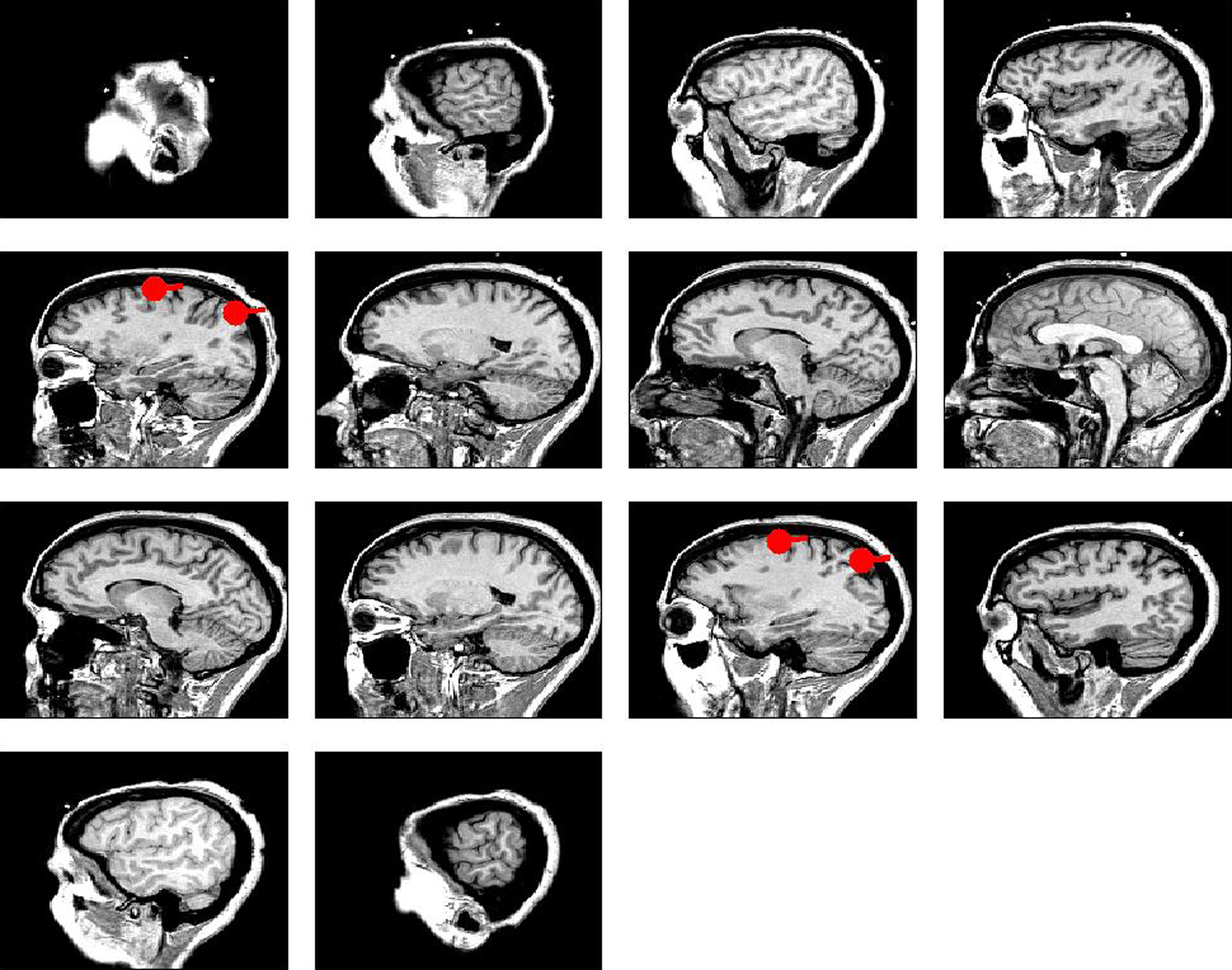
Figure 1. Four dipolar sources overlayed on MRI-slices.

where ξ1(t) is white Gaussian noise with standard deviation 1. Similarly, the activity of the driver on the left side was simulated via

We defined a single time step to equal 10 ms, i.e., we considered a sampling rate of 100 Hz, by which the time series u1(t) and u2(t) displayed pronounced spectral peaks at around 8 and 12 Hz, respectively, and had roughly identical magnitudes. Both time series also have (weak) higher harmonics at 24 and 36 Hz, respectively.
The frontal sources, v1(t) and v2(t) for right and left side, respectively, are merely delayed versions of the drivers:

corresponding to a delay of 20 ms. In total, we modeled 200 s of EEG data.
The activities of the four dipolar sources were mapped into 118 EEG channels equally distributed on the scalp. As volume conductor we assumed a three-shell realistic model calculated from the MRI data containing brain, skull, and scalp with equal conductivities for brain and scalp and 50:1 conductivity ratio between scalp and skull. The Maxwell equations were solved using a semianalytic expansion of the electric lead fields (Nolte and Dassios, 2005). An accurate forward model is important but difficult. For the sake of simplicity we here assumed that the forward model is correct, i.e., for the inverse methods we used the same forward model as for the forward simulation.
To the activities of the sources of interest we superimpose spatially correlated and temporally white noise generated as the activity of a collection of dipoles placed on a 1 cm grid within the entire brain. All components of all dipoles were modeled as iid Gaussian noise leading to highly correlated noise in the EEG electrodes. The noise level was chosen such that the average of power over all channels and frequencies was 20 times higher than the respective average of the signal of interest. In “good” channels and at peak frequencies the power of the signal of interest was still around 10 times higher than the noise.
Power (imaginary part of coherency) over all channels (pairs of channels) are shown as function of frequency in Figure 2. The spatial distribution of the imaginary part of coherency at 10 Hz, i.e., between the peaks and with contributions from both interacting subsystems, is shown in Figure 3.
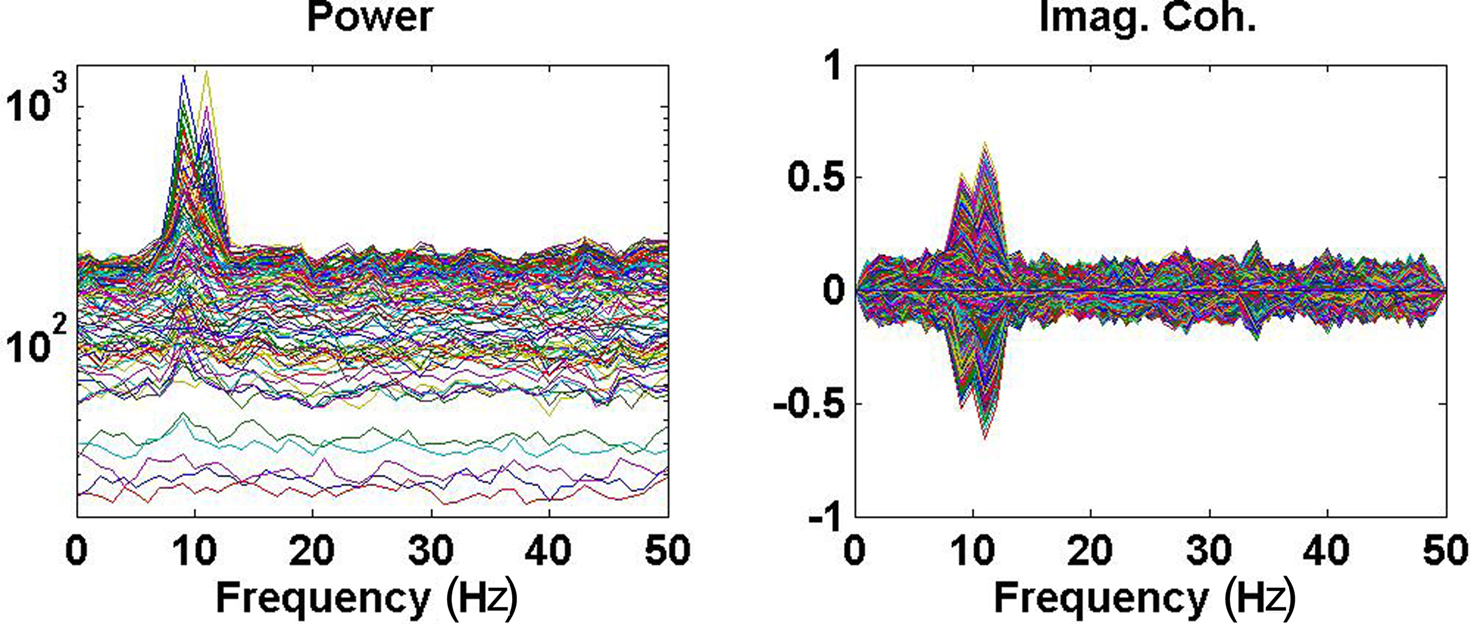
Figure 2. Left: Power over all channels. Right: Imaginary part of coherency over all pairs of channels.

Figure 3. Imaginary part of coherency at 10 Hz. Each small circle corresponds to one row of the coherency matrix.
3. Methods
3.1. Pairwise Interacting Component Analysis (PISA)
In general, EEG data are a superposition of many subsystems including (effectively) independent sources but also interacting rhythmic sources of various physiological content. To separate these systems we assumed that (a) all interactions are pairwise and that (b) there are not more interacting sources than channels. These two assumptions are a clear simplification of the true brain dynamics, but they yield a unique decomposition of the data and may capture the most relevant aspects of the interaction observed in EEG data, at least when focussing on the current discussion. These assumptions can be expressed for an even number of N channels as a model for the imaginary part of the cross-spectra:

For each k the set of topographies (ak and bk) and the “interaction spectrum” Pk(f) form a – what we call – PISA component. We note that this model is only unique up to linear mixing of the two topographies for each k. In other words, the model only identifies the 2D-subspace spanned by the two topographies and not the individual components.
The model is found by joined diagonalization (cf. Ziehe et al., 2004) of (S(f)) in the complex domain: we find a demixing matrix W such that W(S(f))W† is diagonal. It can be shown that real and imaginary parts of the columns of the mixing matrix A = W−1 span the same subspaces as the pairs of topographies ak and bk. For technical details we refer to Nolte et al. (2006).
Results of the PISA decomposition for the simulated data set are shown in Figure 4, where we show the largest three components. Only the first and the second component revealed a significant interaction spectrum corresponding to the two interacting subsystems in the left and right hemisphere, respectively.
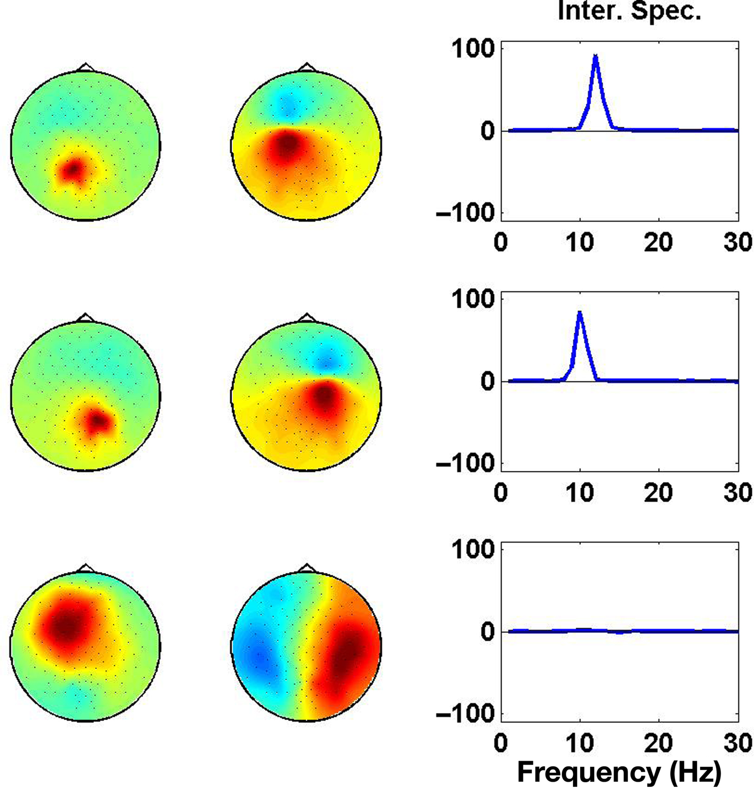
Figure 4. Each row displays the result for one PISA Component. Left and middle columns show the respective topographies. Panels in the right column show the interaction as a function of frequency.
3.2. Minimum Overlap Component Analysis (MOCA)
In order to uniquely decompose the 2D-subspaces found by the PISA method into contributions from individual sources we must introduce further spatial constraints on the nature of the sources. To this end we apply a linear inverse operator, e.g., a minimum norm solver G onto the topographies denoted here for any fixed k as x1 = ak and x2 = bk, such that the topographies are mapped into distributions si of the source field

where si = si(m,k) is a three dimensional vector field calculated in brain voxels m = 1,..,M and in directions k = 1,..,3. The distributions do not represent the sources of the brain, denoted as qi, but are, within the accuracy of the inverse method, a yet unknown superposition of them:

for i = 1,2. The 2 × 2 mixing matrix H can be calculated uniquely under the following constraints
1. The sources are orthonormal:

2. The sources have minimum overlap:

This cost function first squares the scalar product of two dipole moments at each voxel and then sums these squares over all voxels. It vanishes if the two dipole distributions have disjoint support (i.e., disjoint regions of non-vanishing activity), thus measuring overlap. It also vanishes if the orientations at each voxel are orthogonal and therefore corresponds to a weaker form of overlap allowing in principle also activities at the same location as long as the orientations are sufficiently different. Thus, a strong bias toward remote interaction is removed.
The minimization in Eq. 10 can be realized analytically (Marzetti et al., 2008). If the concept is generalized to more than two topographies the minimization requires a numerical approach, which, however, is surprisingly fast and robust (Nolte et al., 2009). We note that the spatial constraints (Eqs 9 and 10) and the methods to solve the minimization are similar to those used in ICA in the context of fMRI data analysis (McKeown and Sejnowski, 1998; Matsuda and Yamaguchi, 2004) with the major difference that we here decompose vector fields rather than scalar ones. In particular, the orthogonality constraint in Eq. 9 corresponds, mutatis mutandis, to “sphering” as is used in most ICA methods also used for EEG/MEG data analysis: for simplicity, the data are transformed to be exactly uncorrelated while independence in higher statistical orders is only forced to be as good as possible.
For the present data set we further assumed the sources to be located on the cortex but allowed for arbitrary orientation. Source estimates of the first two PISA components for the simulated data set are shown in Figure 5. We observe that each of the topographies, decomposed from the PISA results using MOCA, corresponds to one of the simulated dipoles.
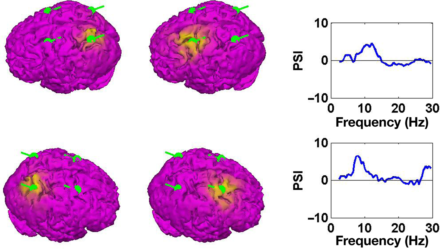
Figure 5. Left and middle panels: estimated sources of the PISA components. Right panels: causal structure as function of function. Positive results indicate that the sources shown in the left panels drive those shown in the middle panels.
3.3. Phase Slope Index (PSI)
We finally want to estimate causal structures between the estimated sources. Since the combination of PISA and MOCA resulted in a complete basis of topographies we can find the source activities by applying the inverse of the respective matrix onto the data.
The “Phase Slope Index” (PSI) estimates the causal structure between any two source activities. It is defined as Nolte et al. (2008)

where Cij(f) is the complex coherency between sources i and j, as given in Eq. 2, and δf is the frequency resolution of the coherency. F is the set of frequencies over which the slope is summed. Usually, F contains all frequencies, but it can also be restricted to a specified band for rhythmic activities.
To see that the definition of  corresponds to a meaningful estimate of the average slope it is convenient to rewrite it as

with Cij(f) = αij(f)exp(iΦ(f)) and αij(f) = |Cij(f)| being frequency dependent weights.
For smooth phase spectra, sin(Φ(f + δf) − Φ(f)) ≈ Φ(f + δf) − Φ(f) and hence  corresponds to a weighted average of the slope.
We list the most important qualitative properties of  :
:
1. For an infinite amount of data and for arbitrary instantaneous mixtures of an arbitrary number of independent sources,  is exactly zero, because mixtures of independent sources do not induce an imaginary part of coherencies (Nolte et al., 2004) which in turn is necessary to generate a non-vanishing
  . For finite data,
  will then fluctuate in this case around zero within error bounds. A special case of this are phase jumps from 0 to ±π which can arise also for mixtures of independent sources.
2.  is expressed in terms of coherencies, only. The standard deviation of a coherency is approximately constant and only depends on the number of averages which is equal for all frequencies. Thus, large but meaningless phase fluctuations in frequency bands containing essentially independent signals are largely suppressed.
3. If the phase Φ(f) is linear in f and provided that the frequency resolution is sufficient (i.e., δf is sufficiently small), the argument in the sum has the same sign across all frequencies and then  will have the same sign as the slope of Φ(f).
It is convenient to normalize  by an estimate of its standard deviation

with  being estimated by the Jackknife method, which we validated in own simulations. In the examples below we consider absolute values of each larger than 2 as significant.
It is important to point out that the phase of coherency itself is not interpreted in terms of causality. For example, a phase of π/2 switches to −π/2 if the sign of one of the signals is reversed, but the PSI measure is invariant with respect to the sign of the signals. Rather than on phase, PSI is based on the slope of the phase as a function of frequency. Note, that a sign change adds a constant to the phase and has no effect on the slope. The method assumes that the studied frequency range properly covers the dynamical range. For purely periodic signals, any causality estimate would be dubious. In that case Ψ would be insignificant because negative and positive slopes cancel.
Results for the causal structure of the sources estimated from the simulated data are shown in the right panels of Figure 5. To calculate PSI we chose segments of length 2 s corresponding to a frequency resolution of δf = 0.5 Hz. We observe that in both cases the source in the back is estimated as the driver.
4. Conclusion
Accurately measuring the interaction of oscillatory brain sources from EEG/MEG is a challenge. Due to the well-known effects of volume conduction, it is easy and not uncommon to detect spurious interaction and thus reach spurious neuroscientific insight. The present review has assembled three data analytical techniques that avoid such erroneous conclusions as they are based on the imaginary parts of the cross-spectra S(f) that – as outlined above – immunizes analysis against volume conduction artifacts. To clarify this basic message we have used simulated EEG data from interacting neural systems and took the reader through three essential analysis steps (a) discovering interacting sources by PISA, (b) localizing them under constraints by MOCA and (c) estimating their causal relationship by PSI.
Future research will extend the studies on causal relations of interacting sources also for high noise situations (cf. Nolte et al., 2010) and nonstationary processes (cf. von Bünau et al., 2009) and the broad application of the presented computational methods in the neurosciences.
Conflict of Interest Statement
The authors declare that the research was conducted in the absence of any commercial or financial relationships that could be construed as a potential conflict of interest.
Acknowledgments
The authors gratefully acknowledge financial support by EU, BMBF, and DFG. We would like to thank our co-authors for their permission to use material from joint publications.
Footnote
- ^In an event related design the mean can be subtracted.
References
Buckner, R. L., and Vincent, J. L. (2007). Unrest at rest: default activity and spontaneous network correlations. Neuroimage 37, 1091–1096.
Daglish, M., Lingford-Hughes, A., and Nutt, D. (2005). Human functional neuroimaging connectivity research in dependence. Rev. Neurosci. 16, 151–157.
Damoiseaux, J. S., and Greicius, M. D. (2009). Greater than the sum of its parts: a review of studies combining structural connectivity and resting-state functional connectivity. Brain Struct. Funct. 213, 525–533.
Fries, P. (2009). Neuronal gamma-band synchronization as a fundamental process in cortical computation. Annu. Rev. Neurosci. 32, 209–224.
Marzetti, L., Del Gratta, C., and Nolte, G. (2008). Understanding brain connectivity from EEG data by identifying systems composed of interacting sources. Neuroimage 42, 87–98.
Matsuda, Y., and Yamaguchi, K. (2004). “Semi-invariant function of Jacobi algorithm in independent component analysis,” in Proceedings of IEEE International Joint Conference on Neural Networks, Budapest.
McKeown, M. J., and Sejnowski, T. J. (1998). Independent component analysis of fMRI data: examining the assumptions. Hum. Brain Mapp. 6, 368–372.
Meinecke, F., Ziehe, A., Kurths, J., and Müller, K. R. (2005). Measuring phase synchronization of superimposed signals. Phys. Rev. Lett. 94, 084102.
Miller, K. J., Weaver, K. E., and Ojemann, J. G. (2009). Direct electrophysiological measurement of human default network areas. Proc. Natl. Acad. Sci. U.S.A. 106, 12174–12177.
Nolte, G., Bai, U., Weathon, L., Mari, Z., Vorbach, S., and Hallet, M. (2004). Identifying true brain interaction from EEG data using the imaginary part of coherency. Clin. Neurophysiol. 115, 2294–2307.
Nolte, G., and Dassios, G. (2005). Analytic expansion of the EEG lead field for realistic volume conductors. Phys. Med. Biol. 50, 3807–3823.
Nolte, G., Marzetti, L., and Valdes Sosa, P. (2009). Minimum overlap component analysis (MOCA) of EEG/MEG data for more than two sources. J. Neurosci. Methods 183, 72–76.
Nolte, G., Meinecke, F. C., Ziehe, A., and Müller, K. R. (2006). Identifying interactions in mixed and noisy complex systems. Phys. Rev. E 73, 051913.
Nolte, G., Ziehe, A., Krämer, N., Popescu, F., and Müller, K. R. (2010). Comparison of granger causality and phase slope index, JMLR Workshop Con. Proc. 6, 267–276.
Nolte, G., Ziehe, A., Nikulin, V. V., Schlögl, A., Krämer, N., Brismar, T., and Müller, K. R. (2008). Robustly estimating the flow direction of information in complex physical systems. Phys. Rev. Lett. 100, 234101.
Stam, C. J., Nolte, G., Daffertshofer, A. (2007). Phase lag index: assessment of functional connectivity from multi channel EEG and MEG with diminished bias from common sources. Hum. Brain Mapp. 28, 1178–1193.
Stinstra, J. G., and Peters, M. J. (1998). The volume conductor may act as a temporal filter on the ECG and EEG. Med. Biol. Eng. Comput. 36, 711–716.
von Bünau, P., Meinecke, F. C., Kiraly, F., and Müller, K. R. (2009). Finding stationary subspaces in multivariate time series. Phys. Rev. Lett. 103, 214101.
Keywords: EEG, volume conduction, causality, interaction, PISA, MOCA, PSI
Citation: Nolte G and Mueller KR (2010) Localizing and estimating causal relations of interacting brain rhythms. Front. Hum. Neurosci. 4:209. doi: 10.3389/fnhum.2010.00209
Received: 31 May 2010;
Accepted: 09 October 2010;
published online: 22 November 2010.
Edited by:
Kai J. Miller, University of Washington, USAReviewed by:
Pedro Valdes-Sosa, Cuban Neuroscience Center, USAAndreas Daffertshofer, VU University Amsterdam, Netherlands
Copyright: © 2010 Nolte and Mueller. This is an open-access article subject to an exclusive license agreement between the authors and the Frontiers Research Foundation, which permits unrestricted use, distribution, and reproduction in any medium, provided the original authors and source are credited.
*Correspondence: Guido Nolte, Intelligent Data Analysis Group, Fraunhofer FIRST, Kekul estr. 7, 12489 Berlin, Germany. e-mail:bm9sdGVAZmlyc3QuZmhnLmRl