Modular organization of brain resting state networks in chronic back pain patients

Recent work on functional magnetic resonance imaging large-scale brain networks under resting conditions demonstrated its potential to evaluate the integrity of brain function under normal and pathological conditions. A similar approach is used in this work to study a group of chronic back pain patients and healthy controls to determine the impact of long enduring pain over brain dynamics. Correlation networks were constructed from the mutual partial correlations of brain activity’s time series selected from ninety regions using a well validated brain parcellation atlas. The study of the resulting networks revealed an organization of up to six communities with similar modularity in both groups, but with important differences in the membership of key communities of frontal and temporal regions. The bulk of these findings were confirmed by a surprisingly naive analysis based on the pairwise correlations of the strongest and weakest correlated healthy regions. Beside confirming the brain effects of long enduring pain, these results provide a framework to study the effect of other chronic conditions over cortical function.

I. Introduction

Since the initial work of Eguiluz et al. (2005), complex networks has been widely used to represent functional brain networks. Within this approach, resting state experiments have been analyzed at different scales, either defining nodes as voxels (van den Heuven et al., 2008) or anatomical regions based on a prior automated anatomical labeling (AAL) atlas (Salvador et al., 2005). The organization of resting state brain activity in groups of networks or modules has been studied using different strategies, ranging from univariate analysis as seed correlation (Fox et al., 2005, for example), multivariate linear approaches, as probabilistic independent component analysis (ICA) (Beckmann et al., 2005; Smith et al., 2009) and modular organization in complex networks (Stanberry et al., 2008; Meunier et al., 2009a,b). These analyses has been useful to evaluate the integrity of brain function under normal (Damoiseaux et al., 2006) and pathological conditions (Broyd et al., 2009), including Alzheimer disease (He et al., 2008), schizophrenia (Garrity et al., 2007), and epilepsy (Laufs et al., 2007; Lui et al., 2008), but has not been used in analyzing chronic back pain (CBP) condition.

The experience of pain is usually associated with the activation of a large distributed brain network called the “pain matrix,” which includes somatosensory, insular, anterior cingulate and prefrontal cortices, as well as the thalamus (Tracey and Mantyh, 2007). Moreover, previous neuroimaging studies indicate that enduring chronic pain seems to induce a pronounced activation of the pain matrix (Witting et al., 2006) and to alter brain dynamics beyond the feeling of pain itself (Baliki et al., 2008). A recent work (Tagliazucchi et al., 2010) has further reported for the first time alterations in resting state networks of patients with CBP, motivating further work to evaluate possible global changes in their brain modular organization. This is a significant aim, given that patients with chronic pain suffer from a myriad of symptoms including sleep disturbances, depression, cognitive and attention deficits, etc (Apkarian et al., 2004), whose neurophysiological mechanisms are not yet well understood. Thus, in this paper we use fMRI to identify alterations of brain resting state networks in patients with CBP compared with healthy controls (HC). The modular organization of these networks in both groups is analyzed and significant changes in the communities are contrasted within a pairwise correlations approach.

The paper is organized as follows: Section II describes the experimental conditions. Section II A includes the numerical methods used to construct the functional networks of brain activity and section II B the definition of modularity, node regional roles, and a brief description of the community detection algorithm. Section III describes the community structure of brain functional networks found in both groups together with a detailed analysis of their main features (section III A). Then, a heuristic analysis (section III B) is used to explain the global alterations found in community organization in terms of changes in pairwise correlations. Finally, the identification of the key regions playing a major role in the community organization (section III C) is analyzed. The paper concludes with a discussion of the main alterations found and its consistency with previous findings.

II. Materials and Methods

Twelve patients with CBP (29–67 years old, mean ± SD = 51.2 ± 11.2) and 12 HC subjects (21−60 years old, mean ± SD = 40.2 ± 12.7) participate in the study. Age differences between both groups are not significant (p < 0.05). The study was approved by the Northwestern University IRB committee. All participants were right-handed and completed the Depression and the Anxiety Beck’s questionnaires, as well as several pain-related data which have been already published elsewhere (Baliki et al., 2006). As already reported in a previous study the depression and anxiety scores in both groups were far away from pathological criteria, and no group differences were observed on these scores. Participants were scanned following a typical brain resting state protocol (Fox and Raichle, 2007), in which the subject is lying in the scanner and asked to keep their mind blank, eyes closed and avoid falling asleep. Functional magnetic resonance data was acquired in all cases using a 3T Siemens Trio whole-body scanner with echo-planar imaging capability using the standard radio-frequency head coil (scanning parameters were similar to those used in an earlier study, Baliki et al., 2008).

In each subject, a total of 300 images were obtained spaced by 2.5 s. in which the brain oxygen level dependent (BOLD) signal is recorded for each one of the 64 × 64 × 49 sites (so-called voxels of dimension 3.4375 mm × 3.4375 mm × 3 mm). Preprocessing of BOLD signal was performed using FMRIB Expert Analysis Tool (FEAT, Jezzard et al., 2001), http://www.fmrib.ox.ac.uk/fsl), involving motion correction using MCFLIRT; slice-timing correction using Fourier-space time series phase-shifting; non-brain removal using BET; spatial smoothing using a Gaussian kernel of full-width-half-maximum 5 mm. Brain images were normalized to standard space with the MNI 152 (average brain image constructed from 152 normal subjects at Montreal Neurological Institute) template using FMRIB’s linear image registration tool (FLIRT)¹. Data was band pass filtered (0.01–0.1 Hz) using a 0 lag band pass frequency filter in order to avoid low frequency noise (e.g., scanner drift) and high frequency artifacts (Cordes et al., 2000, 2001). An ICA denoising procedure (Beckmann and Smith, 2004) consisting in removal edges and high frequency artifacts by linear regression was done using Melodic (PICA). The data was parceled using anatomical regions based on a prior AAL atlas (Tzourio-Mazoyer et al., 2002). This parcellation divides each cerebral hemisphere into 45 anatomical regions. Regional mean time series were estimated for each individual by averaging the BOLD time series over all voxels in each of the 90 regions, which are used to construct the correlation networks.

A. Networks Construction

Inherent to the idea behind computing community’s properties is the assumption that brain activity can be described as the flow of activity on a dynamic network (Sporns et al., 2004; Salvador et al., 2005; Eguiluz et al., 2005; Achard and Bullmore, 2007; Bullmore and Sporns, 2009; Meunier et al., 2009b). The first step in this direction is to extract the network from the fMRI data. This is shown schematically in Figure 1, where interactions between the ninety regions (Tzourio-Mazoyer et al., 2002) are defined by their mutual co-activity, estimated using partial correlations (Figure 1A). Following (Soranzo et al., 2007), the minimum first order partial correlation between X and Y is calculated as,

FIGURE 1

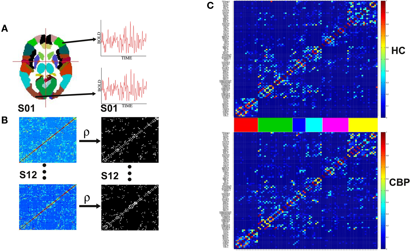
Figure 1. Steps involved in the construction of brain correlation networks. (A) Average BOLD activity time series for each of the 90 anatomical regions defined in (Tzourio-Mazoyer et al., 2002) are extracted. (B) Partial correlation matrices (Eq. 1) for each of the twelve subjects in each group (left) and adjacency matrices (right) with 1 if two regions have a correlation larger than a certain threshold and 0 otherwise. (C) The weighted group networks obtained from the correlation matrices of the healthy control (HC) (top) and chronic back pain (CBP) (bottom) subjects. The color bars between the panels identify the six communities of the HC group. Same ordering is used for the CBP group.

where

and R(X,Y) is the linear correlation given by

where 〈..〉 is a temporal average and σ(X(t)) is the standard deviation of X(t). These calculations result in a 90 × 90 matrix for each subject (Figure 1B). To define a graph, each matrix is thresholded to create an adjacency matrix A where the element is either 1 if the value of the partial correlation is greater than a given threshold ρ or 0 otherwise (Figure 1B).

The threshold level is a critical parameter in this kind of analysis. Very small ρ values will produce highly connected networks in which the presence of well defined communities (i.e., group of nodes which are more densely connected amongst them than with the rest of the network) will be hindered. On the other hand, for very high levels of ρ a disconnected network could appear. Since there is not a priori scale to choose the ρ’s level, we consider a range of threshold values to get networks with a given fixed number of edges, ranging from N_L = 100 up to N_L = 400 links (ρ ∼ 0.6−0.9) as was previously done in (Meunier et al., 2009a).

To compare networks between different groups (i.e., healthy subjects or patients) the data can be collapsed into an average correlation matrix for each group (see Meunier et al., 2009a, for example). This results on a single graph for each group, but the information about variability within each group is lost. To overcome this issue, we compute weighted networks calculated as the average of binary networks of all subjects in the group. The corresponding connectivity matrix reads as:

where n_p is the number of patients in a given group and Θ(X) is the Heaviside step function (Θ(X) is 1 if X ≥ 0 and 0 if X < 0). This means that if partial correlations R_C between regions i and j in a given subject p is above threshold, it contributes with 1/n_p to the weight of group matrix between regions i and j.

Figure 1C shows the weighted networks estimated from N_L = 200 binary networks for both groups. Regions are sorted according to the community structure found in HC group (see Section 2.2) and their location in the adjacency matrix colored to facilitate their identification in subsequent figures. The differences in network community’s organization are described in section III.

B. Modularity

The definition of a network module is usually given in terms of the subset of graph’s nodes which are more densely connected among them than with the rest of the network (Newman and Girvan, 2004). Several algorithms have been proposed to detect these modules in weighted complex networks (Clauset et al., 2004; Newman, 2004; Duch and Arenas, 2005). A common approach is to maximize a quantity that estimates the differences between the actual number of intramodule links and the expected number for the same modules in a randomized network. This quantity, called modularity (Q), can be expressed as:

where A_i,j is the adjacency weighted matrix, is the number of links of the network and is the degree of node i (Newman, 2004; Ahnert et al., 2007) and c_i is the community i.

To find communities in brain functional networks we use the algorithm developed by Duch and Arenas (2005), which perform an heuristic search procedure based on extremal optimization (Boettcher and Percus, 2001a,b) to find the network community configuration with the best modularity value.

C. Region’s Roles

In a community-structured network, certain nodes might play more important roles than others in the organization of these structures. A fruitful approach to quantify this contribution is to track the intra-modular degree and the participation coefficient of each node (Guimera and Amaral, 2005). The intra-modular degree is a measure of how well connected is a node compared with other nodes of the same community and its z-score can be computed as,

with κ_i the intra-modular degree of the ith node, i.e., the number of links of node i to other nodes in its module c_i, as the average of κ_i over all nodes in module c_i and the standard deviation of κ in c_i.

The participation coefficient quantifies the balance between the intra-module versus inter-module connectivity for a given node. It is defined as

where κ_ic is the number of links of node i to nodes in module c and k_i is the degree of node i. If all the links of node i fall within its own module, then κ_ic = k_i and the participation coefficient is 0. On the other hand, if all the links of node i are distributed among all other modules, P_i approaches one.

Considering these two definitions, nodes with high intra-modular degree are considered hubs, while nodes with high participation coefficients are called connectors. These definitions are used here to identify the regions which play key roles in the organization of brain activity at resting state.

III. Results

In this section we will show the results related with the analysis of the structure of functional brain networks. First, we will describe the communities found in both groups, their stability properties and their functional implications. Second, we will analyze which changes in pairwise correlation explains the alterations seen in the CBP communities, and finally we will identify the regions which play key roles in module’s organization.

A. Communities

The algorithm used to search for partitions which maximizes the network modularity is shown schematically in Figure 2A. For the two groups studied as well as for an equivalent random networks, the maximum modularity values are shown in Figure 2B as a function of N_L = (N_L 100–400). Notice that both networks show values of Q_max larger than their equivalent random networks, implying a highly modular structure. Although Q_max depends on N_L, no significant differences where found between HCP and CBP, for any given N_L. The number of detected modules as a function of N_L is shown in Figure 2C. The number of communities stabilizes for N_L ≥ 200 and is similar for both groups.

FIGURE 2

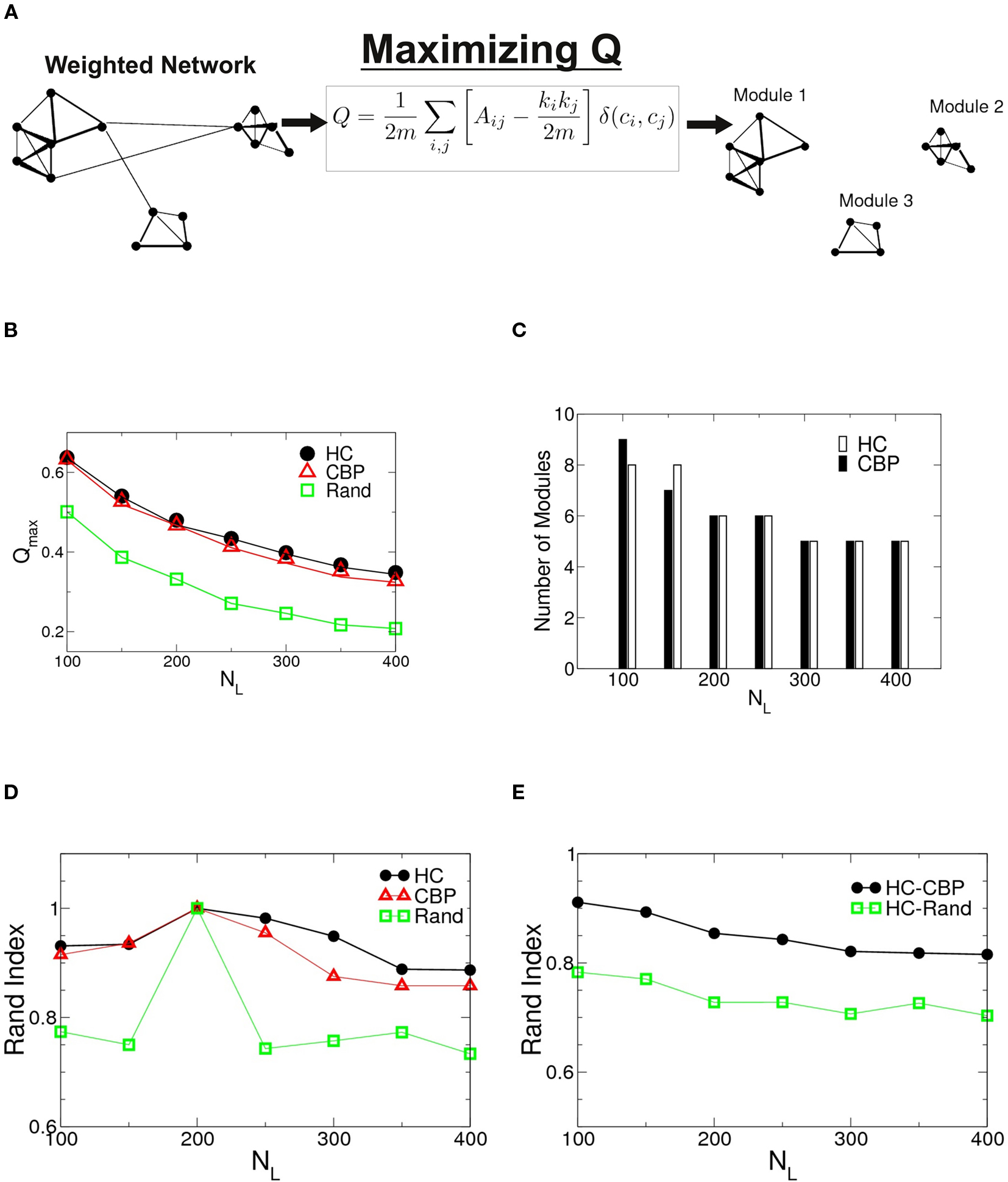
Figure 2. (A) Schematic representation of the algorithm to find modularity (Eq. 5) identifying nodes mutually connected more strongly than with the rest of the network. (B) Changes in the maximum modularity as a function of the number of links, N_L for both groups as well as for an equivalent random network. (C) Number of modules at Q_max as a function of N_L for both groups. (D) Robustness of the communities structures. Rand index of partitions obtained for different values of N_L = {100,150,250,350,400} compared with those of N_L = 200 for HC (black circles), CBP (red triangles), and equivalent random weighted networks (green squares). (E) Rand index between partitions of HC and CBP (black circles) as a measure of module’s similarity in both groups. The Rand index is also calculated between HC and equivalent random weighted networks (green squares). The difference between both groups community’ structures is smaller than the difference expected between HC and an equivalent random network.

To further investigate possible differences between groups, the sets of modules found at Q_max were compared, using the Rand index (RI) (Rand, 1971). The RI is a coefficient that quantifies the percentage of agreement between two partitions (X and Y) of a given set of elements. Thus, RI = 1 if both partitions X and Y are exactly the same (i.e., they have the same quantity of modules and the same integrants en each one) and RI = 0 if they are completely different.

In Figure 2D we shown the calculated RI between networks of different N_L with the one corresponding to N_L = 200 for HC, CBP, and a random realization. No major changes in community organization for brain networks is observed as a function of N_L, but large changes are shown in equivalent random networks. This result suggest that the observed structures are a robust feature of the brain networks.

Figure 2E shows the RI between HC and CBP partitions (black circles) as a function of N_L, with the RI calculated between HC and a random equivalent network (green diamond). The differences found between HC and CBP are much smaller than those expected between HC and equivalent random networks. These results suggest that more detailed analysis is needed to identify potential differences between control subjects and patients. In order to do this we will restrict further analysis to networks with a fixed N_L. Since the number of communities at Q_max stabilizes for N_L = 200, such value was chosen as representative.

The modular structure in which the brain network organizes (for N_L = 200) are shown in Figure 3 depicted in two ways. In the left panels we use an anatomical representation with the coordinates of the center of mass of each region. Right panels display a brain representation in axial, coronal, and sagittal views of found communities over a MNI-152 template atlas. We can observe that both, the HC and the CBP group networks, show a structure formed by up to six communities which are listed in Table A2, along with the membership for each community (see Appendix). Abbreviations used for brain regions (as in Salvador et al., 2005) can be found in Table A1 (see Appendix).

FIGURE 3

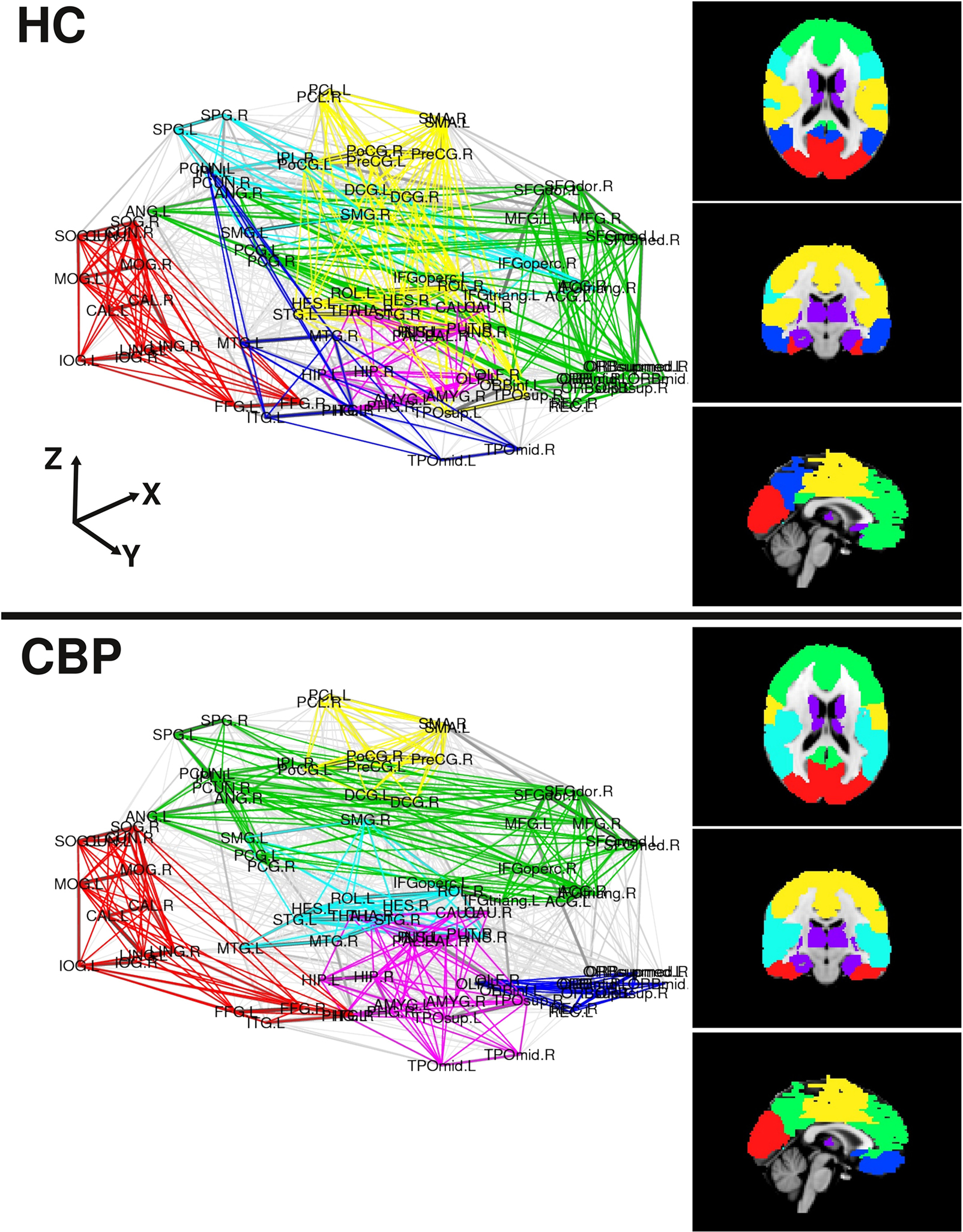
Figure 3. Community organization for both group networks in two representations. Left panels use the coordinates of the center of mass of each region, the right panels depict axial, coronal and sagittal views of the found communities over a MNI-152 template atlas. Modules are colored as listed in Table A2 (see Appendix).

A detailed analysis of these findings can be summarized as follows (see also Figure A1 in Appendix): The first community (red/visual) involves several regions of the lateral and medial visual pathways (calcarine, cuneus, lingual, and occipital gyrus) and could be related to the visual resting state network postulated by Beckmann et al. (2005). This community appears to extend to the inferior temporal gyrus in CBP, but not in HC. A second community (green/fronto-medial) was mainly composed of several frontal regions (superior and inferior frontal gyrus, orbito-frontal cortex), as well as anterior cingulate and angular gyri. This community could be related to two resting state networks: the default mode (DMN) and the executive control networks (Beckmann et al., 2005). This community appears to be altered in CBP patients, because it extends to the precuneus and the medial frontal cortex in CBP patients, but does not include the orbito-frontal cortex as it occurs in HC. The third community (blue/parieto-temporal) is formed by the precuneus and the temporal lobes in HC, displaying similarities to Beckmann’s DMN. This community extends to the orbito-frontal cortex in CBP patients, but not in HC. The fourth community (light blue/fronto-parietal) involves regions from the inferior frontal cortex, the superior parietal and the supramarginal gyrus, and could be associated with two resting state networks: the auditory system and the dorsal visual stream (Beckmann et al., 2005). This community extends to the insula in CBP patients, but not in HC. The fifth community (magenta/subcortical) is comprised by subcortical regions, such as hippocampus, thalamus, basal ganglia, and amygdala. No differences between groups appeared in the module membership of this community. The last community (yellow/sensorimotor) includes the sensorimotor cortices as well as other regions of the pain network such as cingulate gyrus and insula (Zaki et al., 2007). This community appears to be altered in CBP patients because it does not include the insula and the posterior portion of the cingulate gyrus as it occurs in HC. A side by side comparison between HC and CBP communities and Beckmann’s resting state networks can be found in Figure A1 of Appendix.

B. Pairwise Correlations Suffice to Explain Communities Changes?

The results displayed in Figure 3 show that the observed changes in modular organization are basically of three types: (I) there are communities that split into two or more subgroups, (II) there are modules that fuse together forming a single community, and (III) nodes are adsorbed into other communities, and some communities disappear. Admitting that these changes can be brought about by a complex combination of factors, we test here for the simplest of all cases, which is that linear bivariate correlation changes can be sufficient to explain any of the three types of communities changes.

Thus we re-analyze the interactions between nodes through pairwise correlations. An important point is that we start taking the community partition of the HC (Figure 3 top) as a reference frame and compute the mean intra-modular correlation, , for each of the communities defined in this reference HC group. The idea is that should estimate the strength of the bonds holding together the communities, and that changes should occurs preferentially in weakly coupled modules. Figure 4A shows for each of the six communities in both groups. It can be seen that CBP patients exhibit a mean intra-modular correlation smaller that control subjects, with the exception of the posterior module (red). This is consistent with the expectation that communities with weakest correlations should be the ones more easily segregated by potential pathological changes in the interactions.

FIGURE 4

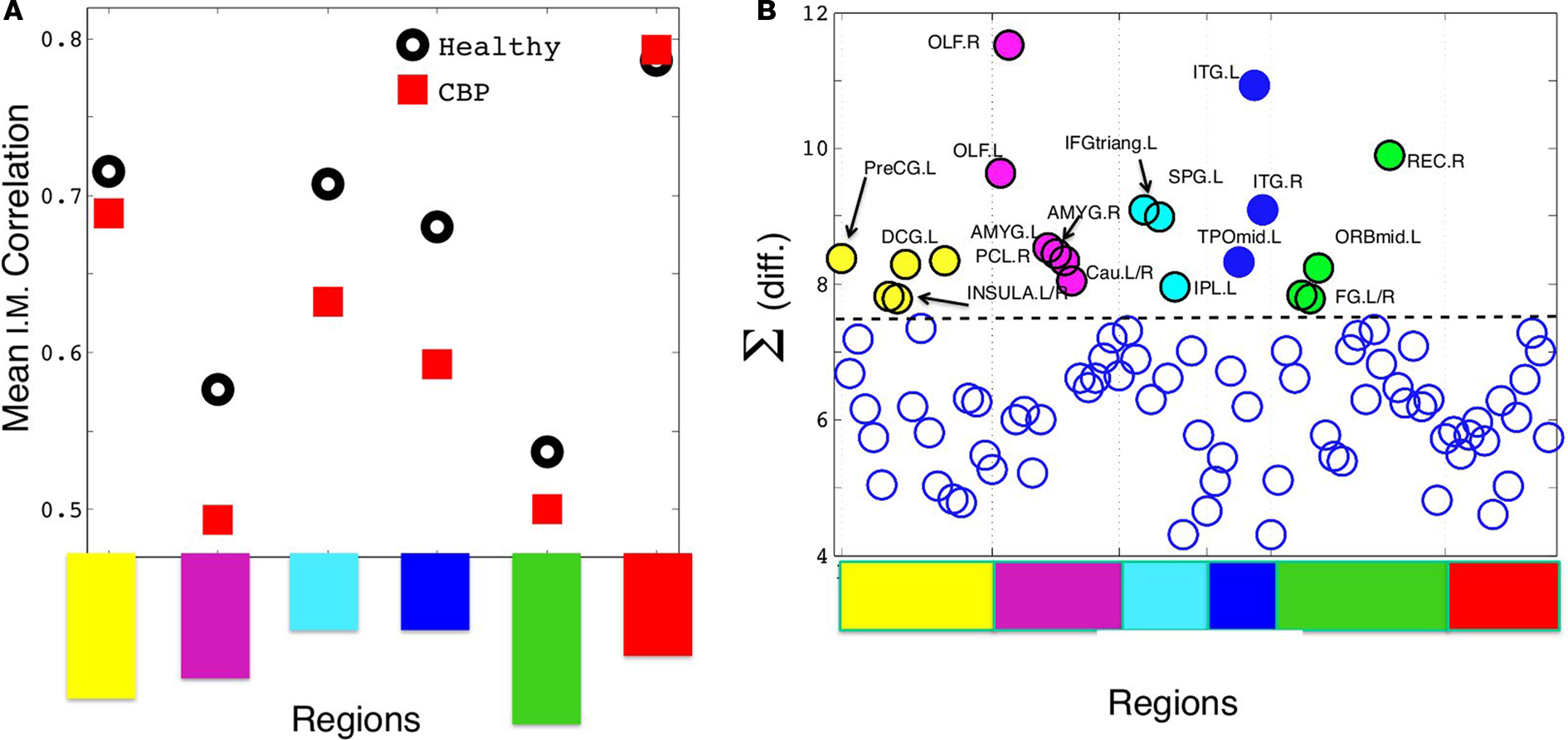
Figure 4. (A) Mean intra-modular correlation for both groups. Notice that, with one exception, all CBP modules show weaker correlations than the corresponding HC communities. (B) The summatory of the HC–CBP absolute differences in pairwise correlation computed for each brain region. Regions with the biggest changes (labeled), hold the key to understand the community changes. Communities labeled with the same colors as in Figures 1C and 3; Table.

Thus we focus at the weight (interaction) changes within each community. The largest changes respect to the HC hold the key to understand all the community alterations. We start by computing the summatory of correlations for each node (plotted in Figure 4B) and inspecting the nodes exhibiting the largest (absolute) change in its correlations. Then, we look whether these changes can explain directly any of the structural changes observed in a given community.

The corresponding observed changes, as listed below (see Figure 5):

FIGURE 5

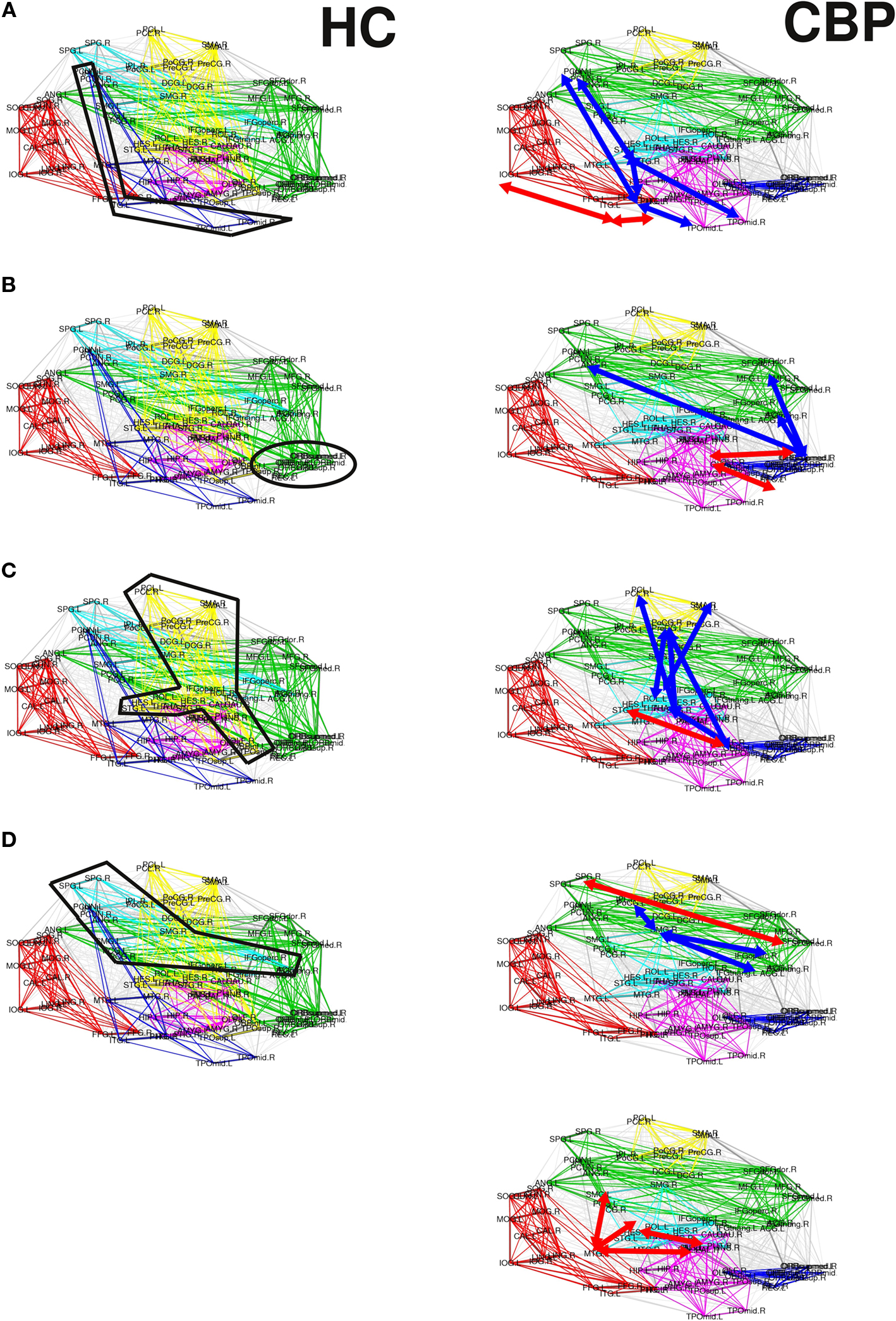
Figure 5. Summary of the alterations in pairwise correlations driving the observed changes in the reorganization of the CBP networks. HC and CBP partitions are shown in left and right columns respectively. Changes associated with the parieto-temporal, fronto-medial, and sensorimotor communities are shown in (A) (B) and (C) respectively. Variations in the fronto-parietal community are shown in (D) and (E). Interactions strengthened in CBP patients respect to the HC group are indicated by red arrows, while those weakened are denoted with blue arrows.

(a) The parieto-temporal community (Coded blue in HC, Figure 5A) is not present in CBP. In this module all the pair correlations have decreased (range [−0.2,−0.1]) in CBP, breaking this structure apart. Larger correlation levels observed in CBP than in HC between inferior temporal gyrus (ITG) and lingual (LING), fusiform (FFG), and inferior occipital gyrus (IOG) (+0.15) result in the former (ITG) being included in the posterior community (red).

(b) The fronto-medial (green) community observed in HC splits in two subgroups: a new CBP (orbito-frontal, blue) community is created and the fronto-medial CBP community (green) is reorganized, (see Figure 5B). These changes can be explain by the increased interaction between olfactory (OLF), the orbital part of the superior frontal gyrus (ORBsup) and the gyrus rectum (REC) (+0.16) in CBP. Simultaneously the correlation between the orbital part of the middle frontal gyrus (ORBmid) and angular (ANG), middle frontal (MFG), and anterior cingulate gyrus (ACG) decreased (−0.12). This two opposite behaviors give raise to a mean intra-modular correlation that do not change considerably in CBP.

(c) The same type of behavior can be observed for the Sensorimotor HC community (yellow, Figure 5C). In this case, the interaction between the insula and the precentral gyrus (PreCG), the paracentral lobule (PCL), and superior temporal gyrus of temporal pole (TPOsup) are lower in CBP than in HC (−0.13). In addition, the interactions between rolandic operculum, supplementary motor area (SMA) and precentral gyrus (PreCG) are decreased (−0.12), whether correlations between insula and Heschl gyrus in CBP are increased (+0.11).

(d) The fronto-parietal (light-blue) community observed in HC is adsorbed by the fronto-medial module in CBP (Figure 5D), mainly because the interaction between superior parietal (SPG) and supramarginal (SMG) has increased (+0.15).

(e) In addition, the supramarginal (SMG) region is left apart from the fronto-parietal HC module in CBP (Figure 5E). This happens because the interaction between this and inferior parietal (IPL), the opercular part of the middle frontal gyrus (IFGoperc) and the triangular part of the inferior frontal gyrus (IFGtriang) is decreased (−0.14). In this case all the regions involved in the new community have increased their internal interactions (superior temporal, supramarginal and middle temporal gyrus, insula, and Heschl operculum).

The mentioned arguments show that the changes observed in the CBP networks can be explained by looking at the pairwise interaction changes within each community and focusing on the largest correlation changes respect to the HC. At some point this is to be expected as the algorithm uses precisely these correlations when it assign each node to a given community.

C. Hubs and Connectors

The results discussed in the previous section show that both CBP and HC networks are structured in the same number of communities, although they show notorious differences in organization and region’s membership. This produces that, within these communities, certain key regions present different connectivity. To further quantify these differences, the z-score of the intra-modular degree (z_i) and the participation coefficient (P_i) of each node were computed (e.g., Eqs. 6 and 7). This technique allows the labeling in each case of hubs and connectors for each module as it is presented in the top panels of Figure 6 (see names for each region further detailed in Table 1).

FIGURE 6

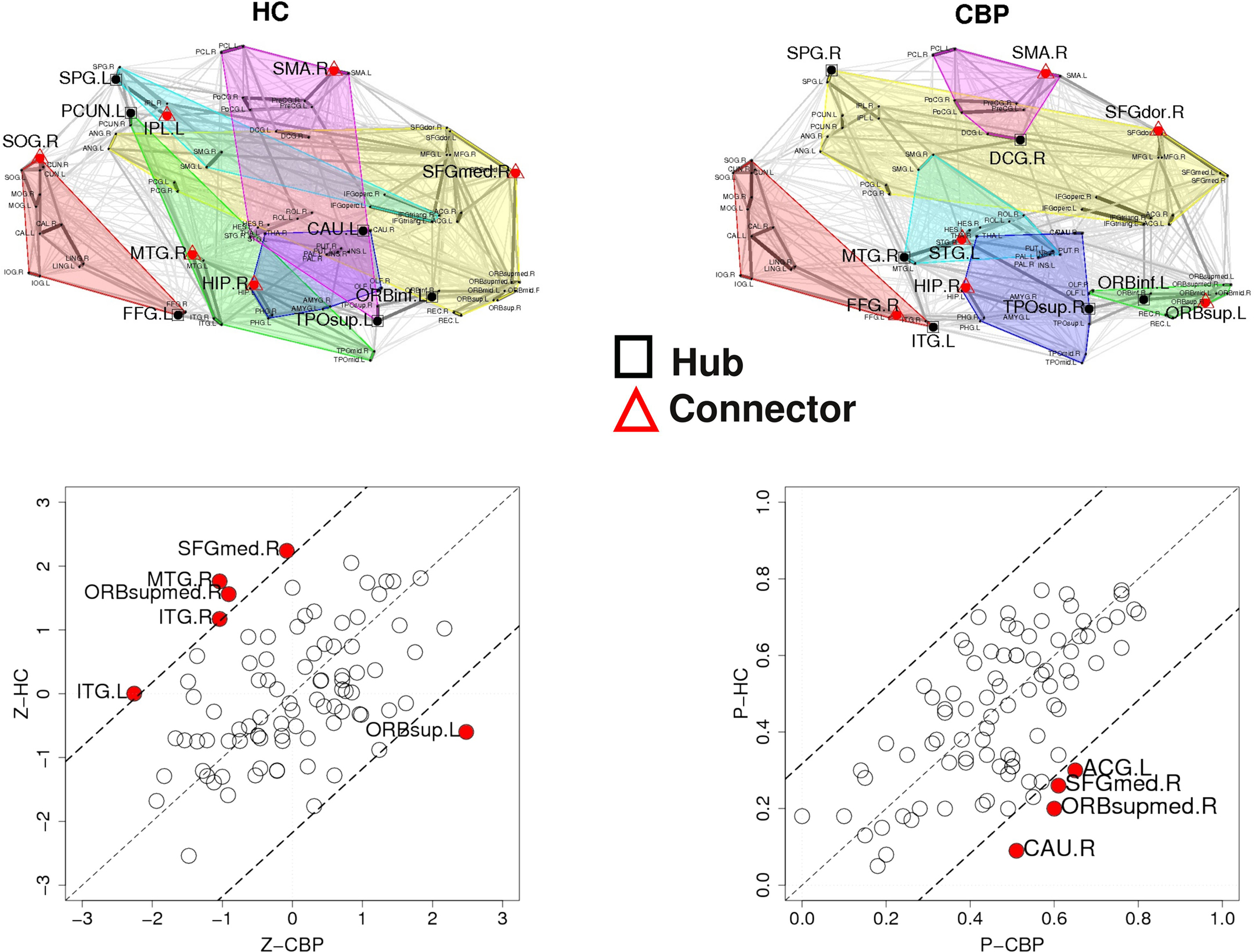
Figure 6. Top panels: Hubs (nodes with highest intra-modular degree) and connectors (highest participation coefficient) in each module for both group networks. Bottom panels: Left: versus , right versus . The regions which display a role’s change larger than two standard deviations (dashed lines) are labeled and plotted using filled circles.

TABLE 1

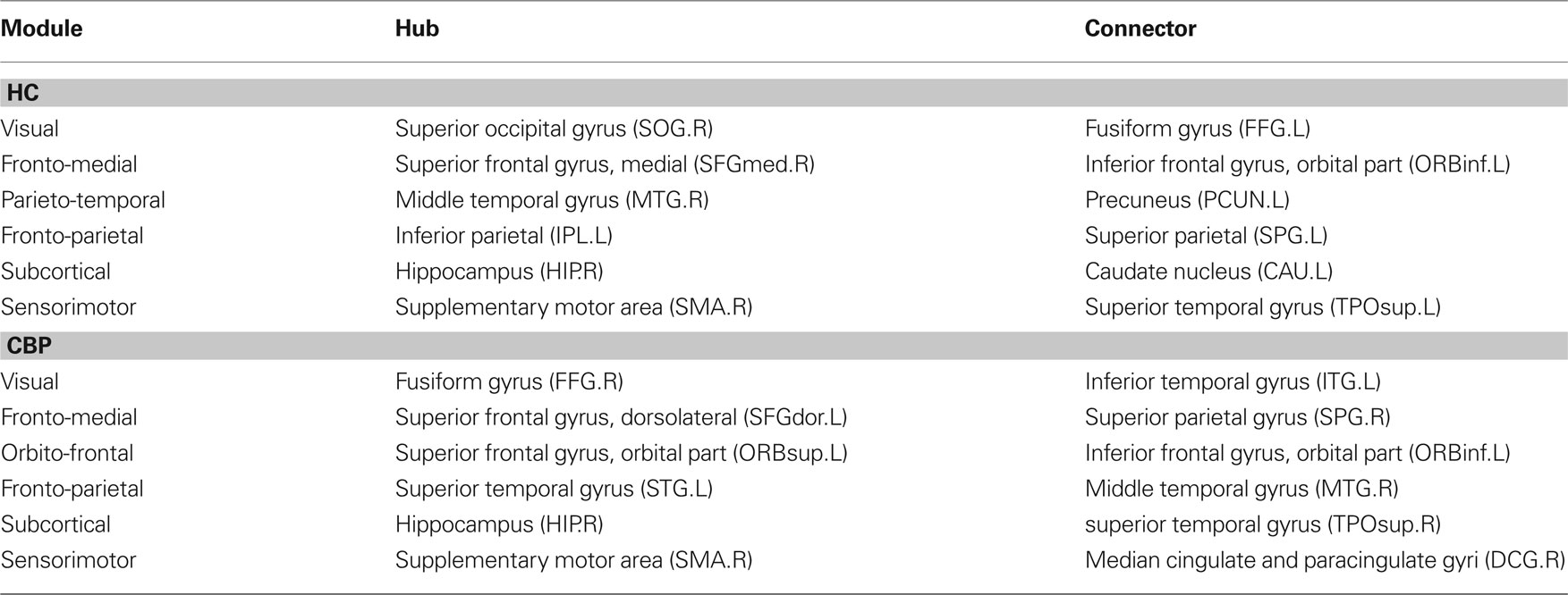
Table 1. Rregions identified as hubs or connectors for each of the communities in both groups.

The location of hubs and connectors provide clues about the key players in each module organization, thus it is important to study the changes in role of these nodes between the groups. This is plotted in the bottom panels of Figure 6 for the intra-modular degree and participation coefficient of healthy controls and versus chronic back pain patients, and . If there were no changes in z_i and P_i, all points should collapse in the diagonal, thus, distance from the diagonal can be interpreted as a measure of region’s role change. In the plot, those regions whose change in z_i or P_i are more than two standard deviations are highlighted. Concerning hubs, note that inferior temporal gyrus (ITG.L and ITG.R), superior frontal gyrus, medial orbital (ORBSupMed.R), middle temporal gyrus (MTG.R) and superior frontal gyrus, medial (SFGmed.R) are regions with high intra-modular degree in HC and low intra-modular degree in CBP patients. Superior frontal gyrus, orbital part (OrbSup.L) is a region with high intra-modular degree in CBP and low in HC. Concerning connectors, caudate (CAU.R), superior frontal gyrus, medial orbital (ORBSupMed.R), superior frontal gyrus, medial (SFGmed.R) and anterior cingulate, and paracingulate gyri (ACG.L) are regions whose participation coefficient increase notoriously in CBP respect to HC groups.

For any given node, changes in its z_i or P_i value could arise basically due to two mechanisms: local changes, i.e., when there are changes in its own connectivities (by increasing or decreasing the number of links with the rest of the network) or global changes, i.e., due to changes in the mean intra-modular degree by alterations in other connections or by a change in module memberships. These is demonstrated by the results in Table 2 which shows the degree of these regions and compare with <k_i> of regions who belong to.

TABLE 2

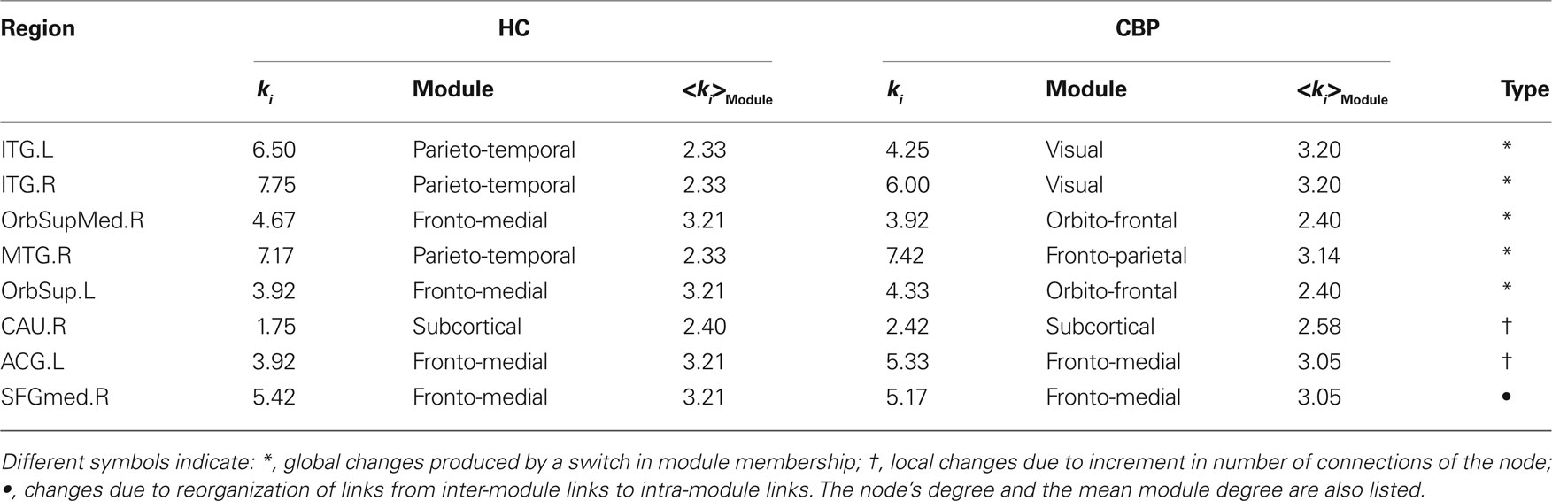
Table 2. Changes in node's role.

IV. Discussion

The major aim of the present study was to examine the modular organization of functional brain networks in CBP. To characterize the modularity of these complex networks, we applied tools from graph theory to BOLD time series obtained from resting fMRI. The present findings were derived from purely data driven analyses and confirmed by a heuristic approach using pairwise correlations. Based on previous evidence showing extensive alterations of brain dynamics in chronic pain patients (Baliki et al., 2006, 2008; Geha et al., 2008; Tagliazucchi et al., 2010), we hypothesized that topological properties of these functional brain networks (i.e., number and components of the modules, intra-modular degree, participation coefficient of the nodes) should be altered as a consequence of persistent pain. Our results revealed significant group differences in the modular organization of several brain resting state networks, rather than global changes of brain modularity. Basically, we observed that HC and CBP patients differed in the connectivity of frontal lobes and anterior cingulate gyrus, which are usually involved in the default mode resting state network and pain processing. To our knowledge, this is the first report analyzing in detail the structure of these functional brain networks in CBP patients. Indeed, we found that functional brain networks in both healthy and CBP patients were well described by six different communities of modules: Visual (com1), fronto-medial (com2), parieto-temporal (com3), fronto-parietal (com4), subcortical (com5), and sensorimotor (com6). Moreover, it was observed that the modular organization of the functional brain networks in HC was in line with previous studies (Meunier et al., 2009a,b), describing a posterior community (similar to our visual community), a central community (including the sensorimotor and the subcortical communities), and an additional community involving frontal and cingulate cortices as well as the temporal lobes (similar to our fronto-medial and parieto-temporal communities). As a further validation of our approach, we demonstrated that our visual, fronto-medial, parieto-temporal, and fronto-parietal communities were quite similar to the visual, default mode, executive control, and auditory resting state networks (Beckmann et al., 2005), respectively.

Differences between healthy subjects and CBP patients were mainly characterized by a reorganization of fronto-medial, parieto-temporal, fronto-parietal, and sensorimotor communities i nvolving frontal and temporal structures, as well as sensorimotor cortex, basal ganglia, insula, and anterior cingulate cortex (ACC). Basically, this reorganization implied a change in the module membership of the orbito-frontal cortex, the insula, and the posterior portion of the cingulate gyrus, which are involved in affective and cognitive processing, as well as in somatosensory integration. In addition, we found that caudate nucleus and ACC displayed a high inter-modular connectivity in CBP patients as compared with HC. The ACC has been identified as a key brain region in pain processing, responsible for the integration of sensory, attentional, emotional, and motivational aspects of pain; whereas the caudate nucleus participates in pain processing in sync with the ACC and several regions of the prefrontal cortex (Oshiro et al., 2009). Thus, it appears that chronic pain might be associated with changes in the modular organization and with an increased functional correlation of brain regions involved in processing and integration of sensory, affective, and cognitive components of pain. These findings are consistent with previous reports, showing that enduring pain might disrupt the functional connectivity of cortical regions of the DMN with the insula and the middle frontal gyrus (Baliki et al., 2008; Tagliazucchi et al., 2010), key regions which appear to be implicated in internally generated thought processes (Raichle et al., 2001) and to play an important role in the evaluation of pain intensity and other somatic signals (Critchley et al., 2004). Moreover, it has been reported that irrespective of the location, nature or course of the different pain syndromes, chronic pain patients exhibit significant reductions of gray matter in cingulate cortex, orbito-frontal cortex, and insula (May, 2008). Accordingly, it seems reasonable that persistent, emotionally laden, self-reflective thoughts as it occurs in chronic pain states might have led to disrupt the modular organization of insula and orbito-frontal cortex and to increase the number of connections of ACC with the rest of the brain.

Our results show an organization comprising the same number of modules, and when changes were detected, they were well explained by straightforward pairwise changes in the linear correlation between a few nodes. Although caution should be always exercised, the fact that pairwise correlations were sufficient to explain global changes, suggests that correlations between a small number of key regions have a chance to be informative about the functional brain connectivity. Another implication of the present results relates to the physical substrate sustaining these dynamical changes, in particular since it has been previously described that chronic pain may elicit relevant changes in white and gray matter (Geha et al., 2008; May, 2008). These findings are consistent with the alterations in correlations described here, but further studies are needed to establish the validity and extent of the functional and structural relation. If proven true it will reinforce the idea that the stressful experience of enduring pain over many years could by itself modify adaptive synaptic connections, reshaping the connectivity of the subnetworks studied in the present study.

The present study has several limitations. An important one is the underlying assumption that chronic pain patient’s brain is altered by the disease. Although this is a reasonable hypothesis it is yet far from proven and, in addition, even if there are alterations, still is unknown how large could be the individual variability. In other words, it is not yet known up to which point the potential changes in cortical dynamics in each individual are consistent across the patient’s group, such that it can be detected by the kind of group average analyses performed here. Another important limitation is the common assumption considering the ninety anatomically defined brain areas as representing the centerpieces of a large-scale brain network. This is a good simplifying approach, that facilitates and compresses information, but it could be limiting our ability to detect differences between groups. One of the reasons is that regions selected by this method, despite covering very different sizes of cortical territories are all being equalized when considered as a single node in a network. Finally, another factor to consider is that the components obtained from an anatomical parcellation method do not necessarily mirror the dynamical components of brain activity as is shown in Figures A1 and A2 of Appendix where communities found in this work were compared with networks obtained from principal component analyses (as in Beckmann et al., 2005).

In summary, the study of brain correlation networks revealed an organization of up to six communities with similar modularity in both healthy and chronic pain groups. These differences appeared in the membership of key communities of frontal and temporal regions and confirmed by a surprisingly naive analysis based on pairwise correlations of the strongest and weakest correlated regions in HC. Besides confirming the brain effects of long enduring pain, our results provide a framework for studying the effects of other chronic conditions on functional brain networks.

Conflict of Interest Statement

The authors declare that the research was conducted in the absence of any commercial or financial relationships that could be construed as a potential conflict of interest.

Acknowledgments

The authors thank the patients and the healthy volunteers for their participations in the study. Work supported by NIH NINDS of USA, grant No. NS58661, by CONICET (grant No. PIP0802/10 and PIP0087), MinCyt (Grant No. 863) and University of Buenos Aires (grant No. UBACyT X-404), Argentina and by Spanish Ministry of Science and European Funds FEDER (grant No. SEJ2007-62312). Funding for data collection was provided by grant No. NS35115 (awarded to A.V. Apkarian) by NIH NINDS.

Footnote

1. ^http://www.fmrib.ox.ac.uk/analysis/research/flirt/.

References

Achard, S., and Bullmore, E. T. (2007). Efficiency and cost of economical brain functional networks. PLoS Comput. Biol. e17. doi: 10.1371/ journal.pcbi.0030017.

Pubmed Abstract | Pubmed Full Text | CrossRef Full Text

Ahnert, S. E., Garlaschelli, D., Fink, T. M. A., and Caldarelli, G. (2007). Ensemble approach to the analysis of weighted networks. Phys. Rev. E. 76, 016101–016105.

CrossRef Full Text

Apkarian, A. V., Sosa, Y., Krauss, B. R., Thomas, P. S., Fredrickson, B. E., Levy, R. E., Harden, R., and Chialvo, D. R. (2004). Chronic pain patients are impaired on an emotional decision-making task. Pain 108, 129–136.

Pubmed Abstract | Pubmed Full Text

Baliki, M. N., Chialvo, D. R., Geha, P. Y., Levy, R. M., Harden, R. N., Parrish, T. B., and Apkarian, A. V. (2006). Chronic pain and the emotional brain: specific brain activity associated with spontaneous fluctuations of intensity of chronic back pain. J. Neurosci. 26, 12165–12173.

Pubmed Abstract | Pubmed Full Text | CrossRef Full Text

Baliki, M. N., Geha, P. Y., Apkarian, A. V., and Chialvo, D. R. (2008). Beyond feeling: chronic pain hurts the brain, disrupting the default-mode network dynamics. J. Neurosci. 28, 1398–1403.

Pubmed Abstract | Pubmed Full Text | CrossRef Full Text

Beckmann, C. F., DeLuca, M., Devlin, J. T., and Smith, S. M. (2005). Investigations into resting-state connectivity using independent component analysis. Philos. Trans. R. Soc. Lond. B. Biol. Sci. 360, 1001–1013.

Pubmed Abstract | Pubmed Full Text | CrossRef Full Text

Beckmann, C. F., and Smith, S. M. (2004). Probabilistic independent component analysis for functional magnetic resonance imaging. IEEE Trans. Med. Imag. 23, 137–152.

CrossRef Full Text

Boettcher, S., and Percus, A. G. (2001a). Optimization with extremal dynamics. Phys. Rev. Lett. 86, 5211–5214.

CrossRef Full Text

Boettcher, S., and Percus, A. G. (2001b). Extremal optimization for graph partitioning. Phys. Rev. E. 64, 026114–026126.

CrossRef Full Text

Broyd, S. J., Demanuele, C., Debener, S., Helps, S. K., James, C. J., and Sonuga-Barke, E. J. S. (2009). Default-mode brain dysfunction in menthal disorders: a systematic review. Neurosci. Biobehav. Rev. 33, 279–296.

Pubmed Abstract | Pubmed Full Text | CrossRef Full Text

Bullmore, E. T., and Sporns, O. (2009). Complex brain networks: graph-theoretical analysis of structural and functional systems. Nat. Rev. Neurosci. 10, 186–198.

Pubmed Abstract | Pubmed Full Text | CrossRef Full Text

Clauset, A., Newman, M. E. J., and Moore, C. (2004). Finding community structure in very large networks. Phys. Rev. E. 70, 066111–066116.

CrossRef Full Text

Cordes, D., Haughton, V. M., Arfanakis, K., Carew, J. D., Turski, P. A., Moritz, C. H., Quigley, M. A., and Meyerand, M. E. (2001). Frequencies contributing to functional connectivity in the cerebral cortex in “resting-state” data. Am. J. Neuroradiol. 22, 1326–1333.

Cordes, D., Haughton, V. M., Arfanakis, K., Wendt, G. J., Turski, P. A., Moritz, C. H., Quigley, M. A., and Meyerand, M. E. (2000). Mapping functional related regions of brain with functional connectivity MR imaging. Am. J. Neuroradiol. 21, 1636–1644.

Critchley, H. D., Wiens, S., Rotshtein, P., Ohman, A., and Dolan, R. J. (2004). Neural systems supporting interoceptive awareness. Nat. Neurosci. 7, 189–195.

Pubmed Abstract | Pubmed Full Text | CrossRef Full Text

Damoiseaux, J. S., Rombouts, S. A. R. B., Barkhof, F., Scheltens, P., Stam, C. J., Smith, S. M., and Beckmann, C. F. (2006). Consistent resting-state networks across healthy subjects. Proc. Natl. Acad. Sci. U.S.A. 103, 13848–13853.

Pubmed Abstract | Pubmed Full Text | CrossRef Full Text

Duch, J., and Arenas, A. (2005). Community detection in complex networks using extremal optimization. Phys. Rev. E. 72, 027104–027107.

CrossRef Full Text

Eguiluz, V. M., Chialvo, D. R., Cecchi, G., Baliki, M., and Apkarian, A. V. (2005). Scale-free brain functional networks. Phys. Rev. Lett. 94, 018102–018105.

Pubmed Abstract | Pubmed Full Text | CrossRef Full Text

Fox, M. D., Snyder, A. Z., Vincent, J. L., Corbetta, M., van Essen, D. C., and Raichle, M. E. (2005). From the cover: the human brain is intrinsically organized into dynamic, anticorrelated functional networks. Proc. Natl. Acad. Sci. U.S.A. 102, 9673–9678.

Pubmed Abstract | Pubmed Full Text | CrossRef Full Text

Fox, M. D., and Raichle, M. E. (2007). Spontaneous fluctuations in brain activity observed with functional magnetic resonance imaging. Nat. Rev. Neurosci. 8, 700–711.

Pubmed Abstract | Pubmed Full Text | CrossRef Full Text

Garrity, A. G., Pearlson, G. D., McKiernan, K., Lloyd, D., Kiehl, K. A., and Calhoun, V. D. (2007). Aberrant “default mode” functional connectivity in schizophrenia. Am. J. Psychiatry 164, 450–457.

Pubmed Abstract | Pubmed Full Text | CrossRef Full Text

Geha, P. Y., Baliki, M. N., Harden, R. N., Bauer, W. R., Parrish, T. B., and Apkarian, A. V. (2008). The brain in chronic CRPS pain: abnormal gray-white matter interactions in emotional and autonomic regions. Neuron 60, 570–581.

Pubmed Abstract | Pubmed Full Text | CrossRef Full Text

Guimera, R., and Amaral, L. A. N. (2005). Functional cartography of complex metabolic networks. Nature 433, 895–900.

Pubmed Abstract | Pubmed Full Text | CrossRef Full Text

He, Y., Chen, Z., and Evans, A. (2008). Structural insights into aberrant topological patterns of large-scale cortical networks in Alzheimer’s disease. J. Neurosci. 28, 4756–4766.

Pubmed Abstract | Pubmed Full Text | CrossRef Full Text

Jezzard, P., Mathews, P., and Smith, S. M. (2001). Functional MRI: An Introduction to Methods. Oxford: Oxford University Press.

Laufs, H., Hamandi, K., Salek-Haddadi, A., Kleinschmidt, A., Duncan, J. S., and Lemieux, L. (2007). Temporal lobe interictal epileptic discharges affect cerebral activity in default mode brain regions. Hum. Brain. Mapp. 28, 1023–1032.

Pubmed Abstract | Pubmed Full Text | CrossRef Full Text

Lui, S.,Ouyang, L., Chen, Q., Huang, X., Tang, H., Chen, H., Zhou, D., Kemp, G. J., and Gong, Q. (2008). Differential interictal activity of the precuneus/posterior cingulate cortex revealed by resting state fMRI at 3T in generalized versus partial seizure. J. Magn. Res. Imag. 27, 1214–1220.

CrossRef Full Text

May, A. (2008). Chronic pain may change the structure of the brain. Pain 137, 7–15.

Pubmed Abstract | Pubmed Full Text

Meunier, D., Achard, S., Morcom, A., and Bullmore, E. T. (2009a). Age-related changes in modular organization of human brain functional networks. Neuroimage 44, 715–723.

CrossRef Full Text

Meunier, D., Lambiotte, R., Fornito, A., Ersche, K., and Bullmore, E. T. (2009b). Hierarchical modularity in human brain functional networks. Front. Neuroinform. 3: 37. doi: 10.3389/neuro.11.037.2009.

CrossRef Full Text

Newman, M. E. J. (2004). Analysis of weighted networks. Phys. Rev. E. 70, 056131–056139.

CrossRef Full Text

Newman, M. E. J., and Girvan, M. (2004). Finding and evaluating community structure in networks. Phys. Rev. E. 69, 026113–026127.

CrossRef Full Text

Oshiro, Y., Quevedo, A. S., McHaffie, J. G., Kraft, R. A., and Coghill, R. C. (2009). Brain mechanisms supporting discrimination of sensory features of pain: a new model. J. Neurosci. 29, 14924–14931.

Pubmed Abstract | Pubmed Full Text | CrossRef Full Text

PICA. http://www.fmrib.ox.ac.uk/analysis/research/melodic.

Rand, W. M. (1971). Objective criteria for the evaluation of clustering methods. J. Amer. Stat. Assoc. 66, 846–850.

CrossRef Full Text

Raichle, M. E., MacLeod, A. M., Snyder, A. Z., Powers, W. J., Gusnard, D. A., and Shulman, G. L. (2001). A default mode of brain function. Proc. Natl. Acad. Sci. U.S.A. 98, 676–682.

Pubmed Abstract | Pubmed Full Text | CrossRef Full Text

Salvador, R., Suckling, J., Coleman, M. R., Pickard, J. D., Menon, D., and Bullmore, E. T. (2005). Neurophysiological architecture of functional magnetic resonance images of human brain. Cereb. Cortex 15, 1332–1342.

Pubmed Abstract | Pubmed Full Text | CrossRef Full Text

Smith, S. M., Fox, P. T., Miller, K. L., Glahn, D. C., Fox, P. M., Mackay, C. E., Filippini, N., Watkins, K. E., Toro, R., Laird, A. R., and Beckmann, C.F. (2009). Close correspondence of major functional networks in rest and under task. Proc. Natl. Acad. Sci. U.S.A. 106, 13040–13045.

Pubmed Abstract | Pubmed Full Text | CrossRef Full Text

Soranzo, N., Bianconi, G., and Altafini, C. (2007). Comparing association network algorithms for reverse engineering of large-scale gene regulatory networks: synthetic versus real data. Bioinformatics 23, 1640–1647.

Pubmed Abstract | Pubmed Full Text | CrossRef Full Text

Sporns, O., Chialvo, D. R., Kaiser, M., and Hilgetag, C. C. (2004). Organization, development and function of complex brain networks. Trends Cogn. Sci. 8, 418–425.

Pubmed Abstract | Pubmed Full Text | CrossRef Full Text

Stanberry, L., Murua, A., and Cordes, D. (2008). Functional connectivity mapping using the ferromagnetic Potts spin model. Hum. Brain Mapp. 29, 422–440.

Pubmed Abstract | Pubmed Full Text | CrossRef Full Text

Tagliazucchi, E., Balenzuela, P., Fraiman, D., Chialvo, D. R. (2010). Brain resting state is disrupted in chronic back pain patients. Neurosci. Lett. 485, 26–31.

Pubmed Abstract | Pubmed Full Text | CrossRef Full Text

Tracey, I., and Mantyh, P. W. (2007). The cerebral signature for pain perception and its modulation. Neuron 55, 377–391.

Pubmed Abstract | Pubmed Full Text | CrossRef Full Text

Tzourio-Mazoyer, N., Landeau, B., Papathanassiou, D., Crivello, F., Etard, O., Delcroix, N., Mazoyer, B., and Joliot, M. (2002). Automated anatomical labeling of activations in SPM using a macroscopic anatomical parcellation of the MNI MRI single-subject brain. Neuroimage 15, 273–289.

Pubmed Abstract | Pubmed Full Text | CrossRef Full Text

van den Heuven, M. P., Stam, C. J., Boersma, M., and Hullshof Pol, H. E. (2008). Small-world and scale-free organization of voxel-based resting-state functional connectivity in the human brain. Neuroimage 43, 528–539.

Pubmed Abstract | Pubmed Full Text | CrossRef Full Text

Witting, N., Kupers, R. C., Svensson, P., Jensen, T. S. (2006). A PET activation study of brush-evoked allodynia in patients with nerve injury pain. Pain 120, 145–154.

Pubmed Abstract | Pubmed Full Text

Zaki, J., Ochsner, K. N., Hanelin, J., Wager, T. D., and Mackey, S. C. (2007). Different circuits for different pain: Patterns of functional connectivity reveal distinct networks for processing pain in self and others. Soc. Neurosci. 2, 276–291.

Pubmed Abstract | Pubmed Full Text | CrossRef Full Text