

- Research Institute MOVE, VU University Amsterdam, Amsterdam, Netherlands
In recent studies, functional connectivities have been reported to display characteristics of complex networks that have been suggested to concur with those of the underlying structural, i.e., anatomical, networks. Do functional networks always agree with structural ones? In all generality, this question can be answered with “no”: for instance, a fully synchronized state would imply isotropic homogeneous functional connections irrespective of the “real” underlying structure. A proper inference of structure from function and vice versa requires more than a sole focus on phase synchronization. We show that functional connectivity critically depends on amplitude variations, which implies that, in general, phase patterns should be analyzed in conjunction with the corresponding amplitude. We discuss this issue by comparing the phase synchronization patterns of interconnected Wilson–Cowan models vis-à-vis Kuramoto networks of phase oscillators. For the interconnected Wilson–Cowan models we derive analytically how connectivity between phases explicitly depends on the generating oscillators’ amplitudes. In consequence, the link between neurophysiological studies and computational models always requires the incorporation of the amplitude dynamics. Supplementing synchronization characteristics by amplitude patterns, as captured by, e.g., spectral power in M/EEG recordings, will certainly aid our understanding of the relation between structural and functional organizations in neural networks at large.
Introduction
The interplay between structural and functional brain networks has become a popular topic of research in recent years. It is currently believed that the topologies of structural and functional networks in various empirical systems may disagree (Sporns and Kötter, 2004) but systematic analyses tackling this issue are few and far between. In a combined neural mass and graph theoretical model of electroencephalographic signals, it was found that patterns of functional connectivity are influenced by – but not identical to – those of the corresponding structural level (Ponten et al., 2010). In this and many other studies, functional connectivity has been defined through the synchronization between activities at different nodes.
Neurons synchronize their firing pattern in accordance with different behavioral states. On a larger scale, synchronous activities are considered to stem from meso-scale neural populations that oscillate at certain frequencies with certain amplitudes. That is, oscillatory activity may yield synchronization characteristics within a neural population or between populations (Salenius and Hari, 2003). The amplitude of a single oscillatory neural population reflects the degree of synchronization of its neurons, that is, it measures local synchrony. By contrast, synchronization between two or more oscillatory neural populations is typically defined by their (relative) phase variance. Changes in instantaneous phase locking or coherence reflect changes in more global, distributed synchronization, i.e., between ensembles or between areas. In fact, synchronized activity across neural networks is believed to offer an effective mechanism for information transfer, especially when discriminating between frequency and phase-locked activity (Baker et al., 1999; Mima and Hallett, 1999; Salinas and Sejnowski, 2001; Fries, 2005; Womelsdorf et al., 2007). It is usually assumed that amplitude or power variations take place on long time scales when compared to the phase dynamics and are therefore considered negligible. The coupling that does, or does not, yield synchrony between oscillators hence exclusively depends on the phase. Here we ask whether this assumption is valid, and by this, tackle if a sole focus on phase really covers all functional characteristics of networks. In the present study we describe the dynamics of neural populations at every node as a neural mass model (Wilson and Cowan, 1972; Lopes Da Silva et al., 1974, 1976; Freeman, 1975; Lopes Da Silva, 1991; Jansen and Rit, 1995; Deco et al., 2008) that can behave like weakly coupled self-sustained non-linear oscillators. This description generally allows for deducing the corresponding phase dynamics (Schuster and Wagner, 1990a,b; Aoyagi, 1995; Tass, 1999) and, by this, to investigate how amplitude affects the phase dynamics in neural networks. The phase dynamics is indeed influenced by the amplitudes of the individual oscillators as we show analytically.
In a nutshell, we start off with a network of N Wilson–Cowan neural mass models (Wilson and Cowan, 1972) that are each located at network nodes k = 1, 2, …, N and linked solely through excitatory connections. Every model displays self-sustained oscillations with slightly different natural frequencies. Given a certain structural connectivity between the oscillators denoted by Ckl, we discuss how the connectivity Dkl between phases explicitly depends on the oscillators amplitudes Rk. The expression Dkl ∝ (Rl/Rk)Ckl can be derived analytically by characterizing every oscillator via its amplitude and phase and formulating for the latter the dynamics in terms of a Kuramoto network (Kuramoto, 1984; Strogatz, 2000; Acebron et al., 2005).
The discussed structural connectivities differ qualitatively in their topology. In detail, we consider the fully connected isotropic network, a network with small-world topology generated by the Watts–Strogatz model (Watts and Strogatz, 1998), and an anatomical network reported by Hagmann et al. (2008). Capitalizing on the derived analytical expression for Dkl, we show how the amplitude dependency can alter the topology of connectivity in the network of Wilson–Cowan oscillators when reducing them to the Kuramoto-like network of mere phase oscillators. The connectivity at the level of phase dynamics, Dkl, largely prescribes the functional connectivity as quantified by the resulting synchronization patters. We illustrate this numerically using the aforementioned network topologies that are known to influence synchronizability (Watts and Strogatz, 1998; Barahona and Pecora, 2002; Achard and Bullmore, 2007; Brede, 2008).
Materials and Methods
Network Models
To understand the qualitative relationship between macroscopically defined functional networks and the (underlying) structural connectivity, modeling local populations of neurons in terms of averaged properties like their mean voltage and/or firing rates appears very efficient. This mean-field-like approach has a long tradition and is typically referred to as neural mass modeling (Wilson and Cowan, 1972; Lopes Da Silva et al., 1974, 1976; Freeman, 1975; Lopes Da Silva, 1991; Jansen and Rit, 1995; Deco et al., 2008). Neural mass models have been used to study the origin of alpha rhythm, evoked potentials, pathological brain rhythms, and the transition between normal and epileptic activity (Lopes Da Silva et al., 1974; Jansen and Rit, 1995; Stam et al., 1999a,b; Valdes et al., 1999; David et al., 2005). Several studies considered small networks of two or three interconnected neural mass models (Van Rotterdam et al., 1982; Schuster and Wagner, 1990a,b; Wendling et al., 2001; David and Friston, 2003; Ursino et al., 2007) as well as larger networks of interconnected models (Sotero et al., 2007; Ponten et al., 2010).
Here we chose for Wilson–Cowan as seminal neural mass model because it can readily be derived from microscopic descriptions like integrate-and-fire neurons, but also from more general models like Haken (2002) pulse-coupled neurons. By the same token, the Wilson–Cowan model provides a comprehensive link toward an even more macroscopic description as its continuum limit resembles by now well-established neural field equations (Jirsa and Haken, 1996). That is, Wilson–Cowan units may be viewed as an intermediate but in some sense generic description of densely connected neural populations.
Network of Wilson–Cowan models
As said, we are going to put individual Wilson–Cowan models at every node k of the network under study. Every model contains distinct populations of excitatory and inhibitory neurons that are described by their firing rates. If en denotes the firing rate of an excitatory neuron and in the firing rate of an inhibitory neuron, then a neural mass description can be obtained by averaging over the neural population in terms of  and,
and,  where Ne and Ni are the numbers of excitatory and inhibitory neurons. By this averaging, E and I represent the mean firing rates of all excitatory and inhibitory neurons, respectively, of the neural population in question, i.e., that at node k.
Within that population, every neuron receives input from all other neurons of the population. Furthermore, the excitatory units individually receive constant external inputs pn, whose average is given by  . The sum of all inputs is (instantaneously) integrated in time when it exceeds some threshold θ. This thresholding is realized by means of a sigmoid function S. Without loss of generality we here chose S[x] = (1 + e−x)−1; we note that, in general, the thresholds may differ between excitatory and inhibitory units1. In consequence, the mean firing rates of the neural populations can be cast in the following dynamical system
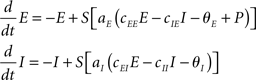
The characteristics of this dynamical system range from a mere fixed-point relaxation to limit cycle oscillations (self-sustained oscillations) depending on parameter settings (Wilson and Cowan, 1972), in particular on the choice of the external input P. That input is usually chosen at random. In the current study, we restrict all parameter values to the regime within which the dynamics displays self-sustained oscillations; see Appendix.
To combine Wilson–Cowan models in a network, different populations are now connected via their excitatory units by virtue of the sum of all El in the dynamics of Ek (see Figure 1). The dynamics at node k then becomes
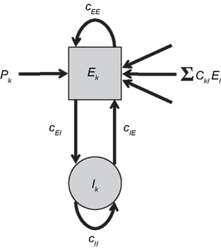
Figure 1. Network of Wilson–Cowan models. At each node k a neural population containing excitatory and inhibitory units (Ek and Ik, respectively) yields self-sustained oscillations. Other nodes are connected to the excitatory unit by means of ΣCklEl. Note that this (mean-field) coupling is scaled by a scalar η – see Eq. 1 for details.
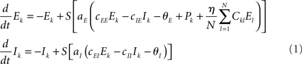
In words, all Wilson–Cowan oscillators, located at nodes l in the network drive the change of the firing rate of the excitatory units Ek. The connectivity is given by the real-valued matrix Ckl that has vanishing diagonal elements, i.e., Ckk = 0. That connectivity matrix is scaled via the overall coupling strength η. It is important to note that the Ckl connectivity matrix is here always identified as the structural connectivity.
As the different Wilson–Cowan models display self-sustained oscillations, it seems obvious to describe them using their amplitude and phase dynamics. The required transforms and approximations are summarized in the Appendix and the outcomes reveal a phase dynamics similar to the seminal Kuramoto network of phase oscillators. The Kuramoto model and its link to the here-discussed network of Wilson–Cowan models will be briefly sketched in the following two sub-sections.
Kuramoto network of phase oscillators
The collective behavior of a network of oscillators, whose states are captured by a single scalar phase φk each, can, in first approximation, be represented by the set of N coupled differential Eq.

That is, the k-th oscillator, with natural frequency ωk, adjusts its phase according to input from other oscillators through a pair-wise phase interaction function sin(φl – φk). The connectivity matrix Dkl is again scaled by an overall coupling strength, η. As will be sketched below, η serves as a bifurcation parameter in that small values of η yield a network behavior that essentially agrees with the entirely uncoupled case (i.e., the phases are not synchronized), whereas η larger than a certain critical value ηc causes the phases to synchronize. The frequencies ωk are distributed according to a specified probability density usually taken to be a symmetric, unimodal distribution (e.g., Lorentzian or Gaussian distributions) with mean ω0. Although the sinusoidal interaction function is an approximation, it still permits a variety of highly non-trivial solutions. As such the model (2) can be viewed as the canonical form for synchronization in extended, oscillatory media. We note that the connectivity matrix Dkl represents also a structural connectivity that does not necessarily agree with that of the Wilson–Cowan model – see below.
Strictly speaking the system (2) does not represent the Kuramoto model in its original form as there the coupling between nodes k and l was considered isotropic and homogeneous, i.e., Dkl = 1 for all connections, by which the model reduces to

For the sake of legibility, however, we here refer to (2) also as the Kuramoto model.
As mentioned above, the effect of increasing η in the isotropic case is to increase the phase synchrony amongst the oscillators. Suppose the coupling is weak (i.e., smaller than the critical value, or η ≪ ηc, then the oscillators’ phases disperse, whereas for strong coupling η ≫ ηc the oscillators become synchronous, i.e., the phases are locked at fixed differences. In the intermediate case η ≈ ηc, clusters of synchronous oscillators may emerge. However, many other oscillators, whose natural frequencies are at the tails of the distribution, are not locked into a cluster. In other words, as η increases, the interaction functions overcome the dispersion of natural frequencies ωn resulting in a transition from incoherence, to partial and then full synchronization (Acebron et al., 2005; Breakspear et al., 2010).
Linking neural mass models to phase oscillators
When deriving the Kuramoto network from the Wilson–Cowan oscillator network, the major ingredient is to average every oscillator over one cycle when assuming that its amplitude and phase change slowly as compared to the oscillator’s frequency. That is, time-dependent amplitude and phase are fixed, the system is integrated over one period to remove all harmonic oscillations, and, subsequently, amplitude and phase are again considered to be time-dependent (Guckenheimer and Holmes, 1990) – this procedure is also referred to as a combination of rotating wave approximation and slowly varying amplitude approximation (Haken, 1974). As shown in more detail in the Appendix, the phase dynamics of the system (1) can in this way be approximated as
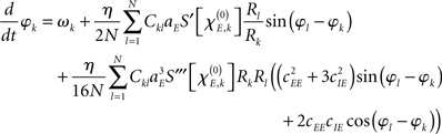
with S′ and S‴ referring to the first and third derivative of the sigmoid function S. The parameter  is given by

with  defining the unstable node within the limit cycle of the Wilson–Cowan model (1) and at network node k. For more details including the definition of the natural frequency we refer to the Appendix. Considering the case that the amplitudes Rk are reasonably small, this phase dynamics can be further simplified to

which does resemble a Kuramoto network. In fact, by comparing this form with the dynamics (2) we find

In sum, the phase dynamics can, in good approximation, be cast into the form of a Kuramoto network provided the connectivity matrix is corrected by means of (3). This correction yields a non-trivial amplitude dependence of the connectivity at the level of the phase dynamics. Since S is a sigmoid function, S′becomes bell-shaped implying a change in connectivity Dkl whenever the parameter  is altered, e.g., by shifting the center of the Wilson–Cowan limit cycle at node k and/or l. This probably more global dependence is supplemented by the here more important node-by-node dependence. When the amplitudes Rk differ per node, the ratio Rl/Rk in (3) directly affects the value of Dkl, which can, strictly speaking, be entirely independent on the choice of the connectivity matrix Ckl. Put differently, the structural connectivity at the neural mass level does not necessarily agree with the structural connectivity at the phase dynamics level.
Given our interest in amplitude dependency, we finally add a note about “large” amplitudes. In line with the Appendix Eq. A.7 including larger amplitudes yields a slight modification of the phase dynamics that we here abbreviate as

Interestingly, the presence of large amplitudes yields, apart from slightly different coupling coefficients  , phase shifts αkl that translate to finite transmission delays. Prior studies that incorporate transmission delays into phase oscillators have revealed elaborate synchronization behaviors (Zanette, 2000; Jeong et al., 2002). The more complex dynamics due to α suggests the notion of frustration, whereby the interaction functions require some finite phase offset in order to vanish (Acebron et al., 2005). For a more detailed discussion we refer to a recent review by Breakspear et al. (2010). Note that for our analytical estimates we always consider the case in which Eq. (2) and (3) apply to good approximation.
Simulations
More recently, several research groups started investigating the relationship between structural and functional connectivity, suggesting that functional connectivity may indeed resemble aspects of structural connectivity, at least to some extent (Lebeau and Whittington, 2005; Ingram et al., 2006; Honey et al., 2007, 2009, 2010; Voss and Schiff, 2009; D’angelo et al., 2010). In most studies, a fixed structural architecture was implemented based on, for instance, the cortical structure of the cat (Zhou et al., 2007), or the macaque neo-cortex (Honey et al., 2007). Yet it is unclear how variations in the network properties at the structural level or fixed network properties with variations by means of (node-dependent) amplitudes may affect the synchronization strength and more global network characteristics at the functional level.
Synchronization was quantified via the phase locking index or the phase uniformity ρ, defined as (Mardia and Jupp, 2000)

This index agrees with the so-called Kuramoto order parameter and reflects the degree of divergence of the different phases in the network (not the relative phases). By varying the overall coupling strength η we induced qualitative differences in synchronization as the order parameter was expected to undergo well-defined bifurcations from an unlocked state to in-phase locking. We simulated both the network of Wilson–Cowan oscillators as well as the Kuramoto network. For the Wilson–Cowan model, we defined the phase as the quadrant-corrected inverse tangents of the ratio of excitatory and inhibitory units at node k, i.e., φk = arctan(Ek/Ik) – this phase largely agreed with the Hilbert-phase of Ek because of the smoothness of the Wilson–Cowan limit cycle. For the Kuramoto network, the phase was, of course, the state variable under study, which did not require any further definition. In all simulations the primary outcome variable in all simulations was, hence, ρ(η) for different network types and, in the case of the Wilson–Cowan network, distinct ranges of input values Pk as will be explained below in all detail. In addition, we computed the phase locking index of the pair-wise relative phases between nodes which served as definition of the functional networks. The precise transform of the Kuramoto network dynamics to the dynamics of relative phases is beyond the scope of the current paper.
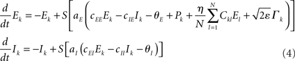
To study potentially “erroneous” simulations of the phase dynamics – and thus possible “misinterpretations” of structural connectivity when solely looking at functional networks defined via phase synchrony – we ignored for the Kuramoto network the amplitude dependency (3) of the connectivity matrix and simply identified Dkl by Ckl. We further accelerated numerical simulations by adding some small dynamic noise (Stratonovich, 1963; Risken, 1989; Daffertshofer, 1998), so-called Langevin forces ⌈ k(t), in the form of mean-centered Gaussian white noise. The simulated dynamics hence looked like
and

Recall that the connectivity in (5) differs from (2) by means of Dkl → Ckl.
Throughout simulations we fixed parameter settings as: aE = 1.2, aI = 2, cEE = 5, cII = 1, cIE = 6, cEI = 10, θE = 2, θI = 3.5. The strength of the dynamical noise was always considered very small (it only served to accelerate numerics and not to discuss impact of stochastic forces). It was set to ε = 10−4 for all simulations of the Wilson–Cowan network (4) and to ε = 10−2 for the Kuramoto network (5). Simulations were realized using a simple Euler-forward scheme with step-size 10−2. Per run a total number of 105 samples were simulated. For each network, simulations were repeated with 10 different realizations of constant but random inputs Pk (Wilson–Cowan oscillators) or constant but random natural frequencies ωn (Kuramoto oscillators). In addition, for the small-world network, new Ckl matrices were generated with different rewiring pattern for each realization. Each of these 10 realizations was again repeated five times with different initial values of Ek and Ik, or φk. The resulting ρ(η) values were computed over the final 100 samples of every run and averaged over all simulations. Primary outcome variable was, hence, ρ(η) for simulations of (4) and (5) using the three different network types, and in the case of the Wilson–Cowan network (4), using altered input-distributions to set Pk.
For the Kuramoto model the natural frequencies ωn were randomly drawn from a Cauchy–Lorentz distribution with width γ = 0.5 and initial φk values at time t = 0 were drawn from a uniform distribution over the interval [0, 2π). The initial Ek and Ik values for the Wilson–Cowan oscillators were uniformly chosen from the interval [0, 1].
By default, the constant input values Pk were drawn from a uniform distribution with −0.25 ≤ Pk ≤ 0.25 for every node k. In order to tackle amplitude effects, however, we looked also at the case in which (selected) nodes displayed oscillations with clearly different amplitudes than others. For this we selected four different intervals from which Pk was drawn: −0.25 ≤ Pk ≤ −0.20; 0.20 ≤ Pk ≤ 0.25; −0.8 ≤ Pk ≤ −0.7; and 0.7 ≤ Pk ≤ 0.8. Simulations were performed using either a single interval or a combination of two intervals for which the first 50% of the nodes were assigned a Pk from the first interval and the second 50% from the second interval. These combinations of intervals were between similar ranges, hence: −0.25 ≤ Pk ≤k −0.20 with 0.20 ≤ Pk ≤ 0.25 and −0.8 ≤ Pk ≤ −0.7 with 0.7 ≤ Pk ≤ 0.8. As shown in the final part of the Appendix the stationary amplitude at network node k either vanishes, i.e., Rk, stationary = 0 or it obeys the form

that by virtue of  explicitly depends on the input Pk. Given this dependency, varying the input Pk systematically could be used to create different scenarios of amplitude effects, which – in particular if selected nodes received significantly different input than others – potentially caused pronounced, qualitative differences between Ckl and Dkl. In these cases, the simulations of (4) and (5) were expected to disagree.
The connectivity matrices Ckl were chosen as either a fully connected isotropic network, as a network with small-world topology generated by the Watts–Strogatz model (Watts and Strogatz, 1998), or via an anatomical network reported by Hagmann et al. (2008). For all the connectivities we estimated the functional networks via phase locking between nodes.
Fully connected homogeneous network
The original Kuramoto network comprises a fully connected homogeneous network – see above. Ckl in this case consists of an N × N matrix containing ones everywhere except for the diagonal, where all values were set to zero, i.e., we did not allow for self-connections. We note that discarding diagonal elements is, strictly speaking, not necessary for the phase dynamics (2) or (6) as the coupling via the sine of relative phase vanishes, i.e., by construction (or symmetry) there are no self-connections. This argument, however, does not apply for the network (1) or (5), hence we always set Ckk = 0.
Although the Kuramoto network is usually studied for large size networks, we chose a network of 66 nodes in order to make a better comparison with the Hagmann dataset.
Small-world network
The model for generating small-world networks employed here was introduced by Watts and Strogatz (1998) to generate graphs with high clustering and low path length (high efficiency). Starting from an ordered network on a ring lattice where nodes are only connected to a small number of direct neighbors, connections are subsequently rewired to a random (distant) node with certain probability. The introduction of a few random connections in an ordered network drastically increases the synchronizability of the network (Watts and Strogatz, 1998; Barahona and Pecora, 2002; Motter et al., 2005; Zhou and Kurths, 2006; Stam and Reijneveld, 2007; Wu et al., 2008; Chen et al., 2009). We used a network with an average degree of 10 and a rewiring probability of 0.2. An example of a Ckl matrix is given in Figure 5 below.
Hagmann network
Empirical networks are unlikely to have an organization that can be exactly described by one of the theoretical network models. To study a network that more realistically represents anatomical connections in the human brain we repeated our simulations on a network that was based on axonal pathways obtained by diffusion spectrum imaging. This dataset has been used to identify the so-called “structural core” of anatomical connections in the human cerebral cortex as described by Hagmann et al. (2008), which is accessible via http://www.connectomeviewer.org/viewer/datasets. To reduce the size of the network and, by this, accelerate simulation time, the original 998 regions were assigned to a 66-node parcellation scheme and averaged over all five subjects as was also done in the original study (Hagmann et al., 2008). The resulting weighted, undirected network was subsequently thresholded to obtain a binary network with an average degree of 10. This network served as our connectivity matrix Ckl; see Figure 2 and also Figure 6 below.
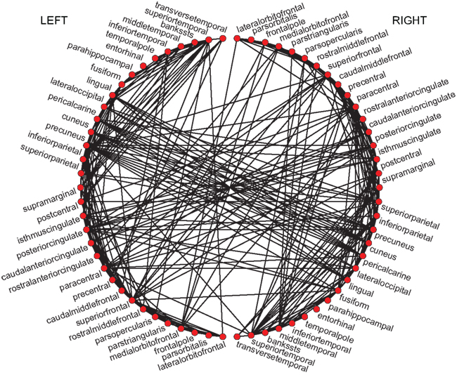
Figure 2. Plot of the Hagmann network (Hagmann et al., 2008). The original 998 regions were assigned to a 66-node parcellation scheme. For the sake of visualization, all 66 nodes are located on the circle; see text for more details.
Results
The changes in synchronization ρ as a function of overall coupling strength η are summarized in Figure 3. First thing to notice is that, for a critical η, the Wilson–Cowan model shows a brisk increase in ρ after which maximal synchronization is reached. Increasing η again after a critical value breaks down the synchronization as the individual Wilson–Cowan oscillators leave the stable limit cycle regime when their inputs exceed a certain value (Schuster and Wagner, 1990a). That means, the neural masses at the different nodes stop oscillating altogether if coupling is too strong. Of course, this does not apply for the Kuramoto model since, by construction, the phases keep oscillating. In consequence, ρ keeps increasing with η and reaches asymptotically maximum synchronization (see bottom row’s panels in Figure 3).
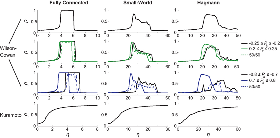
Figure 3. The synchronization ρ as a function of overall coupling strength η for the network of Wilson–Cowan oscillators [Eq. 4; three upper rows] and for the Kuramoto network [Eq. 5; bottom row]. For the upper row, Pk values were drawn from the interval [−0.25,…,0.25], for the second and third row from the indicated intervals (see right-hand side).
The different choices of Pk intervals result in altered synchronization curves. This was most apparent for the [−0.8,…,−0.7] and [0.7,…,0.8] intervals (blue solid lines in Figure 3, third row’s panels) when amplitudes lie furthest apart. In general, different Pk intervals caused a shift in critical η, with networks with larger amplitudes reaching maximum synchronization for lower coupling strength than oscillators with smaller amplitude. Interestingly, the cases with bimodal amplitude distributions (dashed lines) were less synchronizable than their unimodal counterparts. An example of this phenomenon is the case of a fully connected network that reaches global synchronization for each of the [−0.8,…,−0.7] and [0.7,…,0.8] Pk intervals separately but appears unable to fully synchronize for a combination of the two. A closer look at the functional synchronization patterns between individual nodes of this network revealed that two distinct clusters emerged corresponding to the bimodal inputs and thus amplitude distribution (Figure 4).
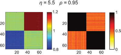
Figure 4. Functional connectivity between the nodes of the fully connected (isotropic and homogeneous) network. Ckl = 1 except for its diagonal elements, Ckk = 0. Input values Pk for the first 33 nodes were drawn from the interval [−0.8,…,−0.7] and the second 33 nodes from the interval [0.7,…,0.8]. Due to this bimodal input distribution, the amplitudes at the nodes and hence their ratios Rl/Rk differ between pairs of nodes (left panel), which yields – by virtue of Eq. (3) – a change in the functional connectivity (right panel). Here it can be seen that the phases of nodes within the same Pk range are fully synchronized but fail to synchronize between clusters; coupling strength was set to η = 5.5 resulting in a global phase synchrony of ρ = 0.95.
If the structural connectivity is isotropic, then amplitude distribution largely (if not fully) prescribes the functional connectivity pattern that thus clearly disagrees with the structural connectivity. In consequence, the current example revealed two strongly synchronized local clusters but the large difference between the input intervals prevented them from synchronizing with one another. It is important to note that, if amplitude effects were not taken into account, a full synchronization of the network would have been found.
With the current parameter settings no full global synchronization could be achieved in both the small-world and the Hagmann network. However, partial synchronization patterns could be observed that did not correspond with the structural connectivity but also not with the distribution of amplitudes (Figures 5 and 6). These patterns rapidly emerged and disappeared with varying η. Although the match with the amplitude distribution was not as clear-cut as in the case of the fully connected network (Figure 4), a similar clustering could be observed, by which the functional connectivities turned out to differ not only quantitatively but also qualitatively from the underlying structural connectivity – a fact that would be missed if relying on a description of sole phase oscillators that show such partial synchronization patterns only in close vicinity of the critical coupling strength.
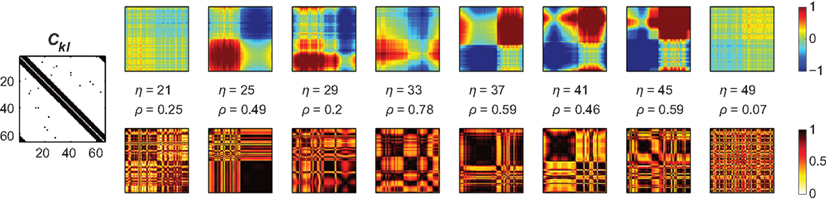
Figure 5. Amplitude ratio distribution [log(Rl/Rk); upper row] and functional connectivity (lower row) of the small-world network that differs from the underlying structural connectivity (Ckl, most left panel). As in Figure 4 we here chose the inputs from a bimodal distribution, here the intervals [−0.8,…,−0.7] and [0.7,…,0.8], which causes the amplitudes to differ between the first and second half of the nodes and, consequently, the functional connectivity matrix to disagree with Ckl. Similar to the homogeneous case in Figure 4 the ratios Rl/Rk largely prescribe the functional connectivity, here, however, mixed with the small-world structure Ckl – see, e.g., the pronounced synchrony along the diagonal that is absent in the patterns of amplitude ratios. In addition, dependent on the overall coupling strength η, pronounced clusters of synchronized nodes appear – the corresponding coupling values, η = 25–45, agree with the synchronization regime of this small-world network displayed in Figure 3, middle column, third row, blue dashed line.
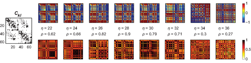
Figure 6. Amplitude ratios [upper row; log(Rl/Rk)] and functional connectivity (lower row) of the Hagmann network using again a bimodal distribution of Pk. The left most panel is again the structural network Ckl; we here used Pk ∈ [−0.25,…,−0.20] and [0.20,…,0.25]. As in the small-world case, localized clusters of synchronized nodes emerge dependent on the overall coupling strength η. These clustered patterns apparently disagree with the underlying anatomical network (most left panel); cf. Figure 3, right column, second row, green dashed lines.
Discussion and Conclusion
The introduction of network analysis to neuroscience has paved new ways for the study of neural network organizations. Particular focus has been on the search for complex networks since many of these networks – especially in the neuroinformatics context – are known for their efficiency when transferring and integrating information from local, specialized brain areas, even when they are distant (Sporns and Zwi, 2004). Over the years, small-world structural networks have been found for C. Elegans (Watts and Strogatz, 1998), cat cortex, and macaque (visual) cortex (Sporns and Zwi, 2004). In humans, anatomical connectivity can be estimated in vivo indirectly via cross-correlation analysis of cortical thickness in structural MRI (He et al., 2007; Chen et al., 2008) and more directly using tractography based on diffusion tensor imaging and diffusion spectrum imaging (Iturria-Medina et al., 2007; Hagmann et al., 2008; Gong et al., 2009). Similar to the structural, i.e. anatomical connections, functional connections have also been found to display characteristics of complex networks, especially by looking at human functional networks in resting state, using either fMRI (Salvador et al., 2005; Achard et al., 2006; Van den Heuvel et al., 2008; Ferrarini et al., 2009) or M/EEG (Stam, 2004; Bassett et al., 2006; Stam and Reijneveld 2007; Bullmore and Sporns, 2009). Changes in these resting state networks appear to relate to neurological and psychiatric diseases like Alzheimer’s disease (Stam et al., 2007, 2009; He et al., 2008; Supekar et al., 2008; de Haan et al., 2009), schizophrenia (Bassett et al., 2008; Liu et al., 2008; Rubinov et al., 2009), ADHD in children (Wang et al., 2009), (removal of) brain tumors (Bartolomei et al., 2006; Bosma et al., 2009), and during epileptic seizures (Kramer et al., 2008; Schindler et al., 2008; Ponten et al., 2009), but also to aging (Achard and Bullmore, 2007; Meunier et al., 2009; Micheloyannis et al., 2009) or to different sleep stages (Ferri et al., 2008; Dimitriadis et al., 2009), as well as during foot movements (De Vico Fallani et al., 2008) and finger tapping (Bassett et al., 2006).
Do these functional networks precisely match their underlying structural counterparts? In general, networks do not agree, especially when the functional networks are solely defined via (phase) synchronization patterns, which is common practice when studying electrophysiological signals, for instance, M/EEG. We have shown that, even if the local dynamics at every node of a network can be described as phase dynamics in the form of a Kuramoto network, the connectivity matrix at this level of phases does not necessarily agree with the connectivity at the level of neural mass models describing firing rates of local neural populations. The connectivity at the phase dynamics level has to be corrected by its amplitude dependency. This phase level is indeed closely related to the empirically assessed functional connectivity matrix as this, as said, is commonly defined through locking patterns of phases. If relying on Kuramoto-like approximations, the connectivity matrix has to be corrected via the relation (3) that may include non-trivial amplitude dependency. Especially, when the amplitudes differ from node to node, the connectivity at the level of phases can qualitatively differ from the structural connectivity at the level of neural mass or mean firing rates. That is, structural and functional connectivity may differ simply because of the latter’s amplitude dependency.
In consequence, phase dynamics and, hence, synchrony patterns should always be analyzed in conjunction with the corresponding amplitude changes. Patterns of global synchrony (phase) may depend on local synchrony (amplitude). This may have profound impacts when linking, for instance, M/EEG studies to neural modeling. Amplitude there translates to (spectral) power, which typically differs between distinct behavioral states or due to pathology. Incorporating these amplitude changes will certainly help to understand how structural and functional network organizations in the cortex, in particular, and in the central nervous system, in general, may relate to one another.
Conflict of Interest Statement
The authors declare that the research was conducted in the absence of any commercial or financial relationships that could be construed as a potential conflict of interest.
Acknowledgments
We thank the Netherlands Organisation for Scientific Research for financial support (NWO grant # 021-002-047).
Footnote
- ^At the individual neuron level, the dynamics reads:
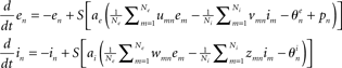
where u, v, w, and z are positive constants representing coupling matrices within the local neural population – see, e.g., Schuster and Wagner(1990a,b) for details.
References
Acebron, J., Bonilla, L., Pérez Vicente, C., Ritort, F., and Spigler, R. (2005). The Kuramoto model: a simple paradigm for synchronization phenomena. Rev. Mod. Phys. 77, 137.
Achard, S., and Bullmore, E. (2007). Efficiency and cost of economical brain functional networks. PLoS Comput. Biol. 3, e174. doi: 10.1371/journal.pcbi.0030017
Achard, S., Salvador, R., Whitcher, B., Suckling, J., and Bullmore, E. (2006). A resilient, low-frequency, small-world human brain functional network with highly connected association cortical hubs. J. Neurosci. 26, 63.
Aoyagi, T. (1995). Network of neural oscillators for retrieving phase information. Phys. Rev. Lett. 74, 4075.
Baker, S. N., Kilner, J. M., Pinches, E. M., and Lemon, R. N. (1999). The role of synchrony and oscillations in the motor output. Exp. Brain Res. 128, 109.
Barahona, M., and Pecora, L. M. (2002). Synchronization in small-world systems. Phys. Rev. Lett. 89, 054101.
Bartolomei, F., Bosma, I., Klein, M., Baayen, J. C., Reijneveld, J. C., Postma, T. J., Heimans, J. J., van Dijk, B. W., de Munck, J. C., de Jongh, A., Cover, K. S., and Stam, C. J. (2006). Disturbed functional connectivity in brain tumour patients: evaluation by graph analysis of synchronization matrices. Clin. Neurophysiol. 117, 2039.
Bassett, D.S., Meyer-Lindenberg, A., Achard, S., Duke, T., and Bullmore, E. (2006). Adaptive reconfiguration of fractal small-world human brain functional networks. Proc. Natl. Acad. Sci. U. S. A. 103, 19518–19523.
Bassett, D. S., Bullmore, E., Verchinski, B. A., Mattay, V. S., Weinberger, D. R., and Meyer-Lindenberg, A. (2008). Hierarchical organization of human cortical networks in health and schizophrenia. J. Neurosci. 28, 9239.
Bosma, I., Reijneveld, J. C., Klein, M., Douw, L., van Dijk, B. W., Heimans, J. J., and Stam, C. J. (2009). Disturbed functional brain networks and neurocognitive function in low-grade glioma patients: a graph theoretical analysis of resting-state MEG. Nonlinear Biomed. Phys. 3, 9.
Breakspear, M., Heitmann, S., and Daffertshofer, A. (2010). Generative models of cortical oscillations: neurobiological implications of the Kuramoto model. Front. Hum. Neurosci. 4:190. doi: 10.3389/fnhum.2010.00190
Brede, M. (2008). Locals vs. global synchronization in networks of non-identical Kuramoto oscillators. Eur. Phys. J. B 62, 87.
Bullmore, E., and Sporns, O. (2009). Complex brain networks: graph theoretical analysis of structural and functional systems. Nat. Rev. Neurosci. 10, 186.
Chen, M., Shang, Y., Zhou, C., Wu, Y., and Kurths, J. (2009). Enhanced synchronizability in scale-free networks. Chaos 19, 013105.
Chen, Z.J., He, Y., Rosa-Neto, P., Germann, J., and Evans, A. C. (2008). Revealing modular architecture of human brain structural networks by using cortical thickness from MRI. Cereb. Cortex 18, 2374.
Daffertshofer, A. (1998). Effects of noise on the phase dynamics of nonlinear oscillators. Phys. Rev. E 58, 327.
D’angelo, E., Mazzarello, P., Prestori, F., Mapelli, J., Solinas, S., Lombardo, P., Cesana, E., Gandolfi, D., and Congi, L. (2010). The cerebellar network: from structure to function and dynamics. Brain Res. Rev. 66, 5.
David, O., and Friston, K. J. (2003). A neural mass model for MEG/EEG: coupling and neuronal dynamics. Neuroimage 20, 1743.
David, O., Harrison, L., and Friston, K. J. (2005). Modeling event-related responses in the brain. Neuroimage 25, 756.
De Haan, W., Pijnenburg, Y. A., Strijers, R. L., van der Made, Y., van der Flier, W. M., Scheltens, P., and Stam, C. J. (2009). Functional neural network analysis in frontotemporal dementia and Alzheimer’s disease using EEG and graph theory. BMC Neurosci. 10, 101. doi: 10.1186/1471-2202-10-101
De Vico Fallani, F., Astolfi, L., Cincotti, F., Mattia, D., Marciani, M. G., Tocci, A., Salinari, S., Witte, H., Hesse, W., Gao, S., Colosimo, A., and Babiloni, F. (2008). Cortical network dynamics during foot movements. Neuroinformatics 6, 23.
Deco, G., Jirsa, V. K., Robinson, P. A., Breakspear, M., and Friston, K. (2008). The dynamic brain: from spiking neurons to neural masses and cortical fields. PLoS Comput. Biol. 4, E1000092. doi: 10.1371/journal.pcbi.1000092
Dimitriadis, S.I., Laskaris, N. A., Del Rio-Portilla, Y., and Koudounis, G. C. H. (2009). Characterizing dynamic functional connectivity across sleep stages from EEG. Brain Topogr. 22, 119.
Ferrarini, L., Veer, I. M., Baerends, E., van Tol, M. J., Renken, R. J., van der Wee, N. J., Veltman, D. J., Aleman, A., Zitman, F. G., Penninx, B. W., van Buchem, M. A., Reiber, J. H., Rombouts, S. A., and Milles, J. (2009). Hierarchical functional modularity in the resting-state human brain. Hum. Brain Mapp. 30, 2220.
Ferri, R., Rundo, F., Bruni, O., Terzano, M. G., and Stam, C. J. (2008). The functional connectivity of different EEG bands moves towards small-world network organization during sleep. Clin. Neurophysiol. 119, 2026.
Fries, P. (2005). A mechanism for cognitive dynamics: neuronal communication through neuronal coherence. Trends Cogn. Sci. 9, 474.
Gong, G., He, Y., Concha, L., Lebel, C., Gross, D.W., Evans, A.C., and Beaulieu, C. (2009). Mapping anatomical connectivity patterns of human cerebral cortex using in vivo diffusion tensor imaging tractography. Cereb. Cortex 19, 524–536.
Guckenheimer, J., and Holmes, P. (1990). Nonlinear Oscillations, Dynamical Systems, and Bifurcations of Vector Fields. New York: Springer.
Hagmann, P., Cammoun, L., Gigandet, X., Meuli, R., Honey, C. J., Wedeen, V. J., and Sporns, O. (2008). Mapping the structural core of human cerebral cortex. PLoS Biol. 6, e159. doi: 10.1371/journal.pbio.0060159
He, Y., Chen, Z., and Evans, A. (2008). Structural insights into aberrant topological patterns of large-scale cortical networks in Alzheimer’s Disease. J. Neurosci. 28, 4756.
He, Y., Chen, Z. J., and Evans, A. C. (2007). Small-world anatomical networks in the human brain revealed by cortical thickness from MRI. Cereb. Cortex 17, 2407.
Honey, C. J., Kötter, R., Breakspear, M., and Sporns, O. (2007). Network structure of cerebral cortex shapes functional connectivity on multiple time scales. Proc. Natl. Acad. Sci. U.S.A. 104, 10240.
Honey, C. J., Sporns, O., Cammoun, L., Gigandet, X., Thiran, J. P., Meuli, R., and Hagmann, P. (2009). Predicting human resting-state functional connectivity from structural connectivity. Proc. Natl. Acad. Sci. U.S.A. 106, 2035.
Honey, C. J., Thivierge, J. P., and Sporns, O. (2010). Can structure predict function in the human brain? Neuroimage 52, 766.
Ingram, P. J., Stumpf, M. P., and Stark, J. (2006). Network motifs: structure does not determine function. BMC Genomics 7, 108. doi: 10.1186/1471-2164-7-108
Iturria-Medina, Y., Canales-Rodríguez, E.J., Melie-García, L., Valdés-Hernández, P.A., Martínez-Montes, E., Alemán-Gómez, Y., and Sánchez-Bornot, J.M. (2007). Characterizing brain anatomical connections using diffusion weighted MRI and graph theory. Neuroimage 36, 645–660.
Jansen, B. H., and Rit, V. G. (1995). Electroencephalogram and visual evoked potential generation in a mathematical model of coupled cortical columns. Biol. Cybern. 73, 357.
Jeong, S. O., Ko, T. W., and Moon, H.T. (2002). Time-delayed spatial patterns in a two-dimensional array of coupled oscillators. Phys. Rev. Lett. 89, 154104.
Jirsa, V. K., and Haken, H. (1996). Field theory of electromagnetic brain activity. Phys. Rev. Lett. 77, 960.
Kramer, M. A., Kolaczyk, E. D., and Kirsch, H. E. (2008). Emergent network topology at seizure onset in humans. Epilepsy Res. 79, 173.
Lebeau, F. E., and Whittington, M. A. (2005). Structure/function correlates of neuronal and network activity – an overview. J. Physiol. 562(Pt 1), 1.
Liu, Y., Liang, M., Zhou, Y., He, Y., Hao, Y., Song, M., Yu, C., Liu, H., Liu, Z., and Jiang, T. (2008). Disrupted small-world networks in schizophrenia. Brain 131, 945.
Lopes Da Silva, F. (1991). Neural mechanisms underlying brain waves: from neural membranes to networks. Electroencephalogr. Clin. Neurophysiol. 79, 81.
Lopes Da Silva, F. H., Smits, H., and Zetterberg, L. H. (1974). Model of brain rhythmic activity. The alpha-rhythm of the thalamus. Kybernetik 15, 27.
Lopes Da Silva, F. H., van Rotterdam, A., Barts, P., van Heusden, E., and Burr, W. (1976). Models of neuronal populations: the basic mechanisms of rhythmicity. Prog. Brain Res. 45, 281.
Meunier, D., Achard, S., Morcom, A., and Bullmore, E. (2009). Age-related changes in modular organization of human brain functional networks. Neuroimage 44, 715.
Micheloyannis, S., Vourkas, M., Tsirka, V., Karakonstantaki, E., Kanatsouli, K., and Stam, C. J. (2009). The influence of ageing on complex brain networks: a graph theoretical analysis. Hum. Brain Mapp. 30, 200.
Mima, T., and Hallett, M. (1999). Corticomuscular coherence: a review. J. Clin. Neurophysiol. 16, 501.
Motter, A. E., Zhou, C., and Kurths, J. (2005). Network synchronization, diffusion, and the paradox of heterogeneity. Phys. Rev. E 71(Pt 2), 016116.
Ponten, S. C., Daffertshofer, A., Hillebrand, A., and Stam, C. J. (2010). The relationship between structural and functional connectivity: graph theoretical analysis of an EEG neural mass model. Neuroimage 52, 985.
Ponten, S.C., Douw, L., Bartolomei, F., Reijneveld, J. C., and Stam, C. J. (2009). Indications for network regularization during absence seizures: weighted and unweighted graph theoretical analyses. Exp. Neurol. 217, 197.
Rubinov, M., Knock, S. A., Stam, C. J., Micheloyannis, S., Harris, A. W., Williams, L. M., and Breakspear, M. (2009). Small-world properties of nonlinear brain activity in schizophrenia. Hum. Brain Mapp. 30, 403.
Salenius, S., and Hari, R. (2003). Synchronous cortical oscillatory activity during motor action. Curr. Opin. Neurobiol. 13, 678.
Salinas, E., and Sejnowski, T. J. (2001). Correlated neuronal activity and the flow of neural information. Nat. Rev. Neurosci. 2, 539.
Salvador, R., Veer, I. M., Baerends, E., van Tol, M. J., Renken, R. J., van der Wee, N. J., Veltman, D. J., Aleman, A., Zitman, F. G., Penninx, B. W., van Buchem, M. A., Reiber, J. H., Rombouts, S. A., and Milles, J. (2005). Neurophysiological architecture of functional magnetic resonance images of human brain. Cereb. Cortex 15, 1332.
Schindler, K.A., Bialonski, S., Horstmann, M. T., Elger, C. E., and Lehnertz, K. (2008). Evolving functional network properties and synchronizability during human epileptic seizures. Chaos 18, 033119.
Schuster, H. G., and Wagner, P. (1990a). A model for neuronal oscillations in the visual cortex. 1. Mean-field theory and derivation of the phase equations. Biol. Cybern. 64, 77.
Schuster, H. G., and Wagner, P. (1990b). A model for neuronal oscillations in the visual cortex. 2. Phase description of the feature dependent synchronization. Biol. Cybern. 64, 83.
Sotero, R. C., Trujillo-Barreto, N. J., Iturria-Medina, Y., Carbonell, F., and Jimenez, J. C. (2007). Realistically coupled neural mass models can generate EEG rhythms. Neural Comput. 19, 478.
Sporns, O., and Kötter, R. (2004). Motifs in brain networks. PLoS Biol. 2, E369. doi: 10.1371/journal.pbio.0020369
Stam, C., de Haan, W., Daffertshofer, A., Jones, B. F., Manshanden, I., van Cappellen van Walsum, A. M., Montez, T., Verbunt, J. P., de Munck, J. C., van Dijk, B. W., Berendse, H. W., and Scheltens, P. (2009). Graph theoretical analysis of magnetoencephalographic functional connectivity in Alzheimers disease. Brain 132, 213.
Stam, C. J. (2004). Functional connectivity patterns of human magnetoencephalographic recordings: a “small-world” network? Neurosci. Lett. 355, 25.
Stam, C. J., Jones, B. F., Nolte, G., Breakspear, M., and Scheltens, P. (2007). Small-world networks and functional connectivity in Alzheimer’s disease. Cereb. Cortex 17, 92.
Stam, C. J., and Reijneveld, J. C. (2007). Graph theoretical analysis of complex networks in the brain. Nonlinear Biomed. Phys. 1, 3.
Stam, C. J., Pijn, J. P., Suffczynski, P., and Lopes da Silva, F. H. (1999a). Dynamics of the human alpha rhythm: evidence for non-linearity? Clin. Neurophysiol. 110, 1801.
Stam, C. J., Vliegen, J. H., and Nicolai, J. (1999b). Investigation of the dynamics underlying periodic complexes in the EEG. Biol. Cybern. 80, 57.
Stratonovich, R. (1963). Topics in the Theory of Random Noise, Vol. I & II. New York, NY: Gordon and Breach.
Strogatz, S. H. (2000). From Kuramoto to crawford: exploring the onset of synchronization in populations of coupled oscillators. Physica D 143, 1.
Supekar, K., Menon, V., Rubin, D., Musen, M., and Greicius, M. D. (2008). Network analysis of intrinsic functional brain connectivity in Alzheimer’s disease. PLoS Comput. Biol. 4, E1000100. doi: 10.1371/journal.pcbi.1000100
Ursino, M., Zavaglia, M., Astolfi, L., and Babiloni, F. (2007). Use of a neural mass model for the analysis of effective connectivity among cortical regions based on high resolution EEG recordings. Biol. Cybern. 96, 351.
Valdes, P. A., Jimenez, J. C., Riera, J., Biscay, R., and Ozaki, T. (1999). Nonlinear EEG analysis based on a neural mass model. Biol. Cybern. 81, 415.
Van Den Heuvel, M. P., Stam, C. J., Boersma, M., and Hulshoff Pol, H. E. (2008). Small-world and scale-free organization of voxel-based resting-state functional connectivity in the human brain. Neuroimage 43, 528.
Van Rotterdam, A., Lopes da Silva, F. H., van den Ende, J., Viergever, M. A., and Hermans, A. J. (1982). A model of the spatial-temporal characteristics of the alpha rhythm. Bull. Math. Biol. 44, 283.
Voss, H. U., and Schiff, N. D. (2009). MRI of neuronal network structure, function, and plasticity. Prog. Brain Res. 175, 483.
Wang, L., Zhu, C., He, Y., Zang, Y., Cao, Q., Zhang, H., Zhong, Q., and Wang, Y. (2009). Altered small-world brain functional networks in children with attention-deficit/hyperactivity disorder. Hum. Brain Mapp. 30, 638.
Watts, D. J., and Strogatz, S. H. (1998). Collective dynamics of “small-world” networks. Nature 393, 440.
Wendling, F., Bartolomei, F., Bellanger, J. J., and Chauvel, P. (2001). Interpretation of interdependencies in epileptic signals using a macroscopic physiological model of the EEG. Clin. Neurophysiol. 112, 1201.
Wilson, H., and R. Cowan, J. D. (1972). Excitatory and inhibitory interactions in localized populations of model neurons. Biophys J. 12, 1.
Womelsdorf, T., Schoffelen, J. M., Oostenveld, R., Singer, W., Desimone, R., Engel, A. K., and Fries, P. (2007). Modulation of neuronal interactions through neuronal synchronization. Science 316, 1609.
Wu, Y., Shang, Y., Chen, M., Zhou, C., and Kurths, J. (2008). Synchronization in small-world networks. Chaos 18, 037111.
Zanette, D. H. (2000). Propagating structures in globally coupled systems with time delays. Phys. Rev. E 62(Pt A), 3167.
Zhou, C., and Kurths, J. (2006). Dynamical weights and enhanced synchronization in adaptive complex networks. Phys. Rev. Lett. 96, 164102.
Keywords: connectivity, phase synchronization, Kuramoto network, Wilson–Cowan model, amplitude dependency
Citation: Daffertshofer A and van Wijk BCM (2011) On the influence of amplitude on the connectivity between phases. Front. Neuroinform. 5:6. doi: 10.3389/fninf.2011.00006
Received: 30 May 2011; Accepted: 20 June 2011;
Published online: 15 July 2011.
Edited by:
Olaf Sporns, Indiana University, USAReviewed by:
Joana R. B. Cabral, Universitat Pompeu Fabra, SpainJuergen Kurths, Humboldt Universität, Germany
Copyright: © 2011 Daffertshofer and van Wijk. This is an open-access article subject to a non-exclusive license between the authors and Frontiers Media SA, which permits use, distribution and reproduction in other forums, provided the original authors and source are credited and other Frontiers conditions are complied with.
*Correspondence: Andreas Daffertshofer, Research Institute MOVE, VU University Amsterdam, Van der Boechorststraat 9, 1081 BT Amsterdam, Netherlands. e-mail:YS5kYWZmZXJ0c2hvZmVyQHZ1Lm5s