 Xiaoguo Yang1†
 Yanyan Zheng
 Chenyang Mei
 Gaoqiang Jiang
 Bihan Tian
 Lei Wang
- 1Wenzhou People’s Hospital, The Third Affiliated Hospital of Shanghai University, Wenzhou, China
- 2School of Ophthalmology and Optometry, Eye Hospital, Wenzhou Medical University, Wenzhou, China
Accurate image segmentation plays a crucial role in computer vision and medical image analysis. In this study, we developed a novel uncertainty guided deep learning strategy (UGLS) to enhance the performance of an existing neural network (i.e., U-Net) in segmenting multiple objects of interest from images with varying modalities. In the developed UGLS, a boundary uncertainty map was introduced for each object based on its coarse segmentation (obtained by the U-Net) and then combined with input images for the fine segmentation of the objects. We validated the developed method by segmenting optic cup (OC) regions from color fundus images and left and right lung regions from Xray images. Experiments on public fundus and Xray image datasets showed that the developed method achieved a average Dice Score (DS) of 0.8791 and a sensitivity (SEN) of 0.8858 for the OC segmentation, and 0.9605, 0.9607, 0.9621, and 0.9668 for the left and right lung segmentation, respectively. Our method significantly improved the segmentation performance of the U-Net, making it comparable or superior to five sophisticated networks (i.e., AU-Net, BiO-Net, AS-Net, Swin-Unet, and TransUNet).
1 Introduction
Image segmentation is an important research direction of computer vision and medical image analysis, and widely used as a preprocessing step for various object detection and disease diagnosis (Khened et al., 2018; Jun et al., 2020). It can divide an image into several disjoint regions by performing a pixel-level classification and largely simplify the assessment of morphological and positional characteristics of object regions (Wang L. et al., 2022; Li et al., 2022). To accurately segment images, a number of image segmentation algorithms have been developed for many different applications, such as threshold based methods (Pare et al., 2019; Shahamat and Saniee Abadeh, 2020), active contour based methods (Han and Graphics, 2006), and random field based methods (Poggi and Ragozini, 1999; Hossain and Reza, 2017). Among these methods, deep learning based methods (Ronneberger et al., 2015; Wang Y. et al., 2022) have gained considerable popularity in the past decade because they can obtain remarkable segmentation performances comparable to manual annotations. Moreover, they are able to automatically extract and flexibly integrate different types of feature information by learning the intrinsic laws and representation levels of images to be segmented.
Despite promising performances, deep learning based methods are often faced with two key challenges in image segmentation (Wang et al., 2021c; Zheng et al., 2022), one is how to obtain rich local information, the other is how to robustly extract high-level semantics. Given the large number of parameters in deep learning networks, the spatial resolution of images generally decreases with the increase of network depth in order to speed up the learning of feature information. This resolution decrease can bring about the loss of local information, but the increase of network depth is beneficial to the acquisition of global semantic and context information. To mitigate these two challenges, different deep learning networks (Gawlikowski et al., 2023; Seoni et al., 2023) have been constantly emerging to accurately segment images with varying modalities. Alom et al. (Alom et al., 2019) put forward the RU-Net and R2U-Net, respectively by adding different cyclic convolutional blocks to the U-Net for feature detection and accumulation. Seo et al. (Seo et al., 2020) proposed a mU-Net model by introducing learnable deconvolution network structures into the U-Net to improve its learning ability at different resolutions and image segmentation performance. Huang et al. (Huang et al., 2020) proposed a U-Net 3+ model that combines high-level semantics with low-level semantics using full-scale jump concatenation to overcome the drawbacks of the U-Net and U-Net++ (Zhou et al., 2018). Cao et al. (Cao et al., 2022) and Chen et al. (Chen et al., 2021) proposed different transformer based networks (i.e., Swin-Unet and TransUNet), respectively for accurate image segmentation. These network models demonstrated reasonable segmentation accuracy as compared to the U-Net, but their network structures were often more complex. This may not be conducive to network construction and training as well as image segmentation.
To avoid the design of complex network structures, we develop an uncertainty guided deep learning strategy (UGLS) in this study based on a existing network (i.e., U-Net) for accurate image segmentation. We first train the U-Net to obtain a coarse segmentation result and then use morphological operations and Gaussian filters to identify a potential boundary region for each target object based on the obtained result. The boundary region has a unique intensity distribution to indicate the probability of each pixel belonging to object boundaries and is termed as the boundary uncertainty map (BUM) of the objects. With boundary uncertainty maps and original input images, we retrain the U-Net for the fine segmentation of target objects and can obtain a better performance, as compared to its coarse segmentation performance.
2 Methods
2.1 Scheme overview
Figure 1 shows the entire workflow of the developed deep learning strategy (UGLS) based on a available network (i.e., U-Net) for image segmentation purposes. The UGLS consists of three key steps, namely, the coarse segmentation of target objects, generation of boundary uncertainty maps for each object, and object fine segmentation. The coarse segmentation is used to detect potential object regions and exclude irrelevant background far away from the detected regions. With the coarse segmentation, we can identify the regions where object boundaries are likely to appear and then generate boundary uncertainty maps for these objects, which can largely enhance the information about object boundaries and facilitate the boundary detection. We integrate these uncertainty maps and original input images and feed them into the given network for a more fine segmentation. After performing these three steps, the network can obtain a significantly improved segmentation performance.
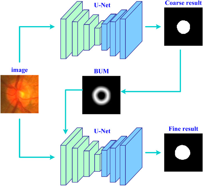
Figure 1. The flowchart of the developed deep learning strategy based on the U-Net for accurate image segmentation.
2.2 Object coarse segmentation
We first trained the U-Net based on the given images and their manual annotations leveraging a plain network training scheme to obtain a relatively coarse segmentation result for desirable objects. This train procedure can be given by:
where
2.3 Boundary uncertainty map
The obtained coarse segmentation results were often different from manual annotations of objects in certain image regions, especially object boundary regions, but they can provide some important position information for desirable objects. To effectively use the position information, we processed the coarse segmentation results leveraging morphological dilation and erosion operations (Fang et al., 2021), leading to two different object regions. Based on the two object regions, we can identify a potential boundary region (PBR) and a background excluded image (BEI) for each target object, which were separately given by
where
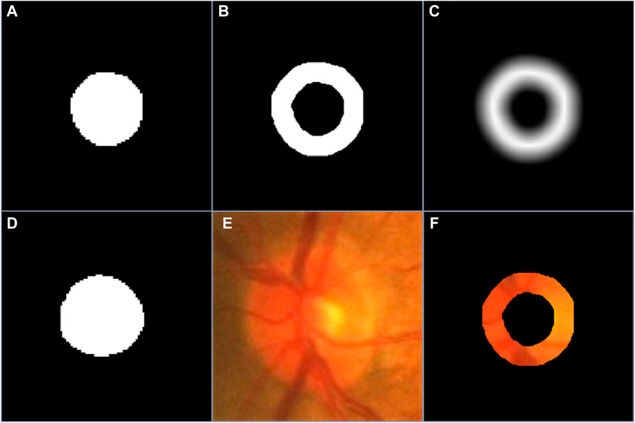
Figure 2. (A–C) are the coarse segmentation result, the PBR and boundary uncertainty map, respectively, (D–F) are the manual annotation of desirable object, the original image and its background excluded version.
2.4 Object fine segmentation
After obtaining the boundary uncertainty map and background excluded image, we concatenated these two types of images and fed them into the segmentation network. Since the concatenated images were different from the original images and contained very little background information, the segmentation network can easily detect object boundaries and thereby extract the whole object regions accurately using a simple experiment configuration. Specifically, we implemented the fine segmentation of desirable objects using the same configuration as their coarse segmentation (e.g., the cost function, optimizer and batch size).
2.5 Experiment datasets
To validate the developed learning strategy, we performed a series of segmentation experiments on two public dataset, as shown in Figure 3. The first dataset was from the Retinal Fundus Glaucoma Challenge (REFUGE) (Orlando et al., 2020) and contained 1,200 retinal fundus images acquired by two different cameras, together with manual annotations for the optic disc (OD) and cup (OC) regions. These images and their annotations were evenly split into three subsets for training (n = 400), validation (n = 400) and testing (n = 400) purposes, respectively, in the REFUGE challenge, which were also used in this study for segmentation purposes. We normalized these images to reduce the influence of light exposure and cameras and then extracted local disc patches using the dimensions that approximated three times the radius of the OD regions (Wang et al., 2021b). The extracted patches were then resized to 256 × 256 pixels and fed into the U-Net for network training.
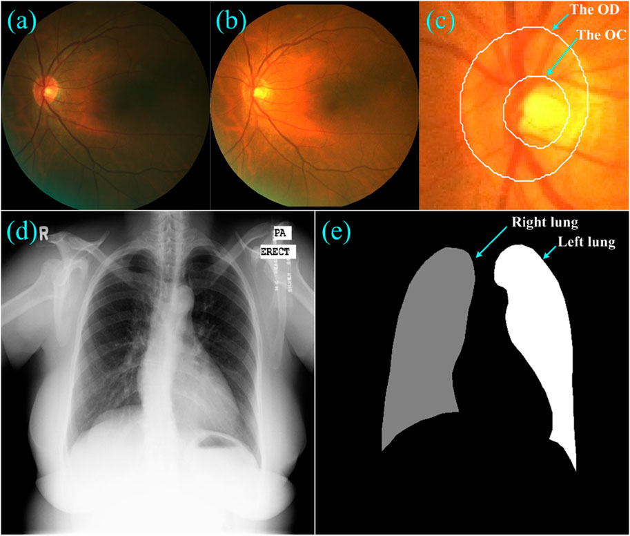
Figure 3. (A–C) showed a fundus image, its normalized version, and the local disc patch with manual annotations of the OD and OC, respectively, (D) and (E) showed a Xray image and its annotations for the left and right lungs.
The second dataset was from a tuberculosis screening program in Montgomery County (TSMC) (Jaeger et al., 2014) and contained 138 chest Xray images acquired using a Eureka stationary Xray machine. Among these Xray images, 80 were normal and 58 were abnormal with manifestations of tuberculosis. All images were de-identified and had a dimension of either 4,020 × 4,892 or 4,892 × 4,020 pixels. The left and right lungs depicted on these Xray images were manually annotated by a radiologist. We also split these Xray images equally into three disjoint subsets for network training (n = 46), validation (n = 46) and testing (n = 46), and resized them to the same dimension of 256 × 256 pixels.
2.6 Performance evaluation
We assessed the performance of the UGLS based on the U-Net (short for the developed method, https://github.com/wmuLei/ODsegmentation) on a 64-bit Windows 10 PC with 2.20 GHz 2.19 GHz Intel(R) Xeon(R) Gold 5120 CPU, 64 GB RAM and NVIDIA GeForce GTX 2080Ti by segmenting 1) the OC region from color fundus images and 2) the left and right lungs from the Xray images, where the
where
With these output results, we evaluated our developed method using the DS, Matthew’s correlation coefficient (MCC) (Zhu, 2020), sensitivity (SEN) (Wang et al., 2019), and Hausdorff distance (HSD, in pixel).
where
3 Results
3.1 Object coarse segmentation
Tables 1 and 2 summarized six coarse segmentation results of the U-Net with the developed UGLS strategy in extracting the OC from retinal fundus images and the left and right lungs from Xray images, respectively. As demonstrated by the results, the U-Net achieved a relatively low performance in segmenting the OC depicted on fundus images (due to the high similarity between the OD and OC regions), with a average DS, MCC, SEN and HSD of 0.8642, 0.8585, 0.8674 and 2.6420, respectively. In contrast, it obtained a better accuracy for the left and right lungs (with the average DS of 0.9408 and 0.9477, respectively) and can compete with their manual annotations.
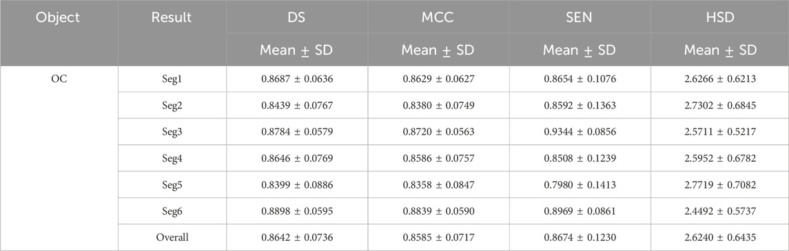
Table 1. Results of our proposed method for the coarse segmentation of the OC regions based on six experiments (i.e., Seg1-6) in terms of the mean and standard deviation (SD) of DS, MCC, SEN and HSD (in pixel).
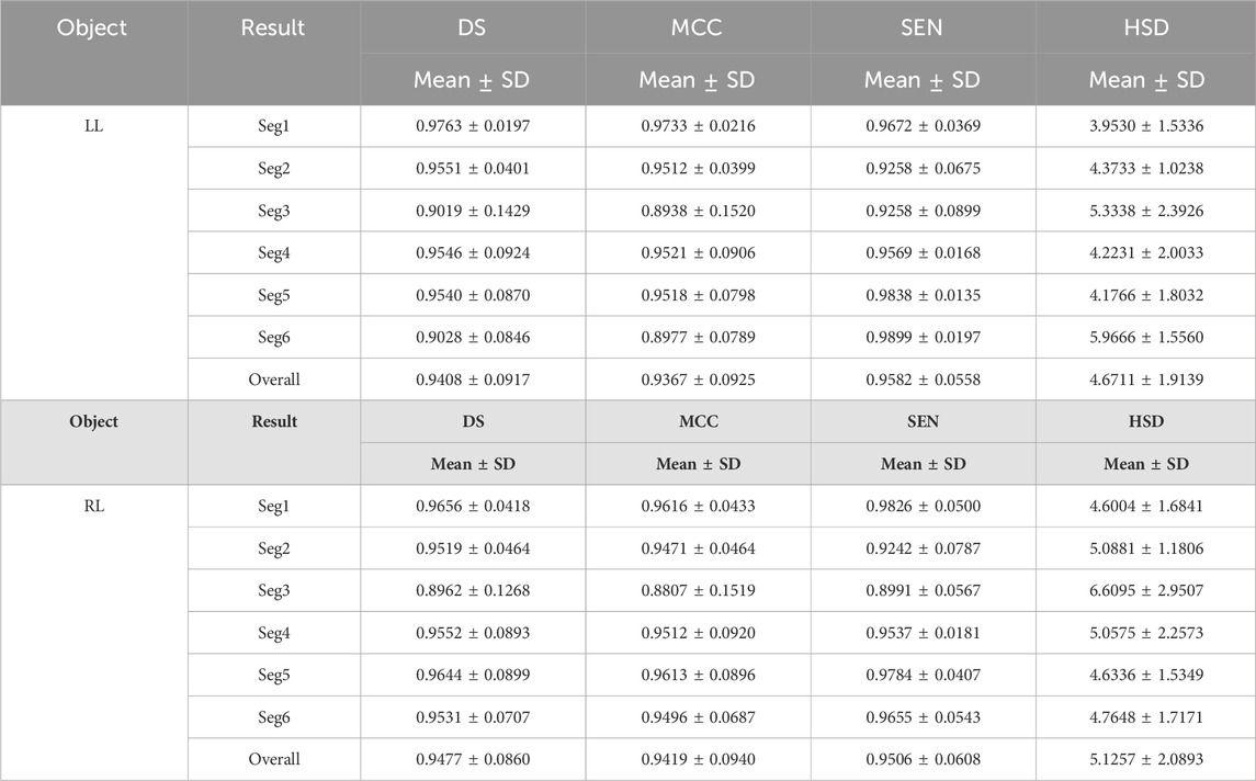
Table 2. The performance of the developed method for segmenting the left and right lungs (LL and RL) from Xray images.
3.2 Object fine segmentation
Tables 3 and 4 demonstrated the fine segmentation results of the U-Net with the developed UGLS strategy for three different objects depicted on fundus and Xray images, respectively. The U-Net achieved the average DS and SEN of 0.8791 and 0.8858 for the OC region, and 0.9605, 0.9607, 0.9621, and 0.9668 for the left and righ lungs, respectively. As compared with its coarse segmentation results, the U-Net obtained a significantly better overall performance for six different experiments on two types of images with varying modalities (p < 0.01). Specifically, the U-Net had better performances for five fine segmentation experiments for the OC, as compared to its coarse results, as shown in Table 3. Similarly, its performances were also increased in large increments for each experiment in the fine segmentation of the left and right lungs.
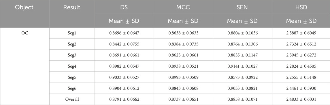
Table 3. Fine segmentation results of the developed method for the OC regions in terms of the DS, MCC, SEN and HSD (in pixel) metrics.
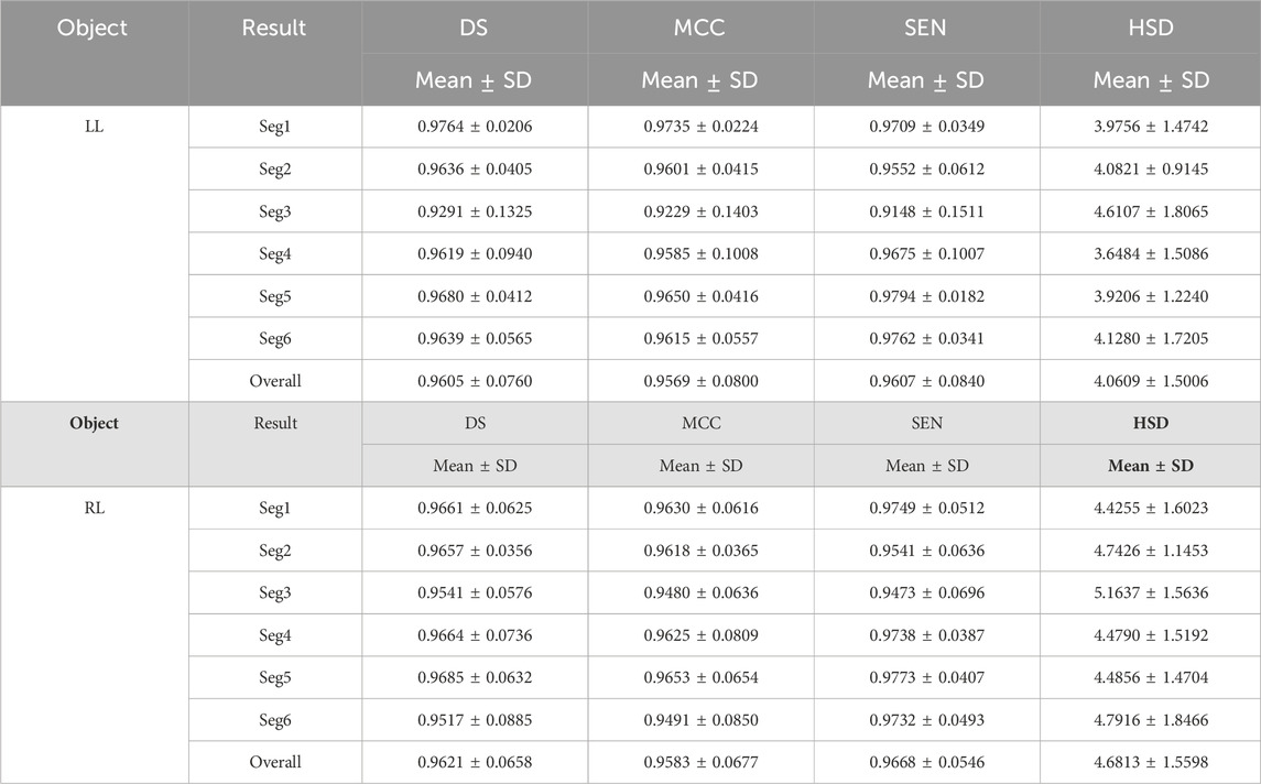
Table 4. Fine segmentation results of the developed method for segmenting the left and right lungs (LL and RL) from the Xray images in terms of the DS, MCC, SEN and HSD (in pixel) metrics.
3.3 Performance comparison
Table 5 summarized the segmentation results of the involved networks (i.e., the U-Net, AU-Net, BiO-Net, AS-Net, Swin-Unet, and TransUNet) in extracting three different objects from fund and Xray images, respectively. As demonstrated by these results, the developed UGLS strategy can significantly improve the performance of the U-Net (p < 0.01) by merely leveraging the its coarse segmentation results in a reasonable way, instead of changing its network structure. Specifically, the average DS of the U-Net increased from 0.8792 to 0.8945 for three different object regions depicted on fundus and Xray images after using our developed deep learning strategy. This strategy made our developed method superior or comparable to the AU-Net (0.8803, p < 0.001), BiO-Net (0.8843, p < 0.005), AS-Net (0.8859, p < 0.005), Swin-Unet (0.8811, p < 0.001), and TransUNet (0.8900, p < 0.05) with all the p-values less than 0.05 for the two segmentation tasks. Figures 4 and 5 showed the performance differences among the involved networks on several fundus and Xray images.
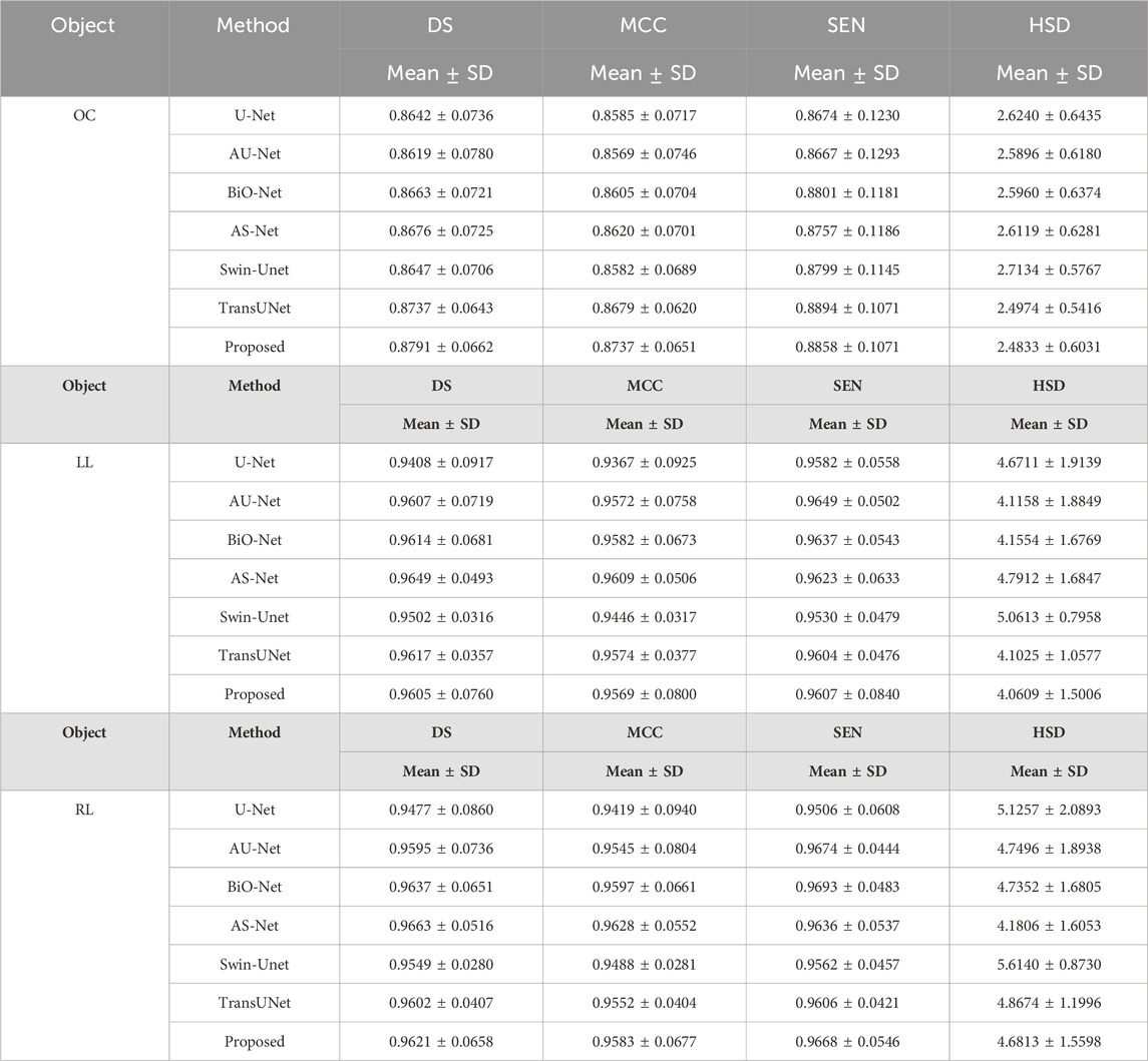
Table 5. Performance differences among the involved networks in segmenting the OC, left and right lungs depicted on fundus and Xray images, respectively.
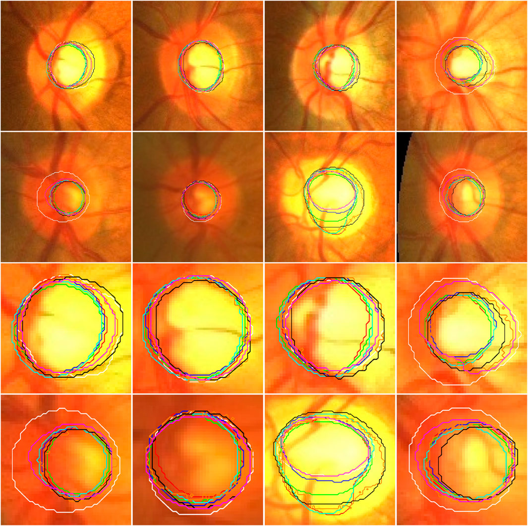
Figure 4. Illustration of the segmentation results of local disc patches (in the first two rows) and their closeup versions (in the last two rows) from eight fundus images obtained by the AU-Net (in green), BiO-Net (in blue), AS-Net (in cyan), Swin-Unet (in black), TransUNet (in orange) and our developed method in coarse (in red) and fine (in magenta) segmentation stages as well as their manual delineations (in white), respectively.
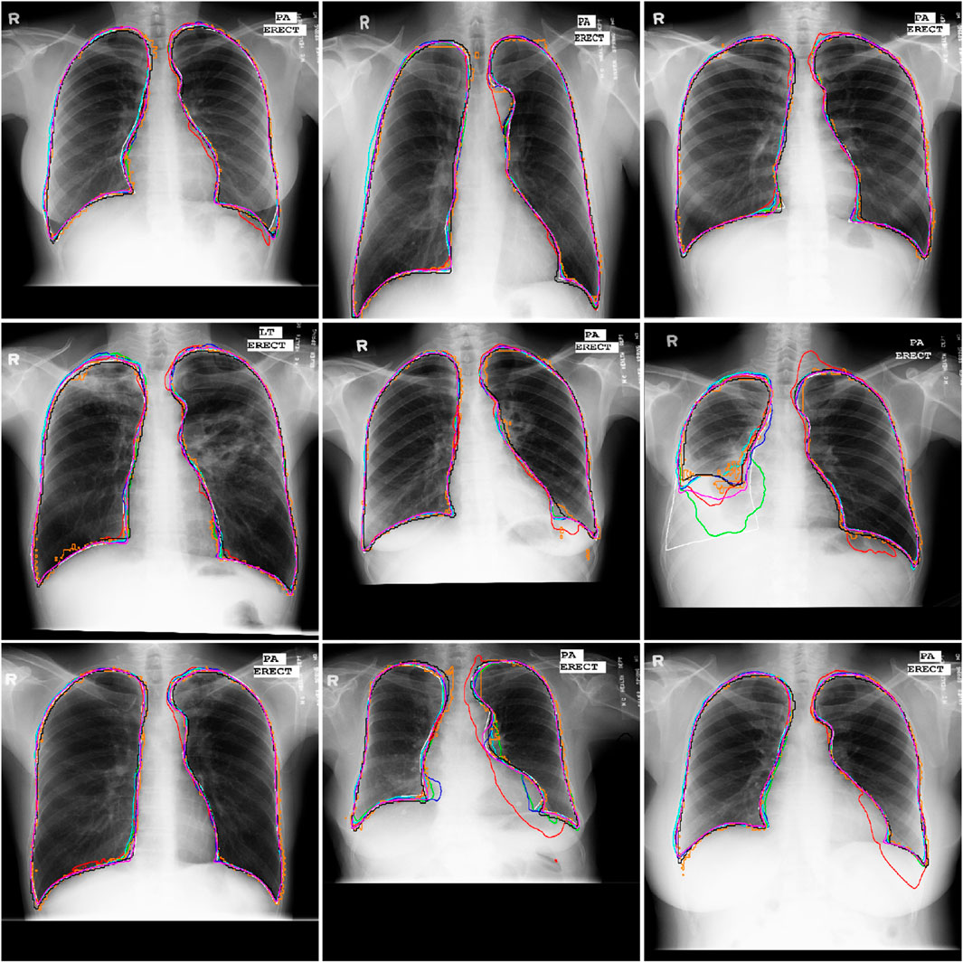
Figure 5. Illustration of the segmentation results of nine Xray images obtained by the AU-Net (in green), BiO-Net (in blue), AS-Net (in cyan), Swin-Unet (in black), TransUNet (in orange) and our developed method in coarse (in red) and fine (in magenta) segmentation stages as well as their manual delineations (in white), respectively.
3.4 Effect of the BUM
Table 6 showed the results of the developed method in extracting the left and right lungs from Xray images using boundary uncertainty maps in three different ways. As demonstrated by the results, our developed method obtained the lowest segmentation performance, with the average DS of 0.9437 when merely trained on boundary uncertainty maps, but it had increased performance when combining the uncertainty maps with the original images or their background excluded version for network training (with the average DS of 0.9611 and 0.9613). Moreover, the background excluded images can better improve the performance of our developed method since they reduced the impact of irrelevant background information away from desirable objects.

Table 6. The results of the developed method trained on the boundary uncertainty map (BUM) or its combination with the original image (ORI) or its background excluded version (BEI) for the left and right lung segmentation.
3.5 Effect of parameter
Table 7 summarized the impact of the parameter
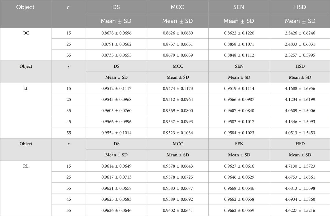
Table 7. The results of the developed method on fundus and Xray images by setting different values for parameters
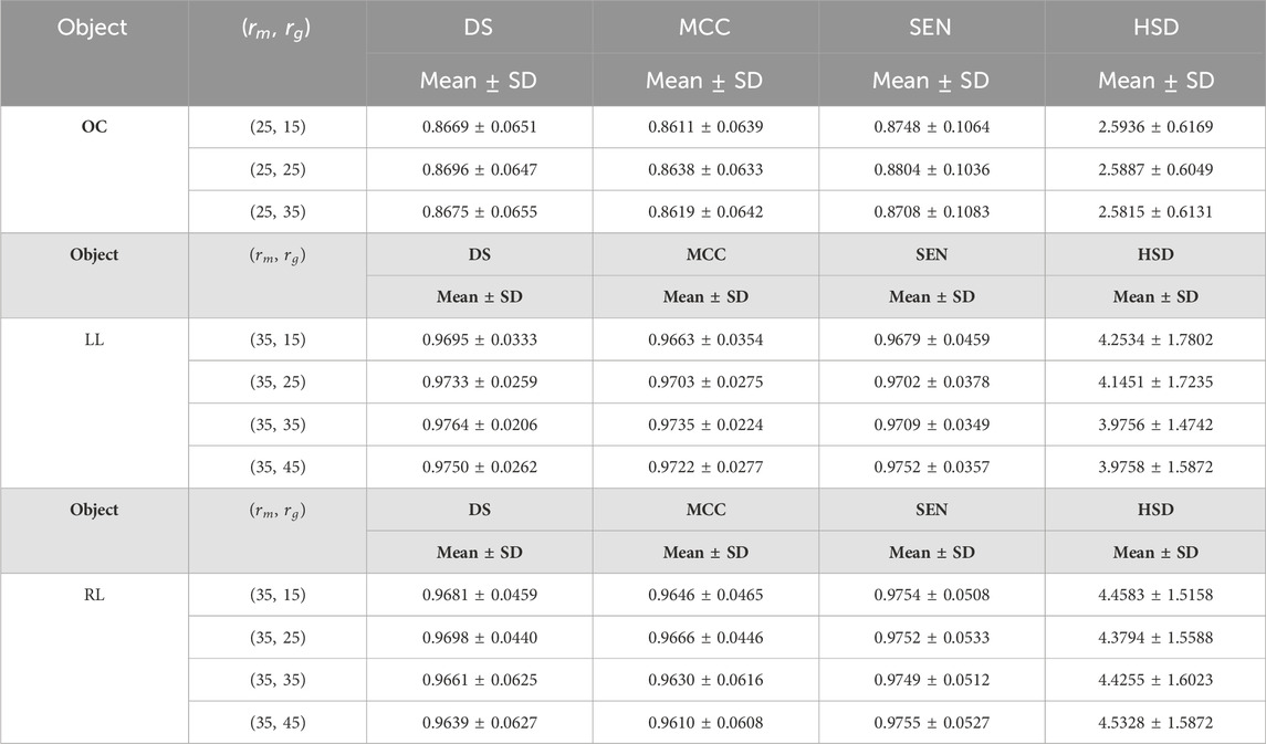
Table 8. The results of the developed method for the first experiment on fundus and Xray images using different values for parameter
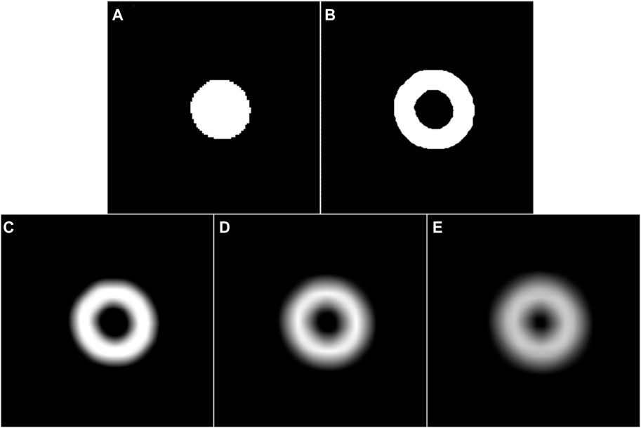
Figure 6. (A) and (B) are the coarse segmentation result of a given fundus image and its corresponding potential boundary region, respectively. (C–E) are the smoothed results of (B) using a Gassian filter with the parameter
4 Discussion
In this paper, we developed a novel network training strategy (termed UGLS) for accurate image segmentation and assessed its effectiveness based on an existing network (i.e., the U-Net) by extracting three different objects depicted (i.e., the OC, left and right lungs) on fundus and Xray images. In the developed method, the U-Net was first trained using the traditional training strategy on the original images and their manual annotations for the coarse-grained segmentation of desirable objects. The segmentation results were then proposed to locate a potential boundary region for each object, which was combined with the original images for the fine segmentation of the objects. We validated the developed method on two public datasets (i.e., REFUGE and TSMC) and compared it with five available networks (i.e., the AU-Net, BiO-Net, AS-Net, Swin-Unet and TransUNet) under the similar experiment configurations. Extensive experiments showed that the developed method can largely improve the segmentation performance of the U-Net and was comparable or superior to the AU-Net, BiO-Net, AS-Net, Swin-Unet and TransUNet, all of which had much more complex network structures than the U-Net.
The developed method achieved promising overall performance in segmenting multiple different objects, as compared to three existing networks. This may be attributed to the following reasons: First, the coarse segmentation of the objects was able to detect various types of image features and provide some important location information for each object and its boundaries. Second, the introduction of boundary uncertainty maps made the potential boundary region have a unique intensity distribution. This distribution largely facilitated the detection of object boundaries and enhanced the sensitivity and accuracy of the U-Net in segmenting objects of interest. Third, the use of background excluded images can not only ensure a reasonable balance between object information and its surrounding background, but also ensure that the U-Net performs the learning of various features in the specified region, thereby leading to a increased segmentation performance and a reduced influence of undesirable background. Due to these reasons, the developed method can significantly improve the segmentation performance of a relatively simple network (i.e., the U-Net) and make it comparable or superior to several existing sophisticated networks.
We further assessed the influence of boundary uncertainty maps and the parameter
5 Conclusion
We developed a uncertainty guided deep learning strategy (UGLS) to improve the performance of existing segmentation neural networks and validated it based on the classical U-Net by segmenting the OC from color fundus images and the left and right lungs from Xray images. The novelty of our developed method lies in the introduction of boundary uncertainty maps and their integration with the input images for accurate image segmentation. Extensive experiments on public fundus and Xray image datasets demonstrated that the developed method had the potential to effectively extract the OC from fundus images and the left and right lungs from Xray images, largely improved the performance of the U-Net, and can compete with several sophisticated networks (i.e., the AU-Net, BiO-Net, AS-Net, Swin-Net, and TransUNet).
Data availability statement
Publicly available datasets were analyzed in this study. This data can be found here: Retinal Fundus Glaucoma Challenge (REFUGE), a tuberculosis screening program in Montgomery County.
Author contributions
XY: Methodology, Software, Writing–original draft. YZ: Resources, Validation, Writing–original draft. CM: Formal Analysis, Investigation, Visualization, Writing–review and editing. GJ: Methodology, Software, Visualization, Writing–original draft. BT: Investigation, Validation, Visualization, Writing–original draft. LW: Methodology, Supervision, Writing–review and editing.
Funding
The author(s) declare that financial support was received for the research, authorship, and/or publication of this article. This work is supported in part by Natural Science Foundation of Zhejiang Province (Grant No. LGF22H090022 and LTGY23H090014), Health Commission of Zhejiang Province (Grant No. 2022KY1206), and Wenzhou Municipal Science and Technology Bureau (Grant No. ZY2022024).
Conflict of interest
The authors declare that the research was conducted in the absence of any commercial or financial relationships that could be construed as a potential conflict of interest.
Publisher’s note
All claims expressed in this article are solely those of the authors and do not necessarily represent those of their affiliated organizations, or those of the publisher, the editors and the reviewers. Any product that may be evaluated in this article, or claim that may be made by its manufacturer, is not guaranteed or endorsed by the publisher.
References
Alom M. Z., Yakopcic C., Hasan M., Taha T. M., Asari V. K. (2019). Recurrent residual U-Net for medical image segmentation. J. Med. Imaging (Bellingham) 6, 014006. doi:10.1117/1.Jmi.6.1.014006
Cao H., Wang Y., Chen J., Jiang D., Zhang X., Tian Q., et al. (2022). Swin-unet: unet-like pure transformer for medical image segmentation. Eur. Conf. Comput. Vis. (ECCV).
Chen J., Lu Y., Yu Q., Luo X., Adeli E., Wang Y., et al. “TransUNet: transformers make strong encoders for medical image segmentation,” in 2021 IEEE/CVF Conference on Computer Vision and Pattern, Nashville, TN, USA, June 2021.
Fang X., Shen Y., Zheng B., Zhu S., Wu M. “Optic disc segmentation based on phase-fusion PSPNet,” in Proceedings of the 2nd International Symposium on Artificial Intelligence for Medicine Sciences, Beijing, China, October 2021 (Association for Computing Machinery).
Gawlikowski J., Tassi C., Ali M., Lee J., Humt M., Feng J., et al. (2023). A survey of uncertainty in deep neural networks. Artif. Intell. Rev. 56, 1513–1589. doi:10.1007/s10462-023-10562-9
Han D. J. J. O. I., Graphics (2006). A survey on image segmentation using active contour and level set method. Neurocomputing 452. doi:10.1016/j.neucom.2020.07.141
Hossain N. I., Reza S. “Blood vessel detection from fundus image using Markov random field based image segmentation,” in 2017 4th International Conference on Advances in Electrical Engineering ICAEE, Dhaka, Bangladesh, 28-30 September 2017, 123–127.
Huang H., Lin L., Tong R., Hu H., Zhang Q., Iwamoto Y., et al. “UNet 3+: a full-scale connected UNet for medical image segmentation,” in ICASSP 2020 - 2020 IEEE International Conference on Acoustics, Speech and Signal Processing ICASSP, Barcelona, Spain, 4-8 May 2020, 1055–1059.
Jaeger S., Candemir S., Antani S., Wáng Y. X., Lu P. X., Thoma G. (2014). Two public chest X-ray datasets for computer-aided screening of pulmonary diseases. Quant. Imaging Med. Surg. 4, 475–477. doi:10.3978/j.issn.2223-4292.2014.11.20
Jun T. J., Kweon J., Kim Y. H., Kim D. (2020). T-Net: nested encoder-decoder architecture for the main vessel segmentation in coronary angiography. Neural Netw. 128, 216–233. doi:10.1016/j.neunet.2020.05.002
Khened M., Varghese A., Krishnamurthi G. J. M. I. A. (2018). Fully convolutional multi-scale residual DenseNets for cardiac segmentation and automated cardiac diagnosis using ensemble of classifiers. Med. Image Anal. 51, 21–45. doi:10.1016/j.media.2018.10.004
Li W., Li J., Polson J., Wang Z., Speier W., Arnold C. (2022). High resolution histopathology image generation and segmentation through adversarial training. Med. Image Anal. 75, 102251. doi:10.1016/j.media.2021.102251
Oktay O., Schlemper J., Folgoc L. L., Lee M. J., Heinrich M. P., Misawa K., et al. (2018). Attention U-net: learning where to look for the pancreas. https://arxiv.org/abs/1804.03999.
Orlando J. I., Fu H., Barbosa Breda J., Van Keer K., Bathula D. R., Diaz-Pinto A., et al. (2020). REFUGE Challenge: a unified framework for evaluating automated methods for glaucoma assessment from fundus photographs. Med. Image Anal. 59, 101570. doi:10.1016/j.media.2019.101570
Pare S., Kumar A., Singh G. K., Bajaj V. J. I. J. O. S., Technology T. O. E. E. (2019). Image segmentation using multilevel thresholding: a research review. Iran. J. Sci. Technol. Trans. Electr. Eng. 44, 1–29. doi:10.1007/s40998-019-00251-1
Poggi G., Ragozini R. P. (1999). Image segmentation by tree-structured Markov random fields. IEEE Signal Process. Lett. 6, 155–157. doi:10.1109/97.769356
Ronneberger O., Fischer P., Brox T. (2015). “U-net: convolutional networks for biomedical image segmentation,” in Medical image computing and computer-assisted intervention – miccai 2015. Editors N. Navab, J. Hornegger, W. M. Wells, and A. F. Frangi (Cham: Springer International Publishing), 234–241.
Seo H., Huang C., Bassenne M., Xiao R., Xing L. (2020). Modified U-net (mU-Net) with incorporation of object-dependent high level features for improved liver and liver-tumor segmentation in CT images. IEEE Trans. Med. Imaging 39, 1316–1325. doi:10.1109/TMI.2019.2948320
Seoni S., Jahmunah V., Salvi M., Barua P., Molinari F., Acharya U. (2023). Application of uncertainty quantification to artificial intelligence in healthcare: a review of last decade (2013-2023). Comput. Biol. Med. 165, 107441. doi:10.1016/j.compbiomed.2023.107441
Shahamat H., Saniee Abadeh M. (2020). Brain MRI analysis using a deep learning based evolutionary approach. Neural Netw. 126, 218–234. doi:10.1016/j.neunet.2020.03.017
Shi C., Zhang J., Zhang X., Shen M., Chen H., Wang L. (2022). A recurrent skip deep learning network for accurate image segmentation. Biomed. Signal Process. Control 74, 103533. doi:10.1016/j.bspc.2022.103533
Wang L., Chen K., Wen H., Zheng Q., Chen Y., Pu J., et al. (2021a). Feasibility assessment of infectious keratitis depicted on slit-lamp and smartphone photographs using deep learning. Int. J. Med. Inf. 155, 104583. doi:10.1016/j.ijmedinf.2021.104583
Wang L., Gu J., Chen Y., Liang Y., Zhang W., Pu J., et al. (2021b). Automated segmentation of the optic disc from fundus images using an asymmetric deep learning network. Pattern Recognit. 112, 107810. doi:10.1016/j.patcog.2020.107810
Wang L., Liu H., Lu Y., Chen H., Zhang J., Pu J. (2019). A coarse-to-fine deep learning framework for optic disc segmentation in fundus images. Biomed. Signal Process. Control 51, 82–89. doi:10.1016/j.bspc.2019.01.022
Wang L., Shen M., Chang Q., Shi C., Chen Y., Zhou Y., et al. (2021c). Automated delineation of corneal layers on OCT images using a boundary-guided CNN. Pattern Recognit. 120, 108158. doi:10.1016/j.patcog.2021.108158
Wang L., Shen M., Shi C., Zhou Y., Chen Y., Pu J., et al. (2022). EE-Net: an edge-enhanced deep learning network for jointly identifying corneal micro-layers from optical coherence tomography. Biomed. Signal Process. Control 71, 103213. doi:10.1016/j.bspc.2021.103213
Wang Y., Yu X., Wu C. (2022). An efficient hierarchical optic disc and cup segmentation network combined with multi-task learning and adversarial learning. J. Digit. Imaging 35, 638–653. doi:10.1007/s10278-021-00579-3
Xiang T., Zhang C., Liu D., Song Y., Huang H., Cai W. (2020). “BiO-net: learning recurrent Bi-directional connections for encoder-decoder architecture,” in Medical image computing and computer assisted intervention – miccai 2020. Editors A. L. Martel, P. Abolmaesumi, D. Stoyanov, D. Mateus, M. A. Zuluaga, S. K. Zhouet al. (Cham: Springer International Publishing), 74–84.
Zhang J., Mei C., Li Z., Ying J., Zheng Q., Yi Q., et al. (2023). Automated segmentation of optic disc and cup depicted on color fundus images using a distance-guided deep learning strategy. Biomed. Signal Process. Control 86, 105163. doi:10.1016/j.bspc.2023.105163
Zheng Q., Zhang X., Zhang J., Bai F., Huang S., Pu J., et al. (2022). A texture-aware U-Net for identifying incomplete blinking from eye videography. Biomed. Signal Process. Control 75, 103630. doi:10.1016/j.bspc.2022.103630
Zhou Z., Rahman Siddiquee M. M., Tajbakhsh N., Liang J. (2018). “UNet++: a nested U-net architecture for medical image segmentation,” in Deep learning in medical image analysis and multimodal learning for clinical decision support. Editors D. Stoyanov, Z. Taylor, G. Carneiro, T. Syeda-Mahmood, A. Martel, L. Maier-Heinet al. (Cham: Springer International Publishing), 3–11.
Keywords: deep learning, training strategy, image segmentation, fundus image, optic cup deep learning, optic cup
Citation: Yang X, Zheng Y, Mei C, Jiang G, Tian B and Wang L (2024) UGLS: an uncertainty guided deep learning strategy for accurate image segmentation. Front. Physiol. 15:1362386. doi: 10.3389/fphys.2024.1362386
Received: 05 January 2024; Accepted: 26 March 2024;
Published: 08 April 2024.
Edited by:
Cristiana Corsi, University of Bologna, ItalyReviewed by:
Massimo Salvi, Polytechnic University of Turin, ItalyJolita Bernatavičienė, Vilnius University, Lithuania
Copyright © 2024 Yang, Zheng, Mei, Jiang, Tian and Wang. This is an open-access article distributed under the terms of the Creative Commons Attribution License (CC BY). The use, distribution or reproduction in other forums is permitted, provided the original author(s) and the copyright owner(s) are credited and that the original publication in this journal is cited, in accordance with accepted academic practice. No use, distribution or reproduction is permitted which does not comply with these terms.
*Correspondence: Lei Wang, bGVpLndhbmdAZXllLmFjLmNu
†These authors have contributed equally to this work and share first authorship