 Gianluca Gennarelli1
 Vittorio Emanuele Colonna2Carlo Noviello1Stefano Perna1,2
 Francesco Soldovieri1
 Ilaria Catapano1*
- 1Institute for Electromagnetic Sensing of the Environment, National Research Council of Italy, Napoli, Italy
- 2Department of Engineering (DI), Università Degli Studi di Napoli “Parthenope”, Napoli, Italy
Indoor occupancy sensing is a crucial problem in several application fields that have progressed from intrusion detection systems to automatic control of lighting, heating, air conditioning and many other presence-related loads. Continuous wave Doppler radar is a simple technology to face this problem due to its capability to detect human body movements (e.g., walk, run) and small chest wall vibrations associated to the cardiorespiratory activity. This work deals with a radar prototype operating at 2.4 GHz as a real-time occupancy sensor. The emphasis is on data processing approaches devoted to extract useful information from raw radar signal. Three different strategies, designed to detect human presence in indoor environments, are considered and the main goal is the assessment and comparison of their performance against experimental data collected in controlled conditions. The first strategy is based on the analysis of the standard deviation of the radar signal in time-domain; whereas the second one exploits the histogram of the time-varying signal amplitude. Finally, a third strategy based on an energy measure of the received signal Doppler spectrum is considered. The proposed detection algorithms are optimized through a set of calibration measurements and their performances and robustness are assessed by laboratory trials.
1 Introduction
Occupancy sensors, originally developed for intrusion detection systems, attract considerable interest in home automation and energy saving applications (Ahmad et al., 2021). Indeed, they are regularly used for the control of lighting, heating, ventilation, air conditioning (HVAC), and many other presence-related loads allowing a reduction up to 80% of the energy in residential, commercial and public spaces (EPRI, 1994).
The most common occupancy sensors are passive infrared (PIR) and ultrasonic sensors (Yavari et al., 2014). PIR sensors are motion detectors that detect large body movements such as walking and running; however, they are not sensitive to small movements (e.g., writing). PIR sensors operate only in line of sight and suffer from a high false alarm rate (Yatman et al., 2015). Ultrasonic sensors emit an acoustic wave in the 25–40 KHz band, imperceptible to the human ear, and detect the frequency shift of the backscattered signal caused by the Doppler effect when a target moves within the monitored area. Ultrasonic sensors are not entirely limited to the line of sight; within certain limits, through reflection and diffraction phenomena, it is possible to overcome a fixed obstacle and detect a moving person (Yavari et al., 2014). However, it is not possible to detect a person behind a wall due to the jump of acoustic impedance at the air-wall interface, which causes only a minimal signal penetration. Ultrasonic sensors are more expensive than PIR ones and can interfere with other hearing aids. Moreover, they are sensitive to air flows and, thus, they can generate false alarms (Yavari et al., 2014). Hybrid sensors based on both infrared and ultrasonic technologies have been developed to reduce the number of false alarms. These sensors are more expensive than PIR and ultrasonic sensors alone and are suitable for large open spaces (Steiner, 2009).
In recent years, Continuous Wave (CW) Doppler radar (Li and Lin, 2014; Li et al., 2013) has emerged as a simple and cost-effective technological solution for human detection in indoor environments. This type of radar exploits the phase modulation of the signal (Doppler effect) caused by human movements and small physiological displacements of the human chest wall related to the cardiopulmonary activity.
CW radar sensors were first introduced in the 1970s showing the possibility to detect vital parameters remotely (Lin, 1975; Lin, 1979). Since then, significant technological advances have been made both on hardware (e.g., sensor miniaturization, sensitivity improvement, etc.) and signal processing algorithms (Li and Lin, 2014; Li et al., 2013; Tang et al., 2014). The exploitation of CW Doppler radars has been suggested in several application contexts. In healthcare, for instance, they are often referred to as “bioradars” and can be employed to detect sleep apneas (Alekhin et al., 2013; Baboli et al., 2015) or mental stress (Fernàndez and Anishchenko, 2018) in humans, and breathing disorders in living animals (Anishchenko et al., 2015). Moreover, the application of CW bioradars has been suggested also for preventing the sudden infant death syndrome (Li et al., 2009), tumor tracking in radiation therapy (Li and Lin, 2014), and cardiac motion imaging (Wang et al., 2013). The main advantage offered by a bioradar is the possibility to avoid contact electrodes or probes. These last may be uncomfortable for the patient, especially when a long monitoring is required as during tests to diagnose sleep disorders (e.g., polysomnography). In addition, there are also situations where it is difficult to apply contact sensors, as in the case of patients suffering from severe burns. A metrological characterization of a bioradar as a tool to measure the breathing rate of a human has been reported in (Cerasuolo et al., 2017). In ambient assisted living and elderly care, CW radars have been proposed to recognize human gait and detect falls (Geisheimer et al., 2001; Otero, 2005; Hornsteiner and Detlefsen, 2008; Dremina and Anishchenko, 2016) while, in security applications, they can be used to get situation awareness in through the wall scenarios (Lubecke et al., 2007; Gennarelli et al., 2016). CW radar prototypes with frequency modulation have been recently developed also for airborne synthetic aperture radar applications, e.g., see (Aguasca et al., 2013; Meta et al., 2007; Esposito et al., 2020).
This paper deals with a CW Doppler radar prototype ad-hoc designed to be used as presence detector for real-time surveillance of indoor environments. The sensor is a compact portable device operating at the frequency of 2.45 GHz. The main focus is on data processing algorithms to be applied to raw signals in order to detect moving or stationary subjects in the scene. Specifically, three different detection strategies are considered with the aim to estimate their performances and determine if one method is more suitable than the other ones in terms of detection accuracy and computation effectiveness. On the other hand, the availability of several performing approaches makes possible, in principle, the development of integrated techniques combining the outputs of different algorithms to further enhance the overall system reliability.
The first considered detection strategy has been previously reported in (Gennarelli et al., 2016) and is based on the standard deviation of the radar signal in time domain. The second strategy exploits the histogram of the signal amplitude, while the third detection scheme is based on an energy measure of the signal Doppler spectrum. Each data processing approach involves a detection threshold, which is determined thanks to an ad-hoc developed calibration strategy. Experimental results concerning two indoor scenarios are presented to appraise the performance of the detection strategies.
The article is structured as follows. Section 2 summarizes the CW radar architecture and the designed prototype. The three detection strategies are presented in Section 3. Experimental results are reported in Section 4. Concluding remarks follow in Section 5.
2 CW Radar Architecture and Prototype
2.1 Radar Architecture and Signal Model
The radar architecture is depicted in Figure 1 and is based on a dual channel direct conversion (zero IF) receiver. A radio frequency (RF) source emits a CW signal
where
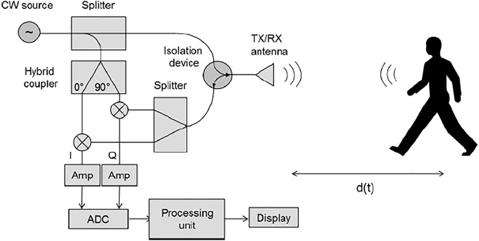
FIGURE 1. CW radar system architecture.
Let
where
The received signal at the output of the isolation device is split into two equal parts and demodulated by using the two reference signals with 90° phase offset. After, these two signals are amplified and filtered in order to reject the spectral components with frequency
where
According to Eqs 3, 4, the baseband signals
Note that different amplitude terms
2.2 Radar Prototype
A short range CW Doppler radar for occupancy sensing has been designed and developed (see Figure 2). The system has the architecture sketched in Figure 1 and generates a RF signal at 2.4 GHz thanks to a voltage-controlled oscillator. The chosen working frequency assures the possibility to operate within the Industrial, Scientific and Medical (ISM) band, i.e., the portion of the electromagnetic spectrum internationally reserved for industrial, scientific and medical use. Moreover, a 12.5 cm electromagnetic wavelength in free-space yields a good detection sensitivity for the detection of human targets.
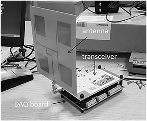
FIGURE 2. Radar prototype.
The prototype in Figure 2 comprises a RF front-end, a power supply section, and a baseband analog circuitry, which are all integrated on a double layer printed circuit board. The RF circuitry has been designed by using the microstrip technology. The antenna is a compact and low profile corporate fed 2 × 2 patch array with 10 dB gain and horizontal polarization.
The main technical parameters of the radar are summarized in Table 1. The radar emits a low power (<20 dBm) and has a short range coverage (about 20 m) and an angular coverage of ±50° both in elevation and azimuth with respect to the antenna boresight. Moreover, the electric field intensity 1 m far away from the antennas is lower than 1 V/m. Accordingly, the instrument complies with the Italian regulatory constraints on exposure to electromagnetic fields (D.P.C.M. 8/7/, 2003).

TABLE 1. Radar system parameters.
The baseband outputs are digitized by using a commercial data acquisition board (Measurement Computing mod. USB-2408) and sent to a laptop via USB. The laptop allows controlling the system as well as performing the real-time signal processing operations needed for the detection task. The software for data acquisition, processing and visualization has been implemented under MATLAB environment. In particular, a user friendly graphical user interface (GUI) has been developed to aid the management of the aforementioned operations (see Figure 3).
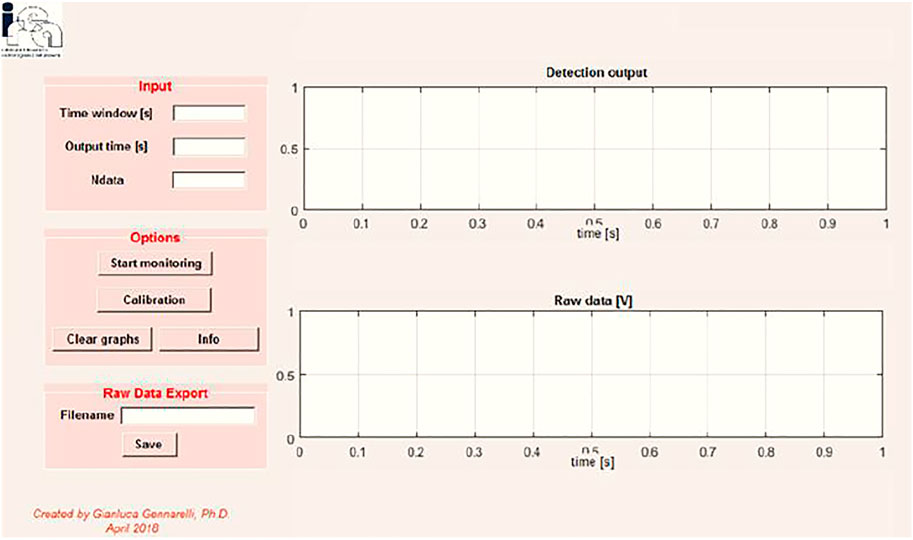
FIGURE 3. MATLAB GUI for data processing, acquisition and visualization.
3 Detection Strategies
This section summarizes the data processing strategies for real-time detection of human presence. The algorithms achieve automatic target detection based on different criteria and need a proper detection threshold. Such a threshold is determined thanks to a calibration procedure applied over reference datasets collected in known experimental conditions.
3.1 Standard Deviation Method
The presence of a target induces evident variations of the radar signal or equivalently increases the signal standard deviation (Gennarelli et al., 2016). The Standard Deviation Method (SDM) exploits this phenomenon to accomplish the occupancy sensing task.
Let us denote with yn, n = 1, … ,N, the discrete-time version of the radar signal y(t), N being the total number of samples in the observed sequence. Let
The detection strategy is based on the calculation of the standard deviation
where
Then, the following two hypotheses
where
The rule in Eq. 6 decides the hypothesis
The determination of the optimal threshold
where
It must be stressed that the window duration
3.2 Histogram Method
Experimental observations have shown that the amplitude of the radar signal is concentrated about the origin when no target is present in the scene, while it varies over a wider range when a target is present (Yavari et al., 2014; Gennarelli et al., 2016). A simple graphical representation to visualize this concept is provided by the histogram of amplitude levels. In particular, in the case of an empty scene, the histogram is concentrated around the origin, i.e. most signal samples fall in the central bin. On the contrary, when targets are stationary, the histogram becomes more spread and such spreading grows much more when they are moving.
The Histogram Method (HM) detects the presence of targets based on the percentage of signal samples with amplitude belonging to an interval (–
where
As for SDM, a calibration stage is essential to determine the optimal threshold
The choice of the time window T is a compromise between accuracy and system responsiveness as for the SDM.
3.3 Doppler Spectrum Energy Method
The Doppler spectrum of the radar signal provides an indication of the distribution of target’s speed and movements (Otero, 2005; Hornsteiner and Detlefsen, 2008). As the complexity of the scene increases (e.g., one or more targets in motion), the Doppler spectrum becomes more spread compared to a scenario with stationary targets.
The Doppler Spectrum Energy Method (DSEM) is based on the computation of the descriptor:
In the above formula,
The DSEM is based on the two hypotheses
where
According to Eq. 11, the hypothesis
Similarly to previous methods, the threshold
4 Experimental Tests
This section describes the results of experimental trials carried out in laboratory with the aim of evaluating the radar system capability to detect human presence and comparing the performance of the detection techniques introduced in Section 3. The tests were carried in two different indoor environments characterized by a different level of static clutter. The first one (Environment 1) is an empty landing with size 3 m × 8 m (see Figure 4). The second environment (Environment 2) is a laboratory containing different pieces of furniture (desk, tables, locker, etc.) and surrounded by plasterboard walls (see Figure 5). In all the tests, the radar was mounted at a height of 1.2 m above the ground and the signal was recorded over a time window of 60s with a sampling step of 0.08 s.
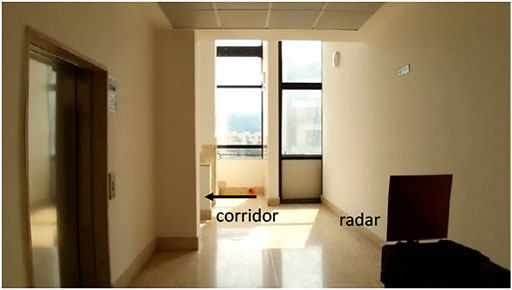
FIGURE 4. Photo of the landing (Environment 1).
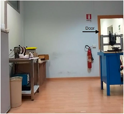
FIGURE 5. Photo of the laboratory (Environment 2).
4.1 Preliminary Tests
In the following, we show the results of some preliminary tests concerning the Environment 1 with the aim to check the system’s operation. During the first test, a person carried out various actions in the scene such as walk, stop, turn around, exit and enter the room. Figure 6 shows the radar signal in the time domain achieved after filtering the average value. When the person moves, the signal is characterized by strong fluctuations that become very intense as the subject approaches the radar. In the interval 18–24 s, the person stops and then the signal shows some periodic oscillations with lower amplitude that are related to the cardiorespiratory activity. At time t = 36 s, the subject leaves the scene taking the corridor indicated at the bottom left in Figure 4 and then re-enters the scene after 12 s. As can be seen in Figure 6, in the interval 36–48 s when the person is in the corridor, the radar signal is almost flat and its variability is essentially determined by system’s noise.
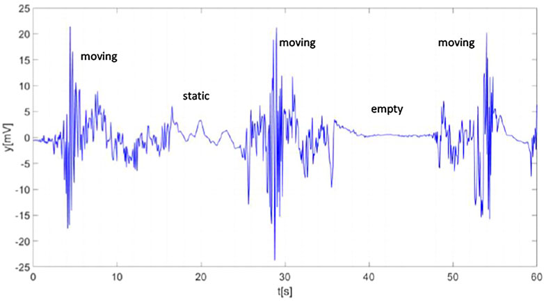
FIGURE 6. Radar signal after mean value filtering. Labels denote the actions performed by the subject.
The graphs in Figure 7 are useful to understand the HM operation. They show radar signals (top panels) and corresponding histograms of amplitude values (bottom panels) concerning three different scenarios. In detail, Figure 7A regards an empty scene and, in this case, a well-concentrated histogram around the origin is observed since about 90% of the signal samples fall in the central bin. In other words, the signal has an amplitude between –0.5 and 0.5 mV for 90% of the recording interval. On the other hand, when a stationary subject is present at 3 m distance (Figure 7B), the histogram is more spread and such spreading becomes even more evident when the subject is moving (Figure 7C).
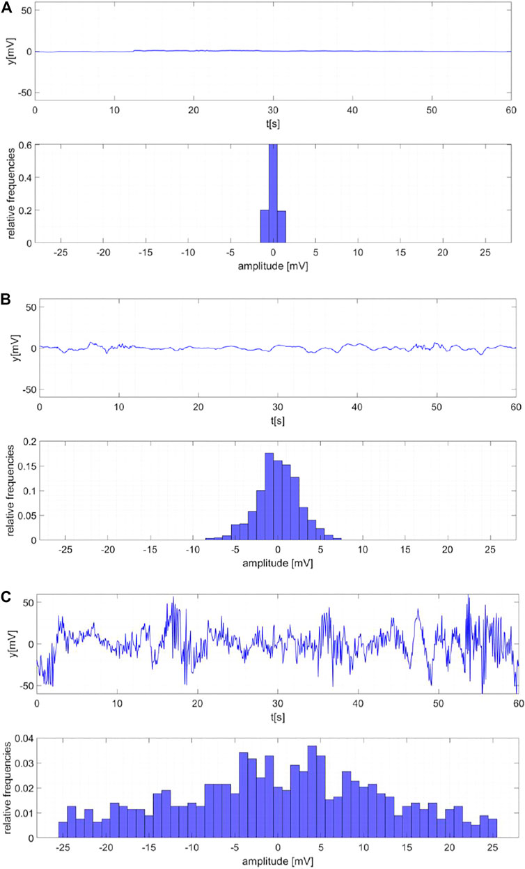
FIGURE 7. Radar signals (top panels) and corresponding histograms of amplitudes (bottom panels). Empty scene (A). Static subject 3 m far away from the radar (B). Moving subject (C).
The results illustrated in Figure 8 allow understanding the operation principle at the basis of DSEM. Specifically, they show radar signals (top panels) and corresponding spectrograms (bottom panels) concerning the scenarios described in Figure 7. The spectrograms are determined by plotting the short-time Fourier transforms of the signal over time windows having duration of 3 s and overlap of 2.9 s. As can be observed, the Doppler band is essentially null in the case of empty scene (Figure 8A). When a static target is present at 3 m distance (Figure 8B), it is possible to notice a slight increase in the amplitude of some spectral components around the typical frequencies of respiratory activity (0.2–0.4 Hz) (Cerasuolo et al., 2017). Finally, if the person walks around (Figure 8C), the spectrum has a significant amplitude at different frequencies.
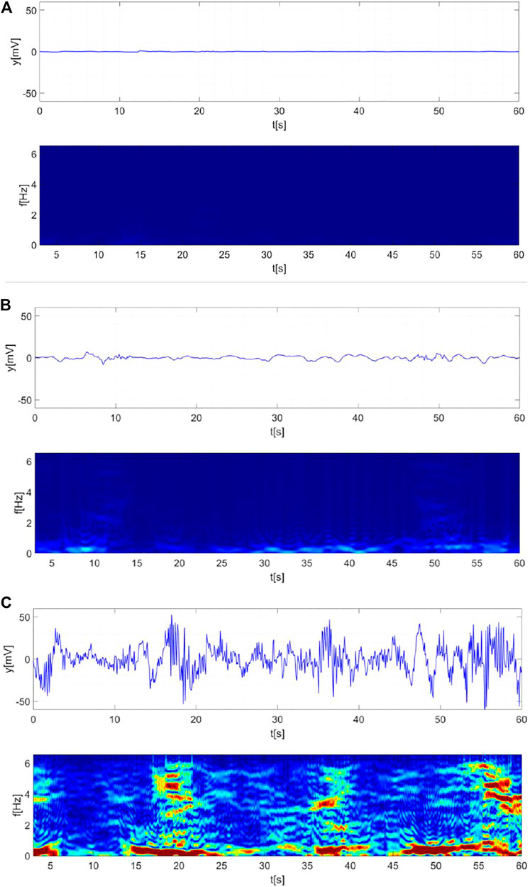
FIGURE 8. Radar signals (top panels) and normalized Doppler spectra (bottom panels). Empty scene (A). Static subject 3 m far away from the radar (B). Moving subject (C). Color scale [0, 0.4].
4.2 Sensor Calibration
In the following, we describe the results of the calibration procedure for each detection strategy. Six calibration datasets were recorded in Environment 1, each having a duration of 60 s. The first two acquisitions were made when the scene was empty, the third and fourth acquisitions were made when a person (an adult male) was stationary 2 and 3 m away from the radar, respectively. The last two recordings were made when a person was moving during the whole acquisition. The window duration T = 3 s has been found as the optimal compromise in terms of detection performance and system’s responsiveness.
The determination of the threshold
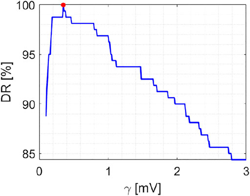
FIGURE 9. Calibration step. DR versus threshold
As regards HM calibration, this technique requires setting two parameters: half-width
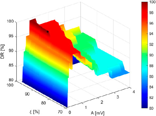
FIGURE 10. Calibration step. DR versus (
The calibration operation has been performed also for the DSEM based on Eq. 12 and Figure 11 reports the DR versus threshold. ψ As can be observed, the DR is maximal (about 100%) when ψ = ψ* = 0.84 · 10–3 mV2s (see asterisk in Figure 11).
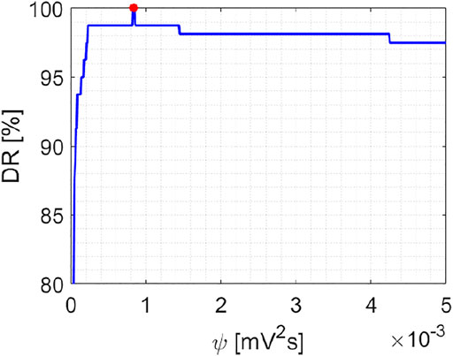
FIGURE 11. Calibration step. DR versus threshold ψ for DSEM. The optimal threshold
The calibration operation has been repeated for Environment 2 by processing six calibration datasets collected in experimental conditions similar to those recorded in Environment 1.
Table 2 summarizes the detection thresholds for each detection strategy and calibration environment. It can be observed that the SDM and DSEM thresholds attained in the Environment 2 are higher than those provided by calibration in the Environment 1. Moreover, the comparison between the HM thresholds shows that the percentage of samples are quite similar to each other while the half-width A is larger in the Environment 2. The higher thresholds of Environment 2 suggest that this environment is noisier probably due to the presence of several static scatterers (see Figure 5) and electromagnetic disturbances produced by Wi-Fi signals present in the building, which are not shielded by the plasterboard walls.

TABLE 2. Detection thresholds achieved for each environment and strategy.
4.3 Experimental Assessment—Environment 1
After calibration, the detection performance of the three strategies have been first assessed through tests carried out in Environment 1 and involving a variable number of targets:
• Test 1: one male subject in the scene
• Test 2: one female subject in the scene
• Test 3: two male subjects in the scene
• Test 4: one male and one female subject in the scene
The subjects taking part to the experiments were asked to move, stop, enter or exit the scene during an acquisition time interval of 60s. Simultaneously to radar operation, the ground truth of the scene was recorded by the video camera of a smartphone.
The graphs from Figures 12–14 are the results obtained for Test 1 with each detection strategy. In the figures, the top panel displays the radar signal, the middle panel shows the parameter involved in the decision rule and compared with the threshold (see Eqs 6, 8, 11), and the bottom panel is the detection output compared to the ground truth provided by the camera.
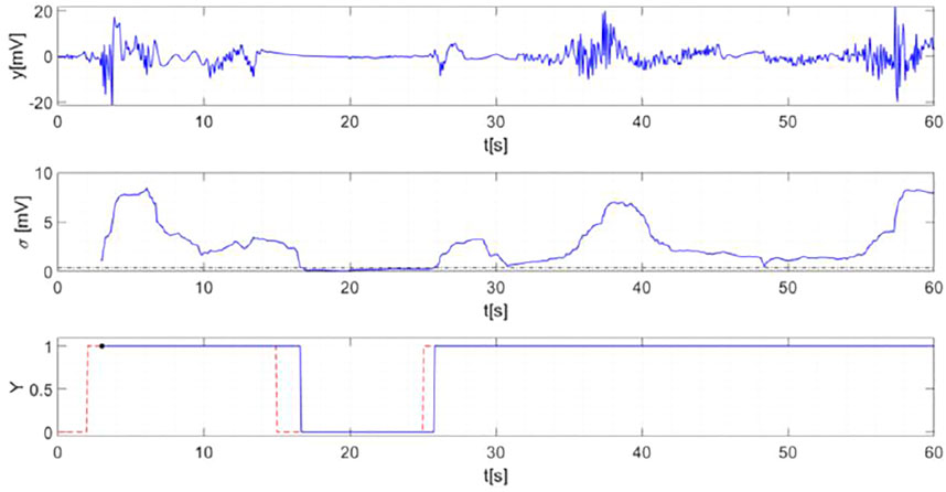
FIGURE 12. Radar signal measured in Test 1 (top panel). Standard deviation (solid line) and optimal threshold γ* (dashed line) (middle panel). SDM output (solid line) compared to ground truth (dashed line).
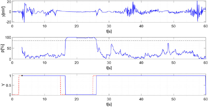
FIGURE 13. Radar signal measured in Test 1 (top panel). Percentage of samples falling in the interval [−
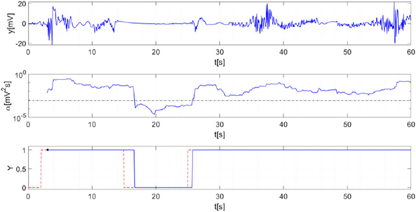
FIGURE 14. Radar signal measured in Test 1 (top panel). Standard deviation (solid line) compared to optimal threshold
In the interval 0–7 s, the subject walks around the room and the signal is quite oscillating. During the interval 7–10 s, the subject stops, then continues to move until t = 15 s when exiting the scene through the corridor. The person stays out the scene for 10 s. Actually, it is easy to observe that the signal is almost flat in the interval 15–25 s. Finally, at t = 25 s, the person re-enters the scene and moves until the end of the acquisition.
The middle panel of Figure 12 shows the real-time standard deviation of radar signal (solid line). As can be seen, the trend of the curve is consistent with radar signal one and remains below the threshold (dashed line) when the scene is empty. The bottom panel of Figure 12 confirms that the output of the detection algorithm (solid line) is in very good agreement with ground truth (dashed line) save for a small time delay occurring in correspondence of the transitions between two different situations in the scene (e.g., the person exits or enters the scene). Such a delay is an effect of the mobile window because it is necessary to accumulate enough samples to detect abrupt variations in the scene. It has been found experimentally that the delay is in the order of half window length, i.e. 1.5 s. The DR obtained in this case is equal to 98.67%, and the failure to reach 100% is only due to the aforementioned delay rather than to erroneous detections.
The results reported in Figure 13 concern the HM and, as observed in the middle panel, the percentages of samples falling in the interval [−0.56, 0.56] mV is higher than the threshold
Figure 14 is concerned with the results achieved by applying DSEM. As expected, the weighted energy of Doppler spectrum overcomes the threshold
For sake of brevity, we do not show the figures of the results related to the Test 2, 3, 4. Nevertheless, Table 3 summarizes the detection performance of each detection strategy for every test.
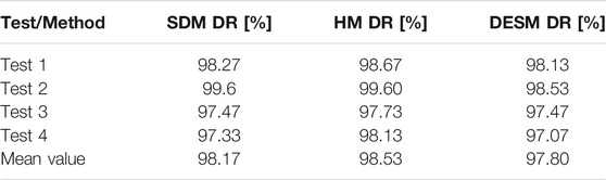
TABLE 3. Testing phase. DR and mean values for SDM, HM, DESM achieved with Test 1, 2, 3, 4 performed in Environment 1.
4.4 Experimental Assessment—Environment 2
Further experiments have been carried out in Environment 2 (see Figure 5). The sensor was recalibrated in this environment by processing novel datasets as done for Environment 1. After system calibration, the following tests were performed:
• Test 5: two male subjects in the scene
• Test 6: one female subject in the scene
• Test 7: two female subjects in the scene
• Test 8: a female and two male subjects in the scene
The tests were performed with the subjects doing analogous activities to those carried out in Environment 1. Table 4 summarizes the test DRs achieved after comparing the detection outputs with the ground truth recorded by the video camera. It can be noticed that satisfactory and consistent DR values are found also for these tests.
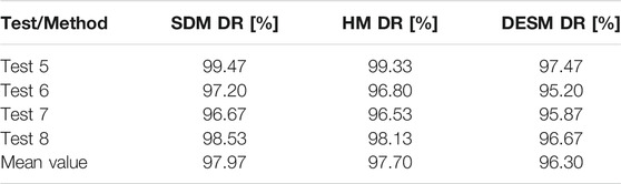
TABLE 4. Testing phase. DR and mean values for SDM, HM, DESM achieved with Test 5, 7, 7, 8 performed in Environment 2.
Based on the data reported in Tables 3, 4, it is natural to wonder why slightly different DR values are obtained for the same test when using different detection strategies. These small percentage differences are attributable not to missed detection or false alarms but rather to the time required by the algorithm to reach the threshold. Indeed, the three techniques share the use of a sliding window that, as seen, introduces a processing delay. It has been found that DSEM takes a slightly longer time to follow abrupt transitions in the scene and, for this reason, it provides on average slightly lower DR values. However, the three procedures can be considered equivalent from a practical viewpoint as the mean DR values achieved by each strategy differ by about one percentage point at most.
As regards the computation complexity, the SDM, HM and DESM take about 1 ms, 1.2 and 2 ms, respectively, to produce a detection. The lower computation time of SDM is expected since it involves simply the calculation of the standard deviation of the windowed signal rather than a histogram or a spectrogram. Nevertheless, all processing delays are small enough to be compliant with real-time operation.
4.5 Robustness Analysis
In all the tests so far described, the SDM, HM, and DSEM detection thresholds were determined from calibration datasets collected in the same environment where the tests were carried out. In the following, we assess the performance of the detection strategies when the detection thresholds are derived from calibration datasets recorded in an environment different from that used for the tests. In other words, the goal is to investigate whether the sensor requires a new calibration every time it is installed in a new environment.
Table 5 lists the DR values related to the tests carried out in Environment 1 when using the thresholds achieved with the calibration performed in Environment 2. Similarly, Table 6 reports the DR values of the tests in Environment 2 when using the thresholds provided by calibration in Environment 1. Upon comparing Table 3 with Table 5 and Table 4 with Table 6, a slight worsening of detection performance is generally achieved when the detection thresholds refer to an environment different from that used for the tests. This outcome is better understood by analyzing the detection thresholds reported in Table 2. As formerly noticed, the higher thresholds of Environment 2 suggest that this environment is noisier and, consequently, using the lower thresholds of Environment 1 in Environment 2 can arise more false alarms, e.g. the radar is able to detect human presence beyond the plasterboard walls. Similarly, applying higher thresholds of Environment 2 in Environment 1 can lead to missed detections as in the case of a stationary person very far from the radar.
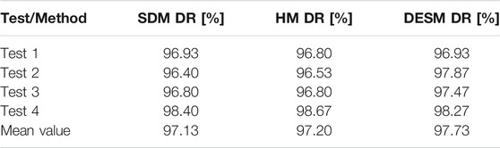
TABLE 5. Testing phase. DR and mean values for SDM, HM, DESM achieved with Test 1, 2, 3, 4 performed in Environment 1 with detection thresholds of Environment 2.
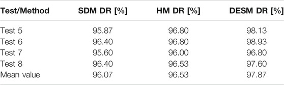
TABLE 6. Testing phase. DR and mean values for SDM, HM, DESM achieved with Test 5, 6, 7, 8 performed in Environment 2 with detection thresholds of Environment 1.
Finally, we analyze also the performance of the three detection strategies when the calibration procedure exploits all twelve datasets (six in Environment 1 and six in Environment 2) simultaneously. To this end, Tables 7, 8 report the average DRs for the trials performed in Environment 1 and 2, respectively, as a function of the calibration type. The data suggest that using more calibration datasets collected in several environments yields intermediate or slightly superior average detection rates compared to those achieved when using the calibration datasets of a single environment. Accordingly, performing a multi-environment calibration appears to be a good practice to enhance the sensor reliability when monitoring different indoor scenarios.
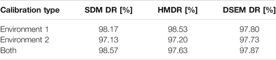
TABLE 7. Testing phase. Mean value of DR for tests performed in Environment 1 versus calibration type.
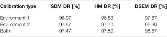
TABLE 8. Testing phase. Mean value of DR for tests performed in Environment 2 versus calibration type.
5 Conclusion
This paper has presented three signal processing strategies for real-time occupancy sensing in indoor environments applied to process data acquired by a continuous wave Doppler radar. A compact prototype has been employed to achieve the goal and a performance assessment of three detection strategies has been performed through experimental trials. As revealed by the tests, all the considered strategies turn out to be very effective both in terms of detection accuracy and computation complexity. In light of the achieved results, CW radar turns out to be a suitable technological solution that may be conveniently integrated with other types of sensors to enhance the reliability of presence detection systems. Future research activity will consider an extensive sensitivity analysis of the detection strategies with respect to the adopted calibration datasets, the effect of the slow drift in the baseband signal and the validation of the prototype at lower power levels. Moreover, the integration of the proposed signal processing algorithms to increase further the reliability of the radar sensor will be also addressed.
Data Availability Statement
The raw data supporting the conclusion of this article will be made available by the authors, without undue reservation.
Author Contributions
Conceptualization, GG, VC, CN, FS, and IC; methodology, GG, VC, CN, FS, and IC, software, GG, VC, and CN; validation, GG, VC, CN, SP, and IC; investigation, GG and IC; writing, GG, VC, CN, SP, FS, and IC. All authors have read and agreed to the published version of the manuscript.
Conflict of Interest
The authors declare that the research was conducted in the absence of any commercial or financial relationships that could be construed as a potential conflict of interest.
Publisher’s Note
All claims expressed in this article are solely those of the authors and do not necessarily represent those of their affiliated organizations, or those of the publisher, the editors and the reviewers. Any product that may be evaluated in this article, or claim that may be made by its manufacturer, is not guaranteed or endorsed by the publisher.
References
Aguasca, A., Acevo-Herrera, R., Broquetas, A., Mallorqui, J., and Fabregas, X. (2013). ARBRES: Light-Weight CW/FM SAR Sensors for Small UAVs. Sensors 13, 32043216–3216. doi:10.3390/s130303204
Ahmad, J., Larijani, H., Emmanuel, R., Mannion, M., and Javed, A. (2021). Occupancy Detection in Non-residential Buildings – A Survey and Novel Privacy Preserved Occupancy Monitoring Solution. Appl. Comput. Inform. 17 (279), 295. doi:10.1016/j.aci.2018.12.001
Alekhin, M., Anischenko, L., and Tataraidze, A. (2013). A Novel Method for Recognition of Bioradiolocation Signal Breathing Patterns for Noncontact Screening of Sleep Apnea Syndrome. Int. J. Antennas Propagation 8, 603. doi:10.1155/2013/969603
Anishchenko, L., Gennarelli, G., Tataraidze, A., Gaysina, E., Soldovieri, F., and Ivashov, S. (2015). Evaluation of Rodents' Respiratory Activity Using a Bioradar. IET Radar, Sonar & Navigation 9, 12961302–1302. doi:10.1049/iet-rsn.2014.0553
Baboli, M., Singh, A., Soll, B., Boric-Lubecke, O., and Lubecke, V. M. (2015). Good Night: Sleep Monitoring Using a Physiological Radar Monitoring System Integrated with a Polysomnography System. IEEE Microw. Mag. 16 (34), 41. doi:10.1109/mmm.2015.2419771
Cerasuolo, G., Petrella, O., Marciano, L., Soldovieri, F., and Gennarelli, G. (2017). Metrological Characterization for Vital Sign Detection by a Bioradar. Remote Sensing 9, 996. doi:10.3390/rs9100996
Chao, C. H., Hsu, T. W., and Tseng, C. H. (2015). Giving Doppler More Bounce: A 5.8 GHz Microwave High-Sensitivity Doppler Radar System. IEEE Microwave Mag. 17 (52), 57. doi:10.1109/MMM.2015.2487919
D.P.C.M. 8/7/, (2003). Decree Defining Exposure Limits, Reference Values and Quality Objectives Protecting the Population from Electric, Magnetic and Electromagnetic fields Produced at Frequencies from 100 kHz to 300GHz.
Dremina, M. K., and Anishchenko, L. N. (2016). Contactless Fall Detection by Means of CW Bioradar.”in Progress in Electromagnetic Research Symposium (PIERS). IEEE. doi:10.1109/piers.2016.7735154
Droitcour, A. D., Boric-Lubecke, O., Lubecke, V. M., Lin, J., and Kovacs, G. T. (2004). Range Correlation and I/Q Performance Benefits in Single-Chip Silicon Doppler Radars for Noncontact Cardiopulmonary Monitoring. IEEE Trans. Microwave Theor. Tech. 52 (838), 848. doi:10.1109/tmtt.2004.823552
EPRI (1994). Occupancy Sensors: Positive On/off Lighting Control. Palo Alto, CA, USA: ” Electr. Power Res. Inst.Rep. EPRIBR-100323.
Esposito, C., Natale, A., Palmese, G., Berardino, P., Lanari, R., Perna, S., et al. (2020). “On the Capabilities of the Italian Airborne FMCW AXIS InSAR System,” in Remote Sensing Microwave engineering (New York: John Wiley &sons), 12, 539. doi:10.3390/rs12030539
Fernández, J. R. M., and Anishchenko, L. (2018). Mental Stress Detection Using Bioradar Respiratory Signals. Biomed. signal Process. Control 43 (244), 249. doi:10.1016/j.bspc.2018.03.006
Geisheimer, J. L., Marshall, W. S., and Greneker, E. (2001). “A Continuous-Wave (CW) Radar for Gait Analysis,” in Proceedings of the IEEE Thirty-Fifth Asilomar Conference on Signals, Systems and Computers, Pacific Grove, CA, USA. doi:10.1109/acssc.2001.987041
Gennarelli, G., Ludeno, G., and Soldovieri, F. (2016). Real-time through-wall Situation Awareness Using a Microwave Doppler Radar Sensor. Remote Sensing 8, 621. doi:10.3390/rs8080621
Hornsteiner, C., and Detlefsen, J. (2008). Characterisation of Human Gait Using a Continuous-Wave Radar at 24 GHz. Adv. Radio Sci. 6, 67–70. doi:10.5194/ars-6-67-2008
Li, C., Cummings, J., Lam, J., Graves, E., and Wu, W. (2009). Radar Remote Monitoring of Vital Signs. IEEE Microwave Mag. 1047 (1), 56. doi:10.1109/mmm.2008.930675
Li, C., Lubecke, V. M., Boric-Lubecke, O., and Lin, J. (2013). A Review on Recent Advances in Doppler Radar Sensors for Noncontact Healthcare Monitoring. IEEE Trans. Microwave Theor. Techn. 61, 2046–2060. doi:10.1109/tmtt.2013.2256924
Lin, J. C. (1979). Microwave Apexcardiography. IEEE Trans. Microw. Theor. Tech. 27 (618), 620. doi:10.1109/tmtt.1979.1129682
Lin, J. C. (1975). Non-invasive Microwave Measurement of Respiration. Proc. IEEE 63, 557–565. doi:10.1109/proc.1975.9992
Lubecke, V. M., Boric-Lubecke, O., Host-Madsen, A., and Fathy, A. E. (2007). Through-the-wall Radar Life Detection and Monitoring. ProcIEEE/MTT-S International Microwave Symposium, 769–772. doi:10.1109/mwsym.2007.380053
Meta, A., Hoogeboom, P., and Ligthart, L. P. (2007). Signal Processing for FMCW SAR. IEEE Trans. Geosci. Remote Sensing 45, 35193532–3532. doi:10.1109/tgrs.2007.906140
Otero, M. (2005). Application of a Continuous Wave Radar for Human Gait Recognition. Proc. SPIE 5809, 538–548. doi:10.1117/12.607176
Tang, H. J., Kaur, S., Fu, L., Yao, B. M., Li, X., Gong, H. M., et al. (2014). Life Signal Detection Using an On-Chip Split-Ring Based Solid State Microwave Sensor. Appl. Phys. Lett. 105, 133703. doi:10.1063/1.4897220
Wang, J., Wang, X., Zhu, Z., Huangfu, J., Li, C., and Ran, L. (2013). 1-D Microwave Imaging of Human Cardiac Motion: An Ab-Initio Investigation. IEEE Trans. Microwave Theor. Techn. 61, 2101–2107. doi:10.1109/tmtt.2013.2252186
Yatman, G., Üzumcü, S., Pahsa, A., and Mert, A. A. (2015). Intrusion Detection Sensors Used by Electronic Security Systems for Critical Facilities and Infrastructures: a Review. WIT Trans. Built Environ. 151 (131), 141. doi:10.2495/safe150121
Keywords: CW radar, Doppler effect, human detection algorithm, indoor environments, occupancy sensing
Citation: Gennarelli G, Colonna VE, Noviello C, Perna S, Soldovieri F and Catapano I (2022) CW Doppler Radar as Occupancy Sensor: A Comparison of Different Detection Strategies. Front. Sig. Proc. 2:847980. doi: 10.3389/frsip.2022.847980
Received: 03 January 2022; Accepted: 31 January 2022;
Published: 02 March 2022.
Edited by:
Shekh Md Mahmudul Islam, University of Dhaka, BangladeshReviewed by:
Nunzia Molinaro, Campus Bio-Medico University, ItalyAditya Singh, KinetiCor, United States
Copyright © 2022 Gennarelli, Colonna, Noviello, Perna, Soldovieri and Catapano. This is an open-access article distributed under the terms of the Creative Commons Attribution License (CC BY). The use, distribution or reproduction in other forums is permitted, provided the original author(s) and the copyright owner(s) are credited and that the original publication in this journal is cited, in accordance with accepted academic practice. No use, distribution or reproduction is permitted which does not comply with these terms.
*Correspondence: Ilaria Catapano, Y2F0YXBhbm8uaUBpcmVhLmNuci5pdA==