 William Ravenscroft
 Stefan Goetze
 Thomas Hain
- Department of Computer Science, The University of Sheffield, Sheffield, United Kingdom
Separation of speech mixtures in noisy and reverberant environments remains a challenging task for state-of-the-art speech separation systems. Time-domain audio speech separation networks (TasNets) are among the most commonly used network architectures for this task. TasNet models have demonstrated strong performance on typical speech separation baselines where speech is not contaminated with noise. When additive or convolutive noise is present, performance of speech separation degrades significantly. TasNets are typically constructed of an encoder network, a mask estimation network and a decoder network. The design of these networks puts the majority of the onus for enhancing the signal on the mask estimation network when used without any pre-processing of the input data or post processing of the separation network output data. Use of multihead attention (MHA) is proposed in this work as an additional layer in the encoder and decoder to help the separation network attend to encoded features that are relevant to the target speakers and conversely suppress noisy disturbances in the encoded features. As shown in this work, incorporating MHA mechanisms into the encoder network in particular leads to a consistent performance improvement across numerous quality and intelligibility metrics on a variety of acoustic conditions using the WHAMR corpus, a data-set of noisy reverberant speech mixtures. The use of MHA is also investigated in the decoder network where it is demonstrated that smaller performance improvements are consistently gained within specific model configurations. The best performing MHA models yield a mean 0.6 dB scale invariant signal-to-distortion (SISDR) improvement on noisy reverberant mixtures over a baseline 1D convolution encoder. A mean 1 dB SISDR improvement is observed on clean speech mixtures.
1 Introduction
Signal enhancement of speech signals recorded in far-field scenarios has been active research topic for some decades now (Benesty, 2000; Cauchi et al., 2015; Reddy et al., 2021). Isolating individual speakers from signal mixtures is often necessary when applying speech processing systems in real life applications (Wang and Chen 2018; Haeb-Umbach et al., 2021). Speech separation is a common approach to solving this problem. While there has been significant progress in recent years using deep neural network based architectures to separate clean speech mixtures (Luo et al., 2017; Shi and Hain, 2021), the performance still drops significantly in noisy environments, especially for low signal-to-noise ratios (SNRs) (Wichern et al., 2019; Cosentino et al., 2020; Maciejewski et al., 2020). Early approaches for separating speech signals were based on harmonic relationships in the signal (Parsons, 1976) or non-negative matrix factorization (NMF) (Schmidt and Olsson, 2006; Cauchi et al., 2016) and later deep neural network (DNN) variations on NMF approaches (Le Roux et al., 2015; Moritz et al., 2017).
Models that used learned filterbank transforms from the time domain such as TasNets are able to consistently outperform models based on short-time Fourier transform (STFT) features (Luo and Mesgarani, 2018; Luo and Mesgarani, 2019; Luo et al., 2019; Chen et al., 2020; Ochiai et al., 2020; Subakan et al., 2021). The encoder of TasNets can be interpreted as filter banks and this paper aims at visualising the encoded signals in TasNets in that respect. Luo and Mesgarani, (2018) first proposed a recurrent TasNet (BLSTM-TasNet) model composed of a 1-dimensional convolutional encoder, bidirectional long short term memory (BLSTM) masking network and a transposed 1-dimensional convolutional decoder. Luo and Mesgarani, (2019) revised this into a fully convolutional network (Conv-TasNet) by replacing the BLSTM network with a temporal convolutional network (TCN) (Lea et al., 2016). Shi et al. (2019) proposed the introduction of gating mechanisms into the TCN as a means of controlling the flow of information through the network. A dual path recurrent neural network model (DPRNN) was introduced by Luo et al., (2019) which reorganises the input data into multiple data chunks and processes the inter chunk and intra chunk data sequentially using an long short term memory (LSTM) based network for modelling temporal context in sequences. The dual path Transformer network (DPTNet) (Chen et al., 2020) and Sepformer (Subakan et al., 2021) are dual path models that replace the recurrent neural networks in the DPRNN model with Transformer networks (Vaswani et al., 2017; Katharopoulos et al., 2020) for modelling temporal context in the mask estimation part of the network. Work by Kadıoğlu et al. (2020) focused more on the encoder and decoder part of the generalized TasNet model structure where a deeper convolutional encoder and decoder network were proposed for the Conv-TasNet model. It was shown by Yang et al. (2019) that combining the learned features of Conv-TasNet’s encoder with STFT features leads to a small improvement performance for clean speech separation tasks. Similarly, Pariente et al. (2020) demonstrated that using complex-valued learnable analytic filterbanks in the encoder and decoder can lead to further performance improvement over real valued encoder of Conv-TasNet. Ditter and Gerkmann, (2020) proposed hand-crafted multi-phase gammatone (MPGT) filter bank features over the learned filterbank in Conv-TasNet. This approach was effective when just applied to the encoder but the learned decoder of Conv-TasNet proved more effective than their MPGT based decoder.
This work investigates the use of attention mechanisms in the encoder and decoder of TasNets to improve the performance, particularly in noisy and reverberant situation. Vaswani et al. (2017) proposed MHA as a way to parallelize a single attention mechanism into multiple attention heads while maintaining a similar parameter count to single headed attention. This work proposes incorporating multihead attention mechanisms into the encoders and decoders of Conv-TasNet to improve the performance on noisy and reverberant speech mixtures where it is assumed that the noisy content of the data is orthogonal to the speech. Some discussion about the relevance of the orthogonality assumption and its relationship to cross correlation is given to motivate why attention mechanisms are a suitable choice for improving the encoders and decoders. The network structures are evaluated on noisy and reverberant data from the WHAMR corpus (Maciejewski et al., 2020). Although the main goal of this work is to minimize the negative effects of additive noise under the assumption of orthogonality, separation of reverberant speech mixtures, i.e. with convolutive noise (reverberation) are also considered. The remainder of this work proceeds as follows. In Section 2 the Conv-TasNet model is briefly revised and analyzed. In Section 3 the proposed Multihead Attention and the novel encoder and decoder structures are introduced. The training configuration and experiments conducted on the WHAMR corpus are explained in Section 4. Further discussion and some conclusions are give in Section 5.
2 Conv-TasNet
In this section the Conv-TasNet speech separation network proposed by Luo and Mesgarani, (2019) is reviewed. The network is composed of three components: an encoder, a mask estimation network and a decoder. A schematic of the network structure is shown in Figure 1 exemplary for C = 2 output signals. The mask estimation network formulated in this section follows the implementation that can be found in the open source SpeechBrain Ravanelli et al. (2021) and ESPnet (Li et al., 2021) software toolkits. This implementation differs slightly from the original proposed by Luo and Mesgarani, (2019) which is discussed in greater detail in Section 2.3.
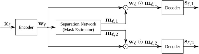
FIGURE 1. Generalised TasNet Model Schematic (exemplary shown for two speakers, C=2).
2.1 Signal Model and Problem Formulation
The problem of monaural noisy reverberant speech separation is a 1 dimensional additive and convolutive problem for which the microphone signal
The symbol * in (1) denotes the convolution. The aim implicit in the noisy reverberant speech separation task is to find C estimates for each of sc(t), denoted as
The discrete mixture x [i] is processed in overlapping segments of length LBL such that:
where ℓ is the frame number for each of Lx frames and
The encoder encodes short overlapping blocks of the time domain signal xℓ as defined in (2). The encoder is a convolutional neural network where the layer weights are learned in an end-to-end (E2E) fashion. The mask estimation takes the output of the encoder network wℓ and uses it to estimate a set of mask-like vectors mℓ,c for each of the C speakers. These mask-like vectors are then multiplied with the encoded signal vector wℓ, producing a masked weight vector for each speaker. The decoder in the original Conv-TasNet approach (Luo and Mesgarani, 2019) is a transposed 1D convolutional layer that decodes these representations back into the time domain to result in C separated source estimates
2.2 Encoder
The first stage of the network is to encode the input audio. The encoder is a constructed using a 1D convolutional filter of kernel size LBL with 1 input channel and N filters and an optional nonlinear encoder activation layer denoted by
where
2.2.1 Channel Sorting for Visualisation of Encoded Signals
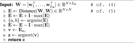
While time-frequency approaches for speech separation based on masking spectrogram representations are often easy to interpret, for visualization of the encoded signal W, sorting over the output convolutional channels n is beneficial. When visualising the encoded representations in this work, the encoded signals’ channels are thus reordered according to the sorting algorithm defined in Algorithm 1 based on depthwise Euclidean distance. In the Conv-TasNet paper, Luo and Mesgarani, (2019) propose using unweighted pair group method with arithmetic mean (UPGMA) to sort the channels by Euclidean filter similarity. The proposed Algorithm 1 was found to be preferable in many cases to Luo and Mesgarani, (2019)’s approach as it leads to a less granular representation with most of the speech energy being located in the lower region of the representation, making it easier to observe lower energy noisier regions within the encoded signal. Consequently, the proposed channel sorting algorithm results in visualisations more similar to well-known spectrogram-like time-spectral representations. The key difference of the proposed sorting algorithm is that Luo and Mesgarani, (2019)’s method uses filter similarity to sort channels whereas the proposed method sorts channels according to encoded feature similarity. The use of UPGMA which is based on a clustering approach to sort the channels is also not clearly motivated by Luo and Mesgarani, (2019) hence in our approach we simply suggest sorting the channels by decreasing similarity from the most similar channels measured in Euclidean feature similarity. This is premised on the assumption that the most similar channels will contain the most amount of speech energy.
Algorithm 1. Channel sorting algorithm.
The distance matrix E in line 1 of Algorithm 1 is composed of Euclidean distances between the encoded channel representations, calculated element-wise by
with
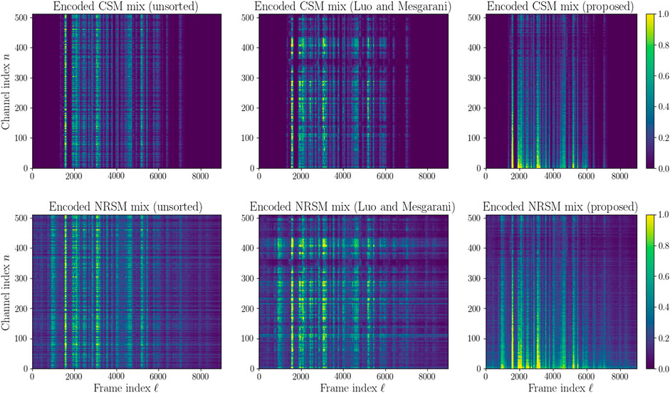
FIGURE 2. Encoded signal matrix W for clean speech mixtures (CSM) (top) and noisy reverberant speech mixture (NRSM) (bottom). From left to right: unsorted; sorted using Luo and Mesgarani, (2019)’s method; sorted using the proposed method in Algorithm 1.
2.3 Mask Estimation Network
The separation network is visualised in Figure 3. It uses a TCN which consists of X layers of convolutional blocks (horizontal and coloured in Figure 3A) which are repeated R times (vertical in Figure 3A). The initial channel-wise normalisation for each block of the encoded signal wℓ is defined as
where
FIGURE 3. (A) Temporal Convolutional Mask Estimation Network. (B) Network layers inside ConvBlock in Figure 3A.
2.3.1 Convolutional Blocks
Each of the convolutional blocks consist of a pointwise 1D convolutional layer proceeded by a depthwise separable convolutional operation as visualized in Figure 3B resulting in H channels within the convolutional block. Each subsequent convolutional block has an increasing dilation factor f = 20, 21, …, 2X−1 which widens the temporal context of the network for every additional block. This implementation of the Conv-TasNet TCN follows that which is used in popular research frameworks such as SpeechBrain (Ravanelli et al., 2021) and ESPnet (Watanabe et al., 2018; Li et al., 2021). This implementation is in contrast to the original Conv-TasNet proposed by Luo and Mesgarani, (2019) which includes an additional skip connection from a parallel convolutional layer at the output of the convolutional blocks.
Conv-TasNet was originally proposed in both causal and non causal implementations. In the causal implementation cumulative layer normalization is proposed by Luo and Mesgarani, (2019) for the normalization layers in the convolution blocks. In the implementations and results in following sections the focus is on the non-causal model which utilises global layer normalization (gLN) for normalizing intermediate layers inside the convolutional blocks. The gLN function is defined as
where
A parametric ReLU (PReLU) activation function is used after the initial pointwise convolution as well as the in the depthwise separable convolution, denoted by
The depthwise separable convolution is an efficient algorithm for computing convolutions where the convolution is computed in two stages:
1) In the first stage a depthwise convolution, i.e. a convolution per channel, is applied to each of G input channels.
for the input matrix
2) In the second stage pointwise convolution is then performed across each of the H channels. This operation is defined as
where
The depthwise separable convolution operation has G × P + G × H parameters where as standard convolution operation has G × P × H which means that the model size is reduced by a factor of
2.3.2 Temporal Context
The TCN has a fixed window of depthwise inputs that the output layer is able to observe for a given output block. This window of data points is of interest particularly as the input speech data to the network can be modelled as a causal system with long term dependencies particularly with reverberant speech signals for which the room impulse response hc(t) in (1) significantly increases long term dependencies. The receptive field of a convolutional network refers to the number of data points that can be simultaneously observed by the network at the final convolutional layer in a deep convolutional network. The receptive field for the temporal convolutional network (TCN) used in Conv-TasNet depends on the number of convolutional blocks defined by blocks repetitions X and R as well as the kernel size P and can be defined as
The receptive field in (15) is measured in the number of frames observed in a given sequence. When the entire Conv-TasNet model is considered, it is possible to use the receptive field to measure the total temporal context observed by the whole network at any given output, measured in seconds. Given the sample rate fs and the block size LBL, the receptive field in seconds is
2.3.3 Output Masks
The output features of the TCN network for each frame ℓ are a concatenated vector of estimated masks, which is defined as
where
2.4 Decoder
The input signal of the decoder U is an element-wise multiplication of the masks mℓ,c and the encoded mixture wℓ from (3). Estimates for the source signals
where
However, no restraints are put on the model training to enforce this condition so that this only assists the understanding in how the model is expected to learn and hence can be a useful approach in interpreting the model.
2.5 Objective Function
The objective function used for training is scale-invariant signal-to-distortion ratio (SISDR)
which is a commonly used objective function for training DNN speech separation systems (Luo and Mesgarani, 2018; Luo and Mesgarani, 2019; Luo et al., 2019; Chen et al., 2020; Subakan et al., 2021), sometimes with minor modifications.
in (21) is the scale invariant target speech and
the residual distortion present in the estimated speech. The clean speech segment is denoted by
2.6 Deep PReLU Encoders and Decoders
Some work has already been done to investigate improved encoders and decoders for the Conv-TasNet model. Deeper convolutional encoder and decoder networks were proposed by Kadıoğlu et al. (2020) for use with Conv-TasNet on speech separation tasks. In this work, this deep convolutional encoder and decoder model is implemented as an additional baseline to the original Conv-TasNet model described in the previous part of this section. The deep convolutional encoder consists of three additional 1D convolutional layers each with the a kernel size of three and a stride of 1. Each convolutional layer is proceeded by a PReLU activation function. The number of input and output channels are equal to N. Their deep convolutional decoder is similarly constructed of an additional three transposed 1D convolutional layers proceeded by PReLU activation functions. Each additional transposed 1D convolutional layer has the same kernel size and stride as the additional encoder layer. Each layer also has N input and output channels. It was found by Kadıoğlu et al. (2020) that increasing the dilation of the encoder and decoder layers had negligible effects on the SISDR separation performance and so a fixed dilation of 1 is used for each layer.
3 Multihead Attention Encoder and Decoders
In the following, the proposed MHA encoder and decoder designs are introduced. The scaled dot product attention function (Vaswani et al., 2017) and MHA are briefly introduced and the proposed application of MHA in the TasNet architecture is described. Attention was first proposed by Bahdanau et al. (2015) as a layer in DNN models that can be used to asses the similarity or relevance between two sets of features and thus provide attention to more relevant features.
3.1 Attention Mechanism
In this work, scaled-dot product attention
is used where
In the encoders and decoders proposed here, the output of the attention function is used to re-weight a sequence of features according to which features in a sequence have the most pointwise correlation (i.e. correlation across channels as opposed to across discrete time) to one another. There is a twofold assumption in our proposed application of the attention function. The first is that encoded blocks containing speech will have a higher correlation to one another than blocks containing noise. Note that this is a similar assumption to the orthogonality assumption made by Roux et al. (2019) in the SISDR objective function in (21) used for training models in this work. The second assumption is that in the encoded speech mixture of each individual speaker’s speech signal will have a larger pointwise correlation to itself than to any other speaker across all frames.
Figure 4 demonstrates the proposed approach to calculating the self-attention (Lin et al., 2017) of the transposed encoded signal blocks W from (4), i.e. K = Q = V = W⊤. The lower right panel shows then output of the attention mechanism which is then used to re-weight the encoded mixture in the lower left panel.
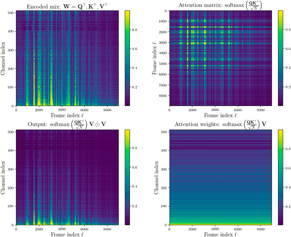
FIGURE 4. Top left: encoded NRSM signal. Top right: Computed attention matrix weights. Bottom right: Scaled dot product attention. Bottom left: encoded NRSM signal re-weighted with attention. The figures on the left have had values above 0.05× their maximum values clipped and are normalized between 0 and 1. The figures on the right are normalized between 0 and 1.
Figure 5 shows the attention weighted encoded input (middle panel) compared to an encoded NRSM features (top panel) as well as the corresponding encoded CSM features (bottom panel). The attention weighting adds greater emphasis to much of the features containing speech and conversely weights down some of the noisier parts of the encoded features.
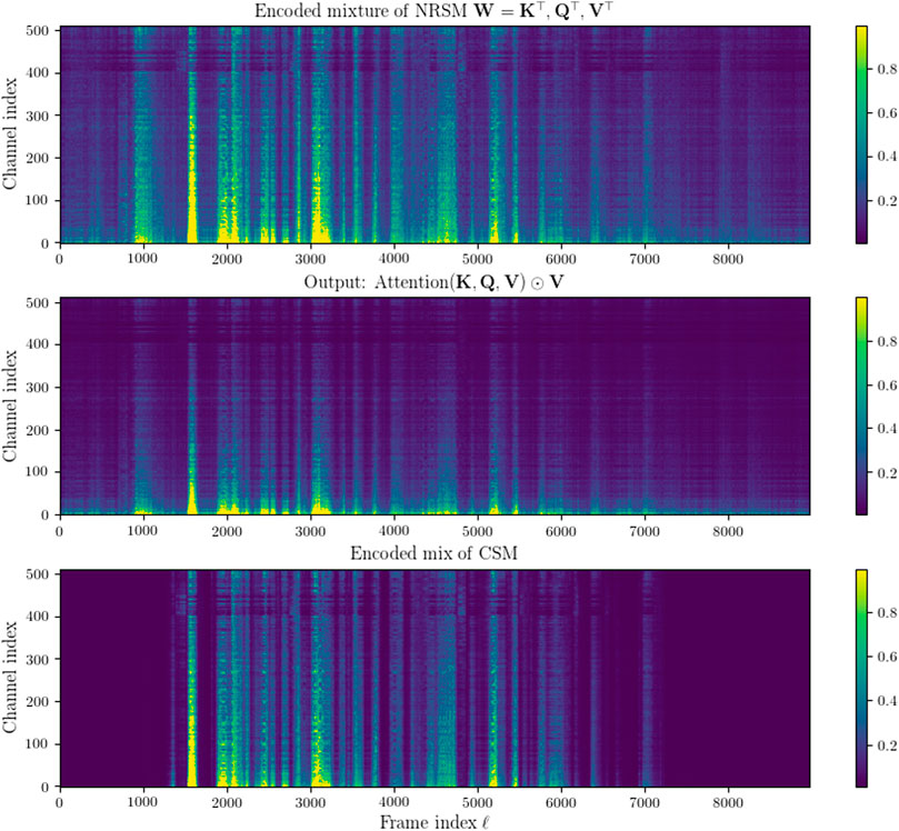
FIGURE 5. Top: Encoded NRSM signal blocks. Middle: Encoded NRSM signal blocks re-weighted with attention as defined in (24). Bottom: Encoded CSM signal blocks (ν(t)=0, hc(t)= δ(t), ∀t ≥0). The top and bottom figures clip values above 0.05× the maximum value of the encoded NRSM signal and then normalized between 0 and 1. The middle figure clips values above 0.05× its maximum value and is then normalized between 0 and 1.
3.2 Multihead Attention Layer
The following section introduces multihead attention (Vaswani et al., 2017) as an extension to scaled dot product attention within the context of the encoder and decoder model proposed in this work where all the inputs to the attention layer are of equal dimensions.
3.2.1 Linear Projections and Attention Heads
To simplify notation in the following model descriptions, V, K,
for each attention head a ∈ {1, … , A} where A is the number of attention heads and d = N/A is the reduced dimensionality. The motivation for reducing the dimensionality is that this retains roughly the same computational cost of using a single attention head with full dimensionality while allowing for using multiple attention mechanisms. Each of these weight matrices are used to compute (Ka, Qa, Va) for each attention head a ∈ {1, … , A} such that
For each attention head the attention function is computed such that
where χa is the ath attention head.
3.2.2 Multihead Attention
The final stage is connecting the attention heads by concatenating a long the d length dimension and projecting the features using a linear layer defined by a weight matrices
The combined concatenation and linear projection is defined by the Multihead Attention function
3.2.3 MHA Encoder and Decoder Architectures
In this section the MHA encoder and decoder architectures are described. Both the encoder and decoder models use a similar paradigm by applying a multihead attention layer followed by a non-linearity to produce a set of mask like features which are then used to weight and encoded mixture.
3.2.3.1 Encoder
For the encoder self-attention (Lin et al., 2017) is used. self-attention refers to applying attention across a sequence to itself. Therefore the inputs to the MHA layer are defined as visualized in Figure 6 such that
where every input to the MHA layer is the encoded mixture from a 1D convolutional layer and ReLU activation similarly as in (3). The output of the MHA layer is then treated in a mask-like fashion where it is multiplied element-wise with the encoded mixture. This representation is then proceeded by a ReLU activation. Empirically it was found that placing the ReLU activation after the elementwise multiplication as opposed to using the direct output of the MHA layer consistently yield better performance across all acoustic conditions. The complete network diagram for the MHA encoder is shown in Figure 6.
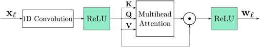
FIGURE 6. Convolutional MHA encoder diagram.
3.2.3.2 Mask Refinement and Post-Masking Decoders
A number of approaches are proposed. Two encoder-decoder attention (Vaswani et al., 2017) based decoder models are proposed in the following subsection. The first is referred to as mask refinement (MR) and the other is referred to post-masking (PM). Both decoders are composed of an MHA layer proceeded by a ReLU activation function and a transposed 1D convolutional layer. For both architectures the input to the MHA layers are defined as
where c ∈ {1, … , C} and C is the number of target signals. These inputs are defined to combine the principles of encoder-decoder attention, described in Section 3.2.3 of Vaswani et al. (2017), with those of self-attention as both the key and query contain information from the estimated masks. The same MHA layer is used for each speaker.
The MR decoder produces a mask from the MHA layer proceeded by a ReLU function which is multiplied by the encoded mixture and this re-masked encoded mixture is then decoded back into the time domain with the transposed 1D convolutional layer. The MR decoder model is depicted in Figure 7A. The motivation in this design is to use the MHA mechanism to produce a mask that refines the already masked encoded representation such that is attends better to features most relevant to the most present speaker features in the original masked encoded features.

FIGURE 7. (A) MHA mask refinement (MR) decoder architecture. (B) MHA post-masking (PM) decoder architecture. (C) MHA self-attention (SA) decoder architecture.
The post-masking decoder (PMD) also uses an MHA layer to produce a new mask but in this model the new mask is used to refine the already masked encoded mixture. The PMD model is shown in Figure 7B. The motivation in this design is to use the MHA mechanism to produce a new mask by observing speaker information in the masks and masked encoded mixtures to produce an improved hypothesis of what that masks should be by attending to the most prevalent an correlated speaker information in both types of representation.
3.2.3.3 Self-Attention Decoder
An additional decoder based on self-attention is proposed shown in Figure 7C. This decoder applies MHA to the masks estimated by the network defined in Section 2.3 in a self-attentive manner such that
The output of the MHA layer is proceeded by a ReLU function to produce a new set of masks. The Hadamard product of the new masks with the encoded mixture is then computed. This masked encoded mixture is then decoded back into the time domain using a transposed 1D convolutional layer.
3.3 Relationship Between Dot Product and Cross-Correlation
Some brief discussion is given to how the scaled dot product function in multihead attention can be formulated as computing a cross correlation matrix of finite discrete processes across the features of each frame ℓ. Using this formulation it is suggested that the attention mechanism naturally applies more weight across frames that are highly cross correlated and applies less weight across frames that have lower cross correlation.
The discrete cross-correlation function of two finite processes q [n] and k [n] can be estimated by
The numerator of (24) is the following matrix of size Lq × Lk for which in the following Lq = Lk = Lx.
For each cell in the resultant matrix there is the dot product of the feature vectors qℓ and kℓ which can be written more explicitly as
In Eq. 35,
3.4 Encoder and Decoder Complexities
Some brief discussion is given to the model complexities predominantly for reference. The complexities for each of the proposed encoders and decoders as well as the baselines used later in Section 4 are given in Table 1.
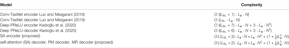
TABLE 1. Complexity of all encoder and decoder models evaluate including all non-linearities, weights and biases.
The proposed encoder described in 3.2.3.1 is more computationally complex than the encoders proposed by Luo and Mesgarani, (2019) and Kadıoğlu et al. (2020) however a significant reason for this is that the attention operation considers the entire sequence length as opposed to operating over a smaller context window as is the case in the other encoders. The same is true of the proposed decoders described in Section 3.2.3.2 and Section 3.2.3.3 compared with the purely convolutional decoders proposed by Luo and Mesgarani, (2019) and Kadıoğlu et al. (2020). In future work, ways to alleviate the computational complexity using linear attention (Katharopoulos et al., 2020) and restricted self-attention (Vaswani et al., 2017) can be explored but this is beyond the scope of the work presented here.
4 Experiments
This section presents details on the experimental setup as well as the results performed to evaluate the proposed encoders and decoders in the previous section.
4.1 Data
A number of datasets have been proposed for benchmarking speech separation systems (Cosentino et al., 2020). The WSJ0-2Mix dataset, published first in Hershey et al. (2016) and Isik et al. (2016), is a popular simulated dataset for clean speech separation. However, it neither includes additional noise nor reverberation as targeted in this work in (1). To incorporate additional noise the (WSJ0 Hipster Ambient Mixtures) WHAM corpus was introduced in Wichern et al. (2019) and to incorporate reverberation effect, the WHAMR dataset was proposed by Maciejewski et al. (2020) as a noisy reverberant extension to WSJ0-2Mix and is used for all experiments in this section. WHAMR is a corpus of noisy reverberant speech mixtures. For each training example there is a mixture and two targets. Speech mixtures are evaluated under four different acoustic conditionss (ACs): CSM, i.e. ν(t) = 0 and h(t) = δ(t) in (1), noisy speech mixture (NSM), i.e. h(t) = δ(t) but noise present in (1), reverberant speech mixture (RSM) i.e. v(t) = 0 but reverberation present in (1), and NRSM. The training set consists of 20,000 training examples resulting in overall 58.03 h of speech, the validation set consists of 5,000 training examples equalling 14.65 h of speech and the test set consists of 3,000 examples resulting in 9 h of speech. 8kHz audio samples are used and clipped to 3 s segments for training. This length constraint is removed for validation and testing.
Noise clips were sampled from a number of urban environments and these are mixed with the speech mixtures at a randomly selected SNR value from a uniform distribution between −6 and +3 dB. RIRs are also randomly generated. An RIR is generated for each speaker from the same simulated room environment. The RIRs have a reverberation time RT60 ranging from 0.1 to 1 s and are generated using the pyroomacoustics software package (Scheibler et al., 2018).
4.2 Training Configuration
The Conv-TasNet model is implemented using the SpeechBrain framework introduced by Ravanelli et al. (2021). The specific model configuration used is slightly different to both WHAMR baselines provided by Maciejewski et al. (2020) as an improved configuration was found. As previously noted, the mask estimation network in SpeechBrain1 neglects the skip connections in the original Conv-TasNet model proposed by Luo and Mesgarani (2019) and implemented in Maciejewski et al. (2020)1. A comparison of the different model parameters as well as the CSM SISDR performance and temporal context, reported in seconds (s), of each network is shown in Table 2.
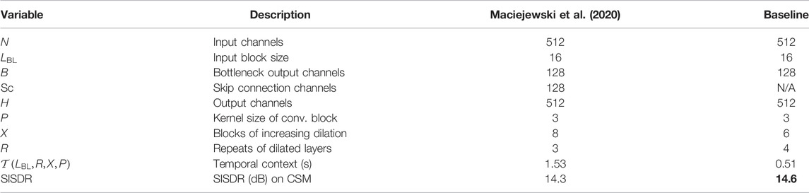
TABLE 2. Details of the Conv-TasNet configuration compared to Maciejewski et al. (2020). Bold indicates SISDR result of the proposed baseline.
An utterance-level permutation invariant training (PIT) scheme (Kolbaek et al., 2017) is employed to deal with the unknown mismatches of the speech separator. An initial learning rate of 1 × 10⁻³ is used and scheduler is used that halves the learning rate if there is no average SISDR improvement of the model for three epochs. A batch size of 4 was used. A total of 100 epochs of training were performed.
4.3 Assessment Metrics
Performance is measured using SISDR, signal-to-distortion ratio (SDR), perceptual evaluation of speech quality (PESQ) and short-time objective intelligibility (STOI).
SDR is a generalized SNR metric that measures the amount of energy in the signal compared with the energy in the combined residual noise, artifacts and interference. SDR has been widely used in assessing source separation models in general (Stoller et al., 2018; Luo and Mesgarani, 2019).
PESQ was proposed by Rix et al. (2001) as an objective measure for speech quality assessment. The design of PESQ is supposed to offer similar results to Mean Opinion Score (MOS) by using psychoacoustically motivated filter models. The measure ranges from −0.5 to 4.5, with −0.5 being considered lowest quality. PESQ is often used for assessing general denoising and dereverberation tasks. It has also been used for assessing speech separation performance (Wang et al., 2014; Deng et al., 2020).
STOI is an intelligibility metric proposed by Taal et al. (2010) which uses correlation ratios between clean and degraded signals to asses the intelligibility of the degraded signal with a score between 0 and 1. STOI has been commonly used for assessing general speech enhancement tasks but has also been used in assessing speech separation models (Deng et al., 2020).
Δ measures are shown in addition to the absolute metric values to indicate the improvement in quality or intelligibility between the noisy reverberant signal mixture x and the network estimates
4.4 Results
The following subsections address the speech separation results of the proposed method in comparison to baseline methods on the WHAMR corpus. The MHA encoder is evaluated first and then two subsequent sections analyse the MHA decoder architectures and look at how the number of attention heads affects performance. All metrics use the permutation invariant training schema to find the optimal value of each metric under the assumption this is the correctly matched permutation of speakers. Every set of results is compared against the original encoder and decoder proposed by Luo and Mesgarani, (2019) reported as Conv-TasNet and the deep convolutional encoder and decoder model proposed by Kadıoğlu et al. (2020) is reported as Deep PReLU.
4.4.1 MHA Encoder Results
The MHA encoder model seen in Figure 6 is compared to the original Conv-TasNet baseline encoder proposed by Luo and Mesgarani, (2019) as well as the Deep PReLU approach proposed by Kadıoğlu et al. (2020). The results for this comparison across all four acoustic conditions can be seen in Table 3. The MHA encoder are denoted as the self-attention encoder (SAE) in all results.

TABLE 3. Comparison of MHA encoder with 4 attention heads to Original Conv-TasNet encoder across various acoustic conditions. Bold indicates the best performing model for each acoustic condition and metric.
These results demonstrate a consistent improvement of the MHA encoder over the original baseline purely convolutional encoder. Highest improvement in performance can be observed for the clean speech mixtures (CSM) since this is the easiest task for the network. The MHA encoder achieved slightly more performance improvement on the RSM condition than the NSM condition and the NRSM. The MHA encoder outperformed the Deep PReLU encoder on every acoustic condition. Figure 8 shows the intermediate features in the MHA encoder encoding an NRSM signal. Comparing the encoded signal after the first convolutional layer in the network to the similar representation in Figure 6 it is notable that the convolutional layer has learned to focus on a narrow set of channels. This implies a large number of the channels are in fact redundant, a similar find to the MPGT encoder and convolutional decoder model proposed by Ditter and Gerkmann, (2020). The final output of the MHA encoder further narrows the focus of the encoded features.
Another interesting finding of the output of the MHA layer is that the mask-like features do not seem to attenuate the signal where there is only noise present as one might expect due noise not being present in the target signal at training. This effect can be seen more clearly when compared to the intermediaries of the CSM signal encoded by the MHA encoder in Figure 9.
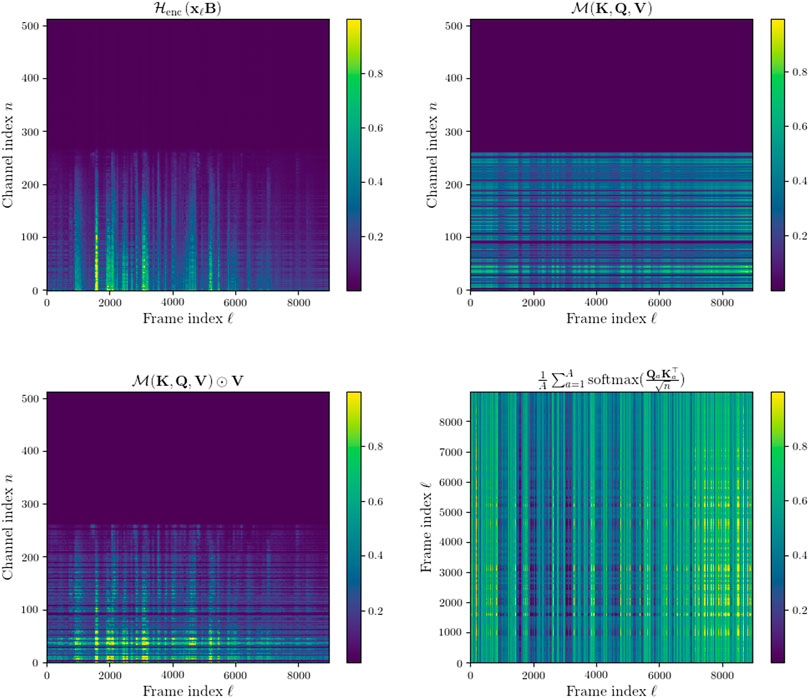
FIGURE 8. Top left: encoded NRSM features after 1D convolution and non-linearity in MHA encoder sorted using Algorithm 1. Top right: mask-like output of self attentive MHA layer in MHA. Bottom left: output of the MHA encoder. Bottom right: Averaged attention weight matrix across all attention heads, A =4.
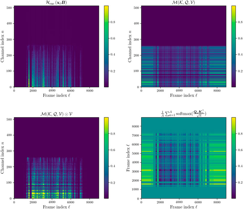
FIGURE 9. Top left: encoded CSM features after 1D convolution and non-linearity in MHA encoder. Top right: mask-like output of self attentive MHA layer in MHA. Bottom left: output of the MHA encoder. Bottom right: Averaged attention weight matrix across all attention heads, A = 4.
4.4.2 MHA Decoder Architecture Comparisons
A comparison of the mask refinement decoder (MRD) in Figure 7A, the PMD in Figure 7B and the self-attention decoder (SAD) in Figure 7C is carried out in the following to analyse which approach, if any, leads to superior decoding performance over the Conv-TasNet baseline (Luo and Mesgarani, 2019) and Deep PReLU decoder (Kadıoğlu et al., 2020). The results are shown in Table 4. In each case the number of attention heads is set to A = 2.

TABLE 4. Comparison of MRD in Figure 7 (a) to PMD in Figure 7 (b) across various acoustic conditions. Bold indicates the best performing model for each acoustic condition and metric.
There was a clear performance improvement on clean speech mixtures across all metrics with the MRD in Figure 7A. Also a noticeable performance increase can be observed for the reverberant speech mixtures but this improvement is not also seen for the noisy reverberant speech mixtures where there was a small drop across all measures except for the STOI measure. The PMD design showed decreased performance across all conditions and metrics. The best performing of the proposed decoders across all conditions was the self-attention decoder. This decoder also outperformed the baseline Deep PReLU decoder with greater success the more challenging the audio became, c. f. SISDR results for CSM, NSM conditions with SISDR results for RSM and NRSM conditions.
4.4.3 MHA Decoder Number of Heads Comparisons
Results shown in Section 4.4.2 demonstrated that the proposed self-attention decoder in Figure 7C was more effective than the MR and PM decoders. The MR decoder also showed some potential performance improvement for the CSM condition but this was not replicated across all conditions. In the following subsection, further analysis is done using the SAD and MRD to observe the effect that using a variable number of heads might have on the model. Experiments were performed using A = {2, 4, 8} attention heads for both decoders and are again compared against the Conv-TasNet (Luo and Mesgarani, 2019) and Deep-PReLU baselines (Kadıoğlu et al., 2020).
The results in Table 5 show that using A = 4 attention heads leads to a small but consistent performance increase across all metrics used for MRD over the original Conv-TasNet decoder. The smallest improvement is often close to 0.1 dB SISDR and it is thought that this is not a strong enough improvement beyond the effects of randomized model initialization to confirm that this technique as implemented here is any more effective than the original Conv-TasNet decoder. The SAD again shows consistent improvement over the previously demonstrated model with only two attention heads for both A = 4 and A = 8. Typically for both models A = 4 leads to best average improvement across all metrics for both the MRD and SAD.
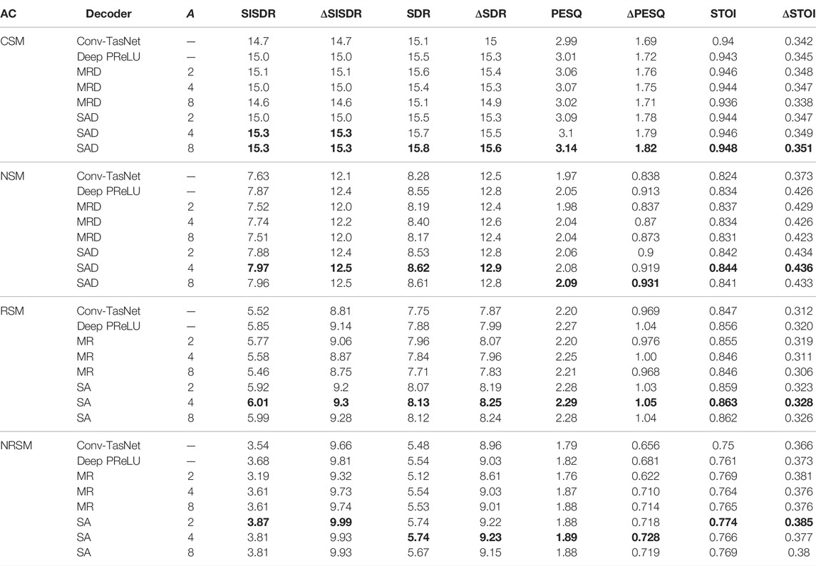
TABLE 5. Comparison of using 2, 4 and 8 attention heads in MRD (Figure 7a) against the original Conv-TasNet decoder proposed by Luo and Mesgarani, (2019). Bold indicates the best performing model for each acoustic condition and metric.
4.4.4 Comparison of Combined MHA Encoder/Decoder Models to Deep Convolutional Encoder/Decoder
The final set of results given in this section compare the MHA encoder and decoder approach to a deep convolutional encoder and decoder proposed by Kadıoğlu et al. (2020). A Conv-TasNet model utilising both the proposed MHA encoder and decoder was trained in an E2E fashion. For all results the SAE, SAD and MRD 4 attention heads were used. Similarly a Conv-TasNet model using both the deep encoder and decoder proposed by Kadıoğlu et al. (2020) was trained. The SAE with the original Conv-TasNet decoder are reported with the decoder abbreviated to convolutional decoder (CD) for brevity in some results.
The results in Table 6 show that the proposed combinations of the SAE with the SAD or MRD lead to better results across all metrics for the CSM, RSM and NRSM acoustic conditions compared to the Deep PReLU baseline. The combination of the SAE with both the proposed decoders performed worse in all metrics than the SAE with the original Conv-TasNet decoder. This implies again that the minimal performance gain reported in Table 5 for the MRD might be purely due to initialization properties of the MHA decoder model. Furthermore, the MHA encoder model uses significantly less parameters than the Deep PReLU model as well as the proposed combined SAE and SAD model.
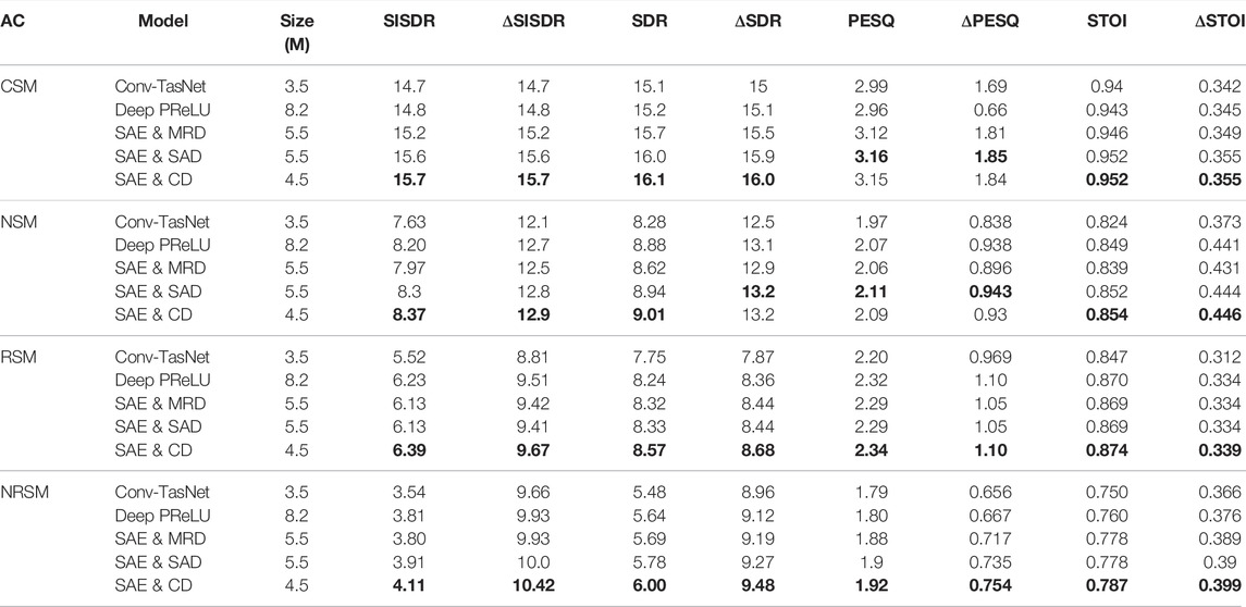
TABLE 6. Comparison of MHA and encoder and decoder against the deep convolutional encoder/decoder Cont-TasNet model proposed by Kadıoğlu et al. (2020). Bold indicates the best performing model for each acoustic condition and metric.
5 Conclusion and Future Work
In this paper novel MHA encoder and decoder networks were proposed for improving TasNet models. The proposed self-attention based MHA encoder demonstrated significant improvement over other encoder baselines across SISDR, SDR, PESQ, and STOI metrics. Three MHA decoders, two using encoder-decoder attention approaches and one using a self-attention approach, were proposed. Performance compared to the original Conv-TasNet model (Luo and Mesgarani, 2019) and a Deep PReLU decoder (Kadıoğlu et al., 2020) baselines varied. The Deep PReLU decoder typically performing better under most acoustic conditions than the encoder-decoder based decoders. The self-attention decoder consistenly performed better than all the other proposed and baseline decoders. Using the MHA encoder alone yielded better performance than any changes to the decoder even with both an MHA encoder and MHA decoder. Further analysis of the intermediate MHA features in the self-attention encoder showed evidence that the network was being more selective in the features being attended to and that many of the channels in the encoder might be mostly redundant.
There are a number of avenues for further research with the proposed MHA encoder and decoders. The MHA encoder demonstrated reliable performance improvements without the significant increase in model size seen in other encoder and decoder networks proposed for Conv-TasNet (Kadıoğlu et al., 2020). One drawback in any implementation using the MHA layer proposed by Vaswani et al. (2017) is the significant memory usage and computational complexity of these network layers. Recent work by Katharopoulos et al. (2020) proposed linear attention layers. Linear attention reduces the quadratic sequential complexity
Data Availability Statement
Publicly available datasets were analyzed in this study. This data can be found here: https://wham.whisper.ai/.
Author Contributions
WR was the main author, proposed using MHA layers in the encoders and decoders, and was involved in devising and implementing the channel sorting algorithm. WR also implemented all the experiments in Section 4. SG contributed to paper writing, assisted with the model analysis sections and provided supervisory support. TH proposed the channel sorting algorithm, had editorial input on this work and provided supervisory support.
Funding
This work was supported by the Centre for Doctoral Training in Speech and Language Technologies (SLT) and their Applications funded by United Kingdom Research and Innovation (grant number EP/S023062/1). This study received funding from 3 M Health Information Systems, Inc. The funder was not involved in the study design, collection, analysis, interpretation of data, the writing of this article or the decision to submit it for publication.
Conflict of Interest
The authors declare that the research was conducted in the absence of any commercial or financial relationships that could be construed as a potential conflict of interest.
Publisher’s Note
All claims expressed in this article are solely those of the authors and do not necessarily represent those of their affiliated organizations, or those of the publisher, the editors and the reviewers. Any product that may be evaluated in this article, or claim that may be made by its manufacturer, is not guaranteed or endorsed by the publisher.
Footnotes
1Conv-TasNet implementation in SpeechBrain: https://github.com/speechbrain/speechbrain/blob/develop/speechbrain/lobes/models/conv_tasnet.py.
References
Bahdanau, D., Cho, K., and Bengio, Y. (2015). “Neural Machine Translation by Jointly Learning to Align and Translate,” in Proc. 3rd International Conference on Learning Representations, ICLR 2015, San Diego, CA, USA. eds. Y. Bengio, and Y. LeCun. doi:10.48550/ARXIV.1409.0473
Benesty, J. (2000). An Introduction to Blind Source Separation of Speech Signals. USA: Kluwer Academic Publishers, 321–329.
Cauchi, B., Gerkmann, T., Doclo, S., Naylor, P., and Goetze, S. (2016). “Spectrally and Spatially Informed Noise Suppression Using Beamforming and Convolutive NMF,” in Proc. AES 60th Conference on Dereverberation and Reverberation of Audio, Music, and Speech (Leuven, Belgium).
Cauchi, B., Kodrasi, I., Rehr, R., Gerlach, S., Jukić, A., Gerkmann, T., et al. (2015). Combination of MVDR Beamforming and Single-Channel Spectral Processing for Enhancing Noisy and Reverberant Speech. EURASIP J. Adv. Signal Process. 2015, 61. doi:10.1186/s13634-015-0242-x
Chen, J., Mao, Q., and Liu, D. (2020). Dual-Path Transformer Network: Direct Context-Aware Modeling for End-To-End Monaural Speech Separation. Interspeech., 2642–2646. doi:10.21437/Interspeech.2020-2205
[Dataset] Cosentino, J., Pariente, M., Cornell, S., Deleforge, A., and Vincent, E. (2020). Librimix: An Open-Source Dataset for Generalizable Speech Separation.
Deng, C., Zhang, Y., Ma, S., Sha, Y., Song, H., and Li, X. (2020). Conv-TasSAN: Separative Adversarial Network Based on Conv-TasNet. Proc. Interspeech, 2647–2651. doi:10.21437/Interspeech.2020-2371
Ditter, D., and Gerkmann, T. (2020). “A Multi-phase Gammatone Filterbank for Speech Separation via TasNet,” in ICASSP 2020 - 2020 IEEE International Conference on Acoustics, Speech and Signal Processing (ICASSP), 36–40. doi:10.1109/icassp40776.2020.9053602
Haeb-Umbach, R., Heymann, J., Drude, L., Watanabe, S., Delcroix, M., and Nakatani, T. (2021). Far-field Automatic Speech Recognition. Proc. IEEE 109, 124–148. doi:10.1109/JPROC.2020.3018668
Hershey, J. R., Chen, Z., Le Roux, J., and Watanabe, S. (2016). “Deep Clustering: Discriminative Embeddings for Segmentation and Separation,” in 2016 IEEE International Conference on Acoustics, Speech and Signal Processing (ICASSP), 31–35. doi:10.1109/ICASSP.2016.7471631
Isik, Y., Roux, J. L., Chen, Z., Watanabe, S., and Hershey, J. R. (2016). “Single-channel Multi-Speaker Separation Using Deep Clustering,” in Proc. 2016 IEEE International Conference on Acoustics, Speech and Signal Processing (ICASSP), 545–549. doi:10.21437/Interspeech.2016-1176
Kadıoğlu, B., Horgan, M., Liu, X., Pons, J., Darcy, D., and Kumar, V. (2020). “An Empirical Study of Conv-TasNet,” in ICASSP 2020 - 2020 IEEE International Conference on Acoustics, Speech and Signal Processing (ICASSP), 7264–7268. doi:10.1109/ICASSP40776.2020.9054721
Katharopoulos, A., Vyas, A., Pappas, N., and Fleuret, F. (2020). “Transformers Are RNNs: Fast Autoregressive Transformers with Linear Attention,” in Proceedings of the 37th International Conference on Machine Learning. Editors H. D. III,, and A. Singh, 5156–5165. doi:10.48550/ARXIV.2006.16236
Kolbaek, M., Yu, D., Tan, Z.-H., Jensen, J., Kolbaek, M., Yu, D., et al. (2017). Multitalker Speech Separation with Utterance-Level Permutation Invariant Training of Deep Recurrent Neural Networks. IEEE/ACM Trans. Audio Speech Lang. Process. 25, 1901–1913. doi:10.1109/TASLP.2017.2726762
Le Roux, J., Hershey, J. R., and Weninger, F. (2015). “Deep NMF for Speech Separation,” in 2015 IEEE International Conference on Acoustics, Speech and Signal Processing (ICASSP), 66–70. doi:10.1109/ICASSP.2015.7177933
Lea, C., Vidal, R., Reiter, A., and Hager, G. D. (2016). “Temporal Convolutional Networks: A Unified Approach to Action Segmentation,” in Computer Vision – ECCV 2016 Workshops. Editors G. Hua,, and H. Jégou (Cham: Springer International Publishing), 47–54. doi:10.1007/978-3-319-49409-8_7
Li, C., Shi, J., Zhang, W., Subramanian, A. S., Chang, X., Kamo, N., et al. (2021). “ESPnet-SE: End-To-End Speech Enhancement and Separation Toolkit Designed for ASR Integration,” in 2021 IEEE Spoken Language Technology Workshop (SLT), 785–792. doi:10.1109/SLT48900.2021.9383615
Lin, Z., Feng, M., Dos Santos, C., Yu, M., Xiang, B., Zhou, B., et al. (2017). “A Structured Self-Attentive Sentence Embedding,” in 2017 Proceedings of the International Conference on Learning Representations (ICLR 2017). doi:10.48550/ARXIV.1703.03130
Luo, Y., Chen, Z., Hershey, J. R., Le Roux, J., and Mesgarani, N. (2017). “Deep Clustering and Conventional Networks for Music Separation: Stronger Together,” in 2017 IEEE International Conference on Acoustics, Speech and Signal Processing (ICASSP), 61–65. doi:10.1109/ICASSP.2017.7952118
Luo, Y., Chen, Z., and Yoshioka, T. (2020). “Dual-path RNN: Efficient Long Sequence Modeling for Time-Domain Single-Channel Speech Separation,” in Proc. 2020 ICASSP, IEEE International Conference on Acoustics, Speech and Signal Processing, 46–50. doi:10.1109/ICASSP40776.2020.9054266
Luo, Y., and Mesgarani, N. (2019). Conv-TasNet: Surpassing Ideal Time-Frequency Magnitude Masking for Speech Separation. IEEE/ACM Trans. Audio Speech Lang. Process. 27, 1256–1266. doi:10.1109/TASLP.2019.2915167
Luo, Y., and Mesgarani, N. (2018). “Tasnet: Time-Domain Audio Separation Network for Real-Time, Single-Channel Speech Separation,” in Proc. 2018 ICASSP, IEEE International Conference on Acoustics, Speech and Signal Processing, 696–700. doi:10.1109/ICASSP.2018.8462116
Maciejewski, M., Wichern, G., McQuinn, E., and Roux, J. L. (2020). “Whamr!: Noisy and Reverberant Single-Channel Speech Separation,” in ICASSP 2020 - 2020 IEEE International Conference on Acoustics, Speech and Signal Processing (ICASSP), 696–700. doi:10.1109/ICASSP40776.2020.9053327
Moritz, N., Adiloğlu, K., Anemüller, J., Goetze, S., and Kollmeier, B. (2017). Multi-channel Speech Enhancement and Amplitude Modulation Analysis for Noise Robust Automatic Speech Recognition. Comput. Speech & Lang. 46, 558–573. doi:10.1016/j.csl.2016.11.004
Ochiai, T., Delcroix, M., Ikeshita, R., Kinoshita, K., Nakatani, T., and Araki, S. (2020). “Beam-TasNet: Time-Domain Audio Separation Network Meets Frequency-Domain Beamformer,” in ICASSP 2020 - 2020 IEEE International Conference on Acoustics, Speech and Signal Processing (ICASSP), 6384–6388. doi:10.1109/ICASSP40776.2020.9053575
Pariente, M., Cornell, S., Deleforge, A., and Vincent, E. (2020). “Filterbank Design for End-To-End Speech Separation,” in ICASSP 2020 - 2020 IEEE International Conference on Acoustics, Speech and Signal Processing (ICASSP), 6364–6368. doi:10.1109/ICASSP40776.2020.9053038
Parsons, T. W. (1976). Separation of Speech from Interfering Speech by Means of Harmonic Selection. J. Acoust. Soc. Am. 60, 911–918. doi:10.1121/1.381172
[Dataset] Ravanelli, M., Parcollet, T., Plantinga, P., Rouhe, A., Cornell, S., Lugosch, L., et al. (2021). SpeechBrain: A General-Purpose Speech Toolkit. doi:10.48550/ARXIV.2106.04624ArXiv:2106.04624
Reddy, C. K. A., Dubey, H., Koishida, K., Nair, A., Gopal, V., Cutler, R., et al. (2021). “INTERSPEECH 2021 Deep Noise Suppression Challenge,” in Proc. Interspeech 2021 (Brno, Czech Republic), 2796–2800. doi:10.21437/Interspeech.2021-1609
Rix, A. W., Beerends, J. G., Hollier, M. P., and Hekstra, A. P. (2001). “Perceptual Evaluation of Speech Quality (Pesq)-a New Method for Speech Quality Assessment of Telephone Networks and Codecs,” in 2001 IEEE International Conference on Acoustics, Speech, and Signal Processing. Proceedings (Cat. No.01CH37221), 749–752. doi:10.1109/ICASSP.2001.941023
Roux, J. L., Wisdom, S., Erdogan, H., and Hershey, J. R. (2019). “SDR - Half-Baked or Well Done?” in Proc. 2019 IEEE International Conference on Acoustics, Speech and Signal Processing (ICASSP), 626–630. doi:10.1109/ICASSP.2019.8683855
Scheibler, R., Bezzam, E., and Dokmanic, I. (2018). “Pyroomacoustics: A python Package for Audio Room Simulation and Array Processing Algorithms,” in Proc. 2018 IEEE International Conference on Acoustics, Speech and Signal Processing (ICASSP), 351–355. doi:10.1109/ICASSP.2018.8461310
Schmidt, M. N., and Olsson, R. K. (2006). “Single-channel Speech Separation Using Sparse Non-negative Matrix Factorization,” in Proc. Interspeech 2006. doi:10.21437/Interspeech.2006-655
Shi, Y., and Hain, T. (2021). “Supervised Speaker Embedding De-mixing in Two-Speaker Environment,” in 2021 IEEE Spoken Language Technology Workshop (SLT 2021). doi:10.1109/SLT48900.2021.9383580
Shi, Z., Lin, H., Liu, L., Liu, R., Han, J., and Shi, A. (2019). Deep Attention Gated Dilated Temporal Convolutional Networks with Intra-parallel Convolutional Modules for End-To-End Monaural Speech Separation. Proc. Interspeech, 3183–3187. doi:10.21437/Interspeech.2019-1373
Stoller, D., Ewert, S., and Dixon, S. (2018). “Wave-U-Net: A Multi-Scale Neural Network for End-To-End Audio Source Separation,” in Proceedings of the 19th International Society for Music Information Retrieval Conference, ISMIR, 334–340. doi:10.48550/ARXIV.1806.03185
Subakan, C., Ravanelli, M., Cornell, S., Bronzi, M., and Zhong, J. (2021). “Attention Is All You Need in Speech Separation,” in Proc. 2021 IEEE International Conference on Acoustics, Speech and Signal Processing (ICASSP), 21–25. doi:10.1109/ICASSP39728.2021.9413901
Taal, C. H., Hendriks, R. C., Heusdens, R., and Jensen, J. (2010). “A Short-Time Objective Intelligibility Measure for Time-Frequency Weighted Noisy Speech,” in 2010 IEEE International Conference on Acoustics, Speech and Signal Processing, 4214–4217. doi:10.1109/ICASSP.2010.5495701
Vaswani, A., Shazeer, N., Parmar, N., Uszkoreit, J., Jones, L., Gomez, A. N., et al. (2017). “Attention Is All You Need,” in Proceedings of the 31st International Conference on Neural Information Processing Systems (Red Hook, NY, USA: Curran Associates Inc), 6000–6010. doi:10.5555/3295222.3295349
Wang, D., and Chen, J. (2018). Supervised Speech Separation Based on Deep Learning: An Overview. IEEE/ACM Trans. Audio Speech Lang. Process. 26, 1702–1726. doi:10.1109/TASLP.2018.2842159
Watanabe, S., Hori, T., Karita, S., Hayashi, T., Nishitoba, J., Unno, Y., et al. (2018). ESPnet: End-To-End Speech Processing Toolkit. Proc. Interspeech, 2207–2211. doi:10.21437/Interspeech.2018-1456
Wichern, G., Antognini, J., Flynn, M., Zhu, L. R., McQuinn, E., Crow, D., et al. (2019). WHAM!: Extending Speech Separation to Noisy Environments. Proc. Interspeech, 1368–1372. doi:10.21437/Interspeech.2019-2821
Yang, G.-P., Tuan, C.-I., Lee, H.-Y., and Lee, L.-s. (2019). Improved Speech Separation with Time-And-Frequency Cross-Domain Joint Embedding and Clustering. Proc. Interspeech, 1363–1367. doi:10.21437/Interspeech.2019-2181
Keywords: tasnet, speech separation, speech enhancement, encoder, decoder, attention
Citation: Ravenscroft W, Goetze S and Hain T (2022) Att-TasNet: Attending to Encodings in Time-Domain Audio Speech Separation of Noisy, Reverberant Speech Mixtures. Front. Sig. Proc. 2:856968. doi: 10.3389/frsip.2022.856968
Received: 17 January 2022; Accepted: 13 April 2022;
Published: 11 May 2022.
Edited by:
Nobutaka Ito, University of Tokyo, JapanReviewed by:
Yoshiki Masuyama, Tokyo Metropolitan University, JapanTimo Gerkmann, University of Hamburg, Germany
Copyright © 2022 Ravenscroft, Goetze and Hain. This is an open-access article distributed under the terms of the Creative Commons Attribution License (CC BY). The use, distribution or reproduction in other forums is permitted, provided the original author(s) and the copyright owner(s) are credited and that the original publication in this journal is cited, in accordance with accepted academic practice. No use, distribution or reproduction is permitted which does not comply with these terms.
*Correspondence: William Ravenscroft, andyYXZlbnNjcm9mdDFAc2hlZmZpZWxkLmFjLnVr