 Ana Oprisan
 Sorinel Adrian Oprisan
- Department of Physics and Astronomy, College of Charleston, Charleston, SC, United States
Introduction: The gray-level co-occurrence matrix (GLCM) reduces the dimension of an image to a square matrix determined by the number of gray-level intensities present in that image. Since GLCM only measures the co-occurrence frequency of pairs of gray levels at a given distance from each other, it also stores information regarding the gradients of gray-level intensities in the original image.
Methods: The GLCM is a second-order statical method of encoding image information and dimensionality reduction. Image features are scalars that reduce GLCM dimensionality and allow fast texture classification. We used Haralick features to extract information regarding image gradients based on the GLCM.
Results: We demonstrate that a gradient of k gray levels per pixel in an image generates GLCM entries on the kth parallel line to the main diagonal. We find that, for synthetic sinusoidal periodic gradients with different wavelengths, the number of gray levels due to intensity quantization follows a power law that also transpires in some Haralick features. We estimate bounds for four of the most often used Haralick features: energy, contrast, correlation, and entropy. We find good agreement between our analytically predicted values of Haralick features and the numerical results from synthetic images of sinusoidal periodic gradients.
Discussion: This study opens the possibility of deriving bounds for Haralick features for targeted textures and provides a better selection mechanism for optimal features in texture analysis applications.
1 Introduction
Image processing can be performed in dual spaces, such as the Fourier transform or image space. Direct imaging allows the fastest possible information retrieval for image classification. Among the many properties of an image, texture is the most often used for classification. “Texture is an innate property of virtually all surfaces, the grain of wood, the weave of a fabric, the pattern of crops in a field, etc. […] Texture can be evaluated as being fine, coarse, or smooth; rippled, moiled, irregular, or lineated” (Haralick et al., 1973). The critical assumption in texture analysis and classification based on the gray-level co-occurrence matrix (GLCM) introduced by Haralick is that “…texture information in an image I is contained in the overall or ‘average’ spatial relationship which the gray tones in the image have to one another” (Haralick et al., 1973).
The initial applications of Haralick features used photomicrographs of sandstone and aerial photographs and satellite images to classify types of stone and determine land-use categories (Haralick et al., 1973; Haralick, 1979). From the beginning, Haralick’s features were also applied in medical imaging to enable personalized medicine by taking advantage of clinical imaging data. The first automatic screening texture-based analysis for identifying and classifying pneumoconiosis was developed by Hall et al. (1975). Although they did not use Haralick features for classification, they established that only invariant measures of pixel relationships should be used for medical diagnosis. Haralick et al. (1973) and Haralick (1979) also noted that the most valuable features for texture classifications are the angular second moment, entropy, sum entropy, difference entropy, information measure of correlation, and the maximal correlation features that are due to gray-level quantization invariance. Recent advances in machine learning and AI have led to novel approaches in X-ray radiodiagnosis which are primarily focused on optimized versions of convolutional neural networks (CNNs) (Akhter et al., 2023). The first automatic system based on Haralick features used digitized lung X-rays and identified black lung disease with 96% accuracy (Kruger et al., 1974; Abe et al., 2014), while physician accuracy varies from 86% to 100% (Hall et al., 1975). Although the nomenclature was not yet standardized at the time of the first large-scale pneumoconiosis study (Kruger et al., 1974) using Haralick features (Haralick et al., 1973; Haralick, 1979), the five features used for patient classification were “autocorrelation” (similar to the normalized correlation feature f3 from Eq. 10), the “moment of inertia” (similar to the contrast feature f2 from Eq. 9), a similarity feature (similar to inverse difference momentum f5 from Eq. 12), a conditional entropy (similar to the entropy feature f9 from Eq. 16), and “another dissimilarity measure” (similar to the contrast feature except using absolute value instead of the square distance between gray levels in GLCM). The volume of radiation oncology on radiographic images for diagnosis and treatment is increasing exponentially. It requires new fast direct imaging analysis, such as segmentation and texture analysis based on Haralick features (Bodalal et al., 2019). All medical imaging modalities (CT, MRI, PET, and ultrasound) display the image as grayscale, and the image features (as many as a couple of thousand) are extracted for classification in machine learning-assisted image processing (Devnath et al., 2022; Wang et al., 2022; Ferro et al., 2023a). Radiomic texture features were applied to images to classify pulmonary nodules as benign or malignant, with a correct classification rate of 90.6% in 1999 (McNitt-Gray et al., 1999). McNitt-Gray et al. (1999) first identified the most relevant Haralick features in pulmonary nodule classification. They found that a reasonable (over 90%) classification accuracy can be obtained with only three features: contrast, sum entropy, and difference variance. Their study also highlighted that the selection of displacement vectors is critical for classification accuracy. Non-oncological classification tasks in the kidneys alone have included differentiation between benign and malignant lesions and lipid-poor angiomyolipomas from renal cell carcinoma (RCC) (Raman et al., 2014; Yan et al., 2015; Jeong et al., 2019; Ferro et al., 2023b; Criss et al., 2023). Classification tasks have also successfully classified lesions in the liver, pancreas, and bowel (Song et al., 2014; Raman et al., 2015; Permuth et al., 2016; Jeong et al., 2019; Cao et al., 2022). The texture features outperformed standard uptake value (SUV) parameters in PET scan images, including mean SUV, maximum SUV, peak SUV, metabolic tumor volume, and total lesion glycolysis (Cook et al., 2013; Feng et al., 2022). Texture features are helpful for image contouring, tissue identification, classification tasks, disease staging, treatment response prediction, disease-free survival, overall survival estimation, risk stratification, response classification, and real-time response monitoring. Among the most used features in medical imaging are first-order statistical descriptors (mean, range, and standard deviation), shape descriptors, and texture features (El-Baz et al., 2011). In addition to direct imaging-based features such as Haralick’s, there are also wavelet-based feature filter banks (Mallat, 1989; Soufi et al., 2018; Prinzi et al., 2023).
In addition to biomedical imaging, Haralick features have been applied to detecting intrusion to mitigate cybersecurity attacks (Azami et al., 2019; Baldini et al., 2021). Intrusion detection algorithms identify unauthorized intruders and attacks on various electronic devices and systems such as computers, network infrastructures, and ad hoc networks (Lunt, 1993; Baldini et al., 2017).
Crowd abnormality detection, such as for flash mobs, is a public safety concern, and real-time identification and intervention are crucial for reducing casualties (Sivarajasingam et al., 2003; Lloyd et al., 2017). The difficulty of crowd abnormality detection is the great amount of data feeds available. By some estimates, there is one surveillance camera per 35 people in the United Kingdom (Serrano Gracia et al., 2015) combined with a very low human accuracy of 19% for detecting abnormalities while simultaneously observing four video feeds (Voorthuijsen et al., 2005). The default video tracking algorithm is based on the optical flow method (Kratz and Nishino, 2012), which has significant drawbacks when applied to crowds (Wang and Xu, 2016). A considerable data dimensionality reduction was obtained using GLCM (Ryan et al., 2011), which allowed the fast detection of abnormalities (Lloyd et al., 2017).
1.1 Gray-level co-occurrence matrix (GLCM)
Throughout this study, the pixel coordinate definition originates at the top-left corner of an image with the x-direction horizontal to the right and a y-direction vertically downward (Figure 1A). As a result, the matrix representation of an image has its first (line) index associated with the y-direction and the second (column) index with the x-direction, that is, I (line index, column index) = I (y, x) (Figure 1B). An image I (y, x) of size Ny × Nx gives the intensity at location (pixel) of coordinates (y, x) by discrete numbers from
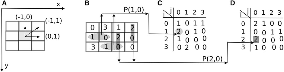
FIGURE 1. GLCM displacement vector and marginal probabilities. (A) By convention, the x-direction runs horizontally to the right, and the y-direction is vertically downward, with the image’s origin at the upper-left corner. The pixel of interest in the grayscale image I (y, x) has the nearest horizontal neighbor to the right described by the offset, or displacement, vector d =(Δy =0, Δx =1) and the nearest vertically upward neighbor given by d =(Δy =−1, Δx =0). (B) A two-bit image is scanned for all horizontal nearest neighbors to the right of the reference pixel with a displacement vector d =(Δy =0, Δx =1). The two elliptical shaded areas show two pairs with gray-level intensities i =1, j =0, i.e., P(1,0)=2. GLCM is shown in panel (C). The two rectangular shaded areas in panel (B) show vertically upward neighbors with a displacement vector d =(Δy =−1, Δx =0). The two pairs with i =2, j =0, i.e., P(2,0)=2, are shown in panel (D).
The gray level co-occurrence matrix (GLCM) counts the number of occurrences of the reference gray level i at a distance specified by the horizontal and vertical increments d = (Δy, Δx) from the gray level j (Haralick et al., 1973):
where # denotes the number of elements in the set, the coordinates of the reference gray level i are (yi, xi), and the coordinates of the neighbor pixel with gray level j are (yj = yi + Δy, xj = xi + Δx). In GLCM, the first index is the reference or starting point of the displacement vector d. For example, an offset d = (Δy = 0, Δx = 1) means that the row index (y-direction) does not change because Δy = 0 and the column index increases (x-direction) by one unit (Δx = 1), that is, the new location is the horizontal nearest neighbor to the right of the reference pixel, as shown by the shaded ellipses for i = 1, j = 0 in Figure 1B. The corresponding GLCM for d = (0, 1) is shown in Figure 1C. Similarly, an offset d = (Δy = −1, Δx = 0) means that the row index (y-direction) decreases by one unit (vector pointing vertically upward), and the column index is constant. The pairs are upward vertical nearest neighbors, as shown by the shaded rectangles in Figure 1B and the corresponding GLCM in Figure 1D. In their seminal paper on GLCM features, Haralick et al. (1973) focused on the eight nearest neighbors of the reference pixel in Figure 1 and used the magnitude |d| of the displacement vector d = (Δy, Δx) and the corresponding angle θ = tan−1 (Δy/Δx) to the nearest neighbor.
Although it is common practice in GLCM evaluation to consider toroidal periodic boundary conditions, we did not use them in this study. In the original definition of GLCM given by Haralick et al. (1973), there is a symmetry that allows both 1,2 and 2,1 pairings to be counted as the number of times the value 1 is adjacent to the value 2. Here, we used a stricter approach to define the occurrence matrix that does not double count such occurrences; consequently, our GLCMs are not always symmetric.
GLCM belongs to the class of second-order statistical methods for image analysis and is based on the joint probability distribution of gray-level intensities at two image pixels. The first-order statistic is based on the image histogram and the statistical values, such as mean image intensity, standard deviation, and skewness. The justification of the GLCM method is based on experiments on the human visual system that showed that “…no texture pair can be discriminated if they agree in their second-order statistics” (Julesz, 1975).
The number of possible pairs in the image often normalizes GLCM. For example, in an Nx × Ny image, there are Rx = (Nx − 1)Ny horizontal pairs and Ry = (Ny − 1)Nx vertical pairs with a displacement vector d of one unit. In the example shown in Figure 1, since the image is 3 × 4 pixels, the GLCM normalization factors are Rx = 9 and Ry = 8. The corresponding normalized GLCM values in Figure 1C are, for example, p(1, 0) = P(1, 0)/Rx = 2/9 and for Figure 1D are p(2, 0) = P(2, 0)/Ry = 2/8. In the following, un-normalized GLCM is labeled with capital letters such as P(i, j), whereas its normalized version is labeled p(i, j). The advantage of the normalized GLCM is that, regardless of the size of the image or the number of gray levels,
Haralick features have received much recent attention due to the advance of machine learning and artificial intelligence algorithms capable of accurately and quickly classifying textures over a wide range of applications, such as biomedical imaging (Cao et al., 2022; Devnath et al., 2022; Feng et al., 2022; Wang et al., 2022; Ferro et al., 2023a; Akhter et al., 2023; Ferro et al., 2023b; Criss et al., 2023; Nakata and Siina, 2023; Prinzi et al., 2023), cybersecurity (Lunt, 1993; Chang et al., 2019; Karanja et al., 2020; Baldini et al., 2021), or crowd abnormality (Sivarajasingam et al., 2003; Lloyd et al., 2017; Naik and Gopalakrishna, 2017). However, beyond five-decade-old definitions (Haralick et al., 1973), little progress has been made on the theoretical and analytical understanding of Haralick features, deriving theoretical lower and upper bounds, the dependence of GLCM and Haralick features on image depth, and other related issues. We started this study by observing that Haralick features are measures of light intensity gradients in images. To derive bounds for Haralick features, we determined the symmetries of GLCM induced by the linear gradients present in images. Such symmetries allowed us to estimate the marginal probabilities (Section 2) necessary for analytically estimating Haralick feature bounds. We then generated synthetic gradients, such as vertical stripes of different gray-level intensities, and compared our theoretical predictions against numerical calculations of Haralick features. While we used all 14 Haralick features (Section 2), only four are relevant to the synthetic patterns we investigated (Section 3). We also showed that some features, like contrast and homogeneity, are redundant for the synthetic images generated.
2 Methods: Haralick GLCM features
The un-normalized GLCM P(i, j) gives the number of occurrences of gray level j at a distance Δx and Δy from the current location of the reference pixel with gray level i in an image. Assuming that there are
with the obvious property that
2.1 Marginal probability distributions
The x-direction marginal probability distribution, or marginal row probability, can be obtained by summing the rows of GLCM p(i, j):
as shown in Figure 2A. For example, px(0) is the sum of all row elements with intensity i = 0 at the reference point, or the starting point of displacement vector d in Figure 1A regardless the intensity of its endpoint neighbors. Similarly, the mean and variance of GLCM along px(i) are as follows:
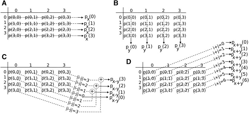
FIGURE 2. Marginal probability distributions from GLCM. (A) The probability of finding a gray-level intensity i along the horizontal x-direction in the image is px(i) and along the y-direction is py(i) [see panel (B)]. (C) The probability of finding a contrast of k gray levels in the image is px−y(k) and is determined by the elements parallel to the primary diagonal of GLCM. (D) The probability of finding an intensity sum of the k gray level in the image is px+y(k) and is determined by the elements parallel to the secondary diagonal of GLCM.
The y-direction marginal probability distribution, or marginal column probability, can be obtained by summing the columns of GLCM p(i, j)
as shown in Figure 2B. For example, py(0) is the sum of all column elements with an endpoint intensity i = 0 (Figure 1A) regardless the intensity of the reference (starting) point.
The marginal distribution of a given contrast k = |i − j| between the reference pixel intensity i and endpoint neighbor intensity j is as follows:
where δm,n is Kronecker’s delta symbol. For example, px−y(0) is the sum of all GLCM entries along the primary diagonal because these elements have no contrast between the reference i and the endpoint j of the vector d (Figure 2C). Similarly, the sum of GLCM entries along the first-order diagonal parallel to the primary diagonal has a contrast of k = j − i = 1 between the reference i and the endpoint j of GLCM and determines the element px−y(1) of the marginal distribution px−y.
The marginal distribution of a given sum of gray-level intensity k = i + j between the reference pixel intensity i and the endpoint neighbor intensity j is
and can be visualized as corresponding sums along the secondary diagonals (Figure 2D).
2.2 Haralick texture features
While there is no standard notation for Haralick features, we will follow the original (Haralick et al., 1973; Haralick, 1979).
1) Angular second momentum (ASM) or energy is a measure of the homogeneity of the image and is defined as
When pixels are very similar, the ASM value will be large. For a quantization scheme with
2) Contrast (CON) measures local variations present in the image and is defined as
When i and j are equal, there is no contrast k = j − i between pixels; therefore, px−y(k) has weight k = 0 in f2 along the primary diagonal of GLCM. If k = |i − j| = 1, there is a small contrast between neighbor pixels, and px−y(k) contributes a weight of 1 to f2. The weight of px−y(k) increases quadratically as the contrast k = |i − j| increases. For example, if only the primary diagonal elements of the GLCM are populated, then the contrast is minimum f2 = 0. This feature measures the variation between neighboring pixels (larger differences get square law weights). It can also be viewed as a measure of the spread of values in the GLCM matrix. Contrast is associated with the average gray level difference between neighboring pixels and is similar to variance. However, contrast is preferred due to reduced computational load and its effectiveness as a spatial frequency measure. Energy and contrast are the most significant parameters for visual assessment and computational load to discriminate between textural patterns.
3) Correlation (COR) is a measure of the linear dependency of gray levels of neighboring pixels and is defined as
COR describes how a reference pixel is related to its neighbor: 0 is uncorrelated and 1 is perfectly correlated. This measure is similar to the familiar Pearson correlation coefficient.
4) Variance (VAR)
Variance is a measure of the dispersion of the values around the mean of combinations of reference and neighbor pixels. This feature assigns increasing weight to greater gray-value differences. The mean value μ was not defined in Haralick’s original studies and is given by
This statistic measures heterogeneity and correlates with first-order statistical variables such as standard deviation. Variance increases when the gray-level values differ from their mean.
5) Inverse difference momentum (IDM) or homogeneity measures the local homogeneity and has a high value when the local gray level is uniform. Its definition is as follows:
IDM measures the closeness of the distribution of the GLCM elements to the GLCM diagonal. The IDM weight value is the inverse of the contrast weight, with weights decreasing quadratically away from the diagonal. Sometimes, a new homogeneity measure is used:
6) Sum Average (SA)
Sum average measures the sum of the average of all gray levels.
7) Sum variance (SV)
Sum variance is a measure of heterogeneity that places higher weights on neighboring intensity level pairs that deviate more from the mean. The uniform (flat) distribution of the sum of gray levels has maximum entropy.
8) Sum entropy (SE)
Sum entropy is a measure of non-uniformity in the image or the complexity of the texture.
9) Entropy
Entropy takes on its maximum value when a probability distribution is uniform (completely random texture), and its minimum value is 0 when it becomes deterministic (all grayscale values in the image are identical). If the entropy f9 is defined using the base-2 logarithm log2 (), then f9 is measured in bits. Entropy measures the disorder of an image and achieves its greatest value when all elements in the GLCM matrix are equal. The entropy measure is also called the “Shannon diversity”. It is high when the pixel values of GLCM have varying values. Entropy is inversely proportional to the angular second moment; this statistic measures the disorder or complexity of an image. Entropy is large when the image is not texturally uniform—many GLCM elements have very small values. Complex textures tend to have high entropy: entropy is strongly but inversely correlated with energy.
10) Difference variance (DV)
where the difference average (DA) is given by
11) Difference entropy (DE)
Difference entropy measures the randomness or lack of structure or order in the image contrast. The uniform (flat) distribution of the difference of gray levels has maximum entropy.
12) Information Measures of Correlation Feature 1
where
13) Information Measures of Correlation Feature 2
where
14) Maximal correlation coefficient
where
3 Results
GLCM and Haralick features are challenging to interpret as they have second-order statistical correlation characteristics among pixels. Here, we provide a detailed analytical and computational analysis of synthetic images to gain insights into the GLCM’s meaning. Since Haralick features are based on pairwise distribution along different directions in the image, the most fundamental type of texture is a gradient of gray levels (Figures 3A1 or 3A2). Consequently, gradients of different intensities (in gray levels per pixel) will be found along the corresponding lines parallel to the principal (main) diagonal of GLCM. For example, if there is no gradient along a particular direction (uniform gray-level intensity), the respective pixels will contribute only to the main diagonal. A gradient of one gray level per pixel in a given direction will only contribute to the first line parallel to the main diagonal of GLCM (Figure 3C1), as explained in detail in the following.
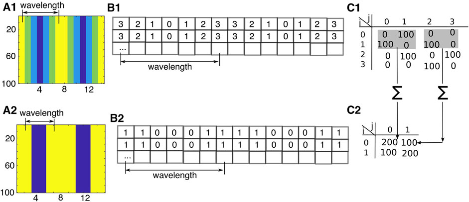
FIGURE 3. Vertical stripes synthetic images. (A1) Vertical stripes of constant intensity with a horizontal gradient of 1 gray level per pixel with a b = 2-bit depth. The images were rendered in color to emphasize the differences between gray-level stripes. Each line is 1 pixel wide. (B1) Gray-level intensities for the vertical stripes in panel (A1). (C1) GLCM for the image in panel (A1). (A2) Reduced 1-bit depth of the original image in panel (A1). (B2) Gray-level intensities for the 1-bit depth image in (A2). (C2) GLCM for the image in panel (A2). GLCM of 1-bit depth is the convolution of non-overlapping 2×2 kernels (shaded areas in panel c1) with GLCM of the 2-bit image.
3.1 From image patterns to GLCM patterns
3.1.1 Horizontal displacement vectors and GLCM entries for constant gradients of gray levels
Although the results are valid for an arbitrary number of gray levels, we could only produce a manageable size GLCM fitting the printed page by using a b = 2-bit gray-level image with the fixed number of lines Ny = 100, similar to the case shown in Figure 1. The most straightforward synthetic images are composed of vertical lines with a horizontal gradient of gray-level intensities: first vertical line of intensity 2b − 1 = 3, the next vertical line of intensity 2, and so on. In this case, the gradient is one gray level per pixel along the horizontal direction with the “natural” displacement vector d = (Δy, Δx) = (0, 1) (Figure 3A1). As the synthetic image in Figure 3A1 is scanned from left to right, we noticed that, first, there is a gray-level transition for 3 to 2, P(3, 2) = 1, followed by P(2, 1) = 1 until we reached the lowest gray level with P(1, 0) = 1 (Figure 3B1). One gray level per pixel gradient allows one-to-one mapping between gray levels
The wavelength, λ of the periodic structure marked in Figure 3A1 is λ = Nx/Mx pixels, which can be determined more generally as the ratio of the image size Nx × Ny divided by the factor that multiplies GLCM. For the 2-bit depth image in Figure 3A1, the actual grayscale values are shown in Figure 3B1. GLCM for the first wavelength λ in Figure 3A1 is shown in Figure 3C1. There are no diagonal elements in GLCM (Figure 3C1), and they can only occur in two different ways. The first possibility is that a vertical stripe, like that shown in Figures 3A1, A2, is more than one pixel wide. For example, in Figure 3A1 and the numerical example shown in Figure 3B1, the line of gray level 3 has a width w3 larger than one pixel and contributes w3 − 1 times to the diagonal element P (3, 3). In this example, the gray level 3 of the first wavelength λ is followed by a vertical strip of the same gray level value from the next wavelength— w3 = 2. Consequently, GLCM for the entire image shown in Figure 3A1 includes P(3, 3) = (w3 − 1)*Ny = 1*100 (Table 1) which accounts for the fact that there is a two-pixel-wide vertical strip of gray level 3 in Figure 3A1.
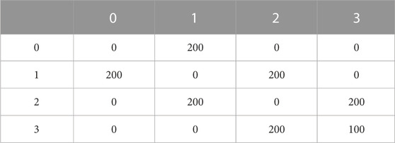
TABLE 1. GLCM for the entire image in Figure 3A1 with a horizontal displacement vector d =(Δy, Δx)=(0,1), i.e., rightward displacement, or d =(0,−1), i.e., leftward displacement.
3.1.2 Bit depth reduction of images and their effect on GLCM
Bit depth reduction can occur during image compression or other image processing operations that require casting the image intensity to a lower depth. Therefore, the second possibility for generating a non-zero diagonal element in the GLCM is a bit depth reduction (Figure 3A2) where the original image from Figure 3A1 was reduced from 2-bit (four gray levels) to 1-bit (two gray levels) depth. Such a bit depth reduction is generated by dropping the least significant digit in the binary representation of the gray levels. The bit depth reduction is a convolution of the higher depth intensity GLCM with a 2 × 2 non-overlapping kernel, as shown in Figure 3C1 with the shaded rectangles. All occurrences involving gray levels 0 and 1 in the 2-bit depth GLCM, such as P(0, 0), P(0, 1), P(1, 0), and P(1, 1) in the 2-bit GLCM shown in Figure 3C1, collapse to gray level 0 after depth reduction to 1-bit. This convolution is suggested in Figure 3C1 by the symbol Σ along the arrow that maps the 2 × 2 kernel into the new GLCM values shown in Figure 3C2. For clarity, we insert a subscript to GLCM to indicate its bit depth, such that
Similarly, gray levels 2 and 3 in the 2-bit image depth shown in Figure 3A1 collapse to the new gray level 1 in the 1-bit image shown in Figure 3A2.
3.1.3 Vertical displacement vectors and the GLCM entries for constant gradients of gray levels
GLCM of Figure 3A1 along the vertical direction with a displacement vector d = (Δy, Δx) = (−1, 0) or d = (Δy, Δx) = (1, 0) contains only diagonal elements as there is no gray level gradient along the vertical direction (Table 2). For example, there is only one vertical strip of gray level 0 on the first wavelength λ, marked in Figure 3A1, which contains P(0, 0) = (Ny − 1) = 99 gray level pairs of 0 and 0 intensities along the vertical direction (see Table 2).
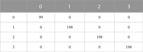
TABLE 2. GLCM for the entire image in Fig. 3a1 with a vertical displacement vector d =(Δy, Δx)=(−1,0), i.e., downward displacement, or d =(1,0), i.e., upward displacement.
Therefore, a zero gradient—no change in gray level—along a given displacement vector leads to non-zero main diagonal elements in GLCM. A gradient of one gray level per pixel leads to non-zero elements along the first upper and lower parallel lines to the main diagonal, as seen in Figure 3C1 and Table 1. Similarly, a gradient of two gray levels per pixel would lead to non-zero GLCM values for P(0, 2), P(1, 3), P(3, 1), and P(2, 0), which are elements along the second upper and lower parallel lines to the main diagonal.
Because GLCM is a lower-dimensional
3.2 From GLCM patterns to Haralick features
Section 3.1 shows the relationship between patterns, such as gray-level gradients, in images and the structure of GLCM. Haralick features (Section 2) represent another level of dimension reductions as the entire
Given that a dimension reduction produces a feature that is even more ambiguous than GLCM, it being impossible to infer the original image patterns, we focus here on the following:
1) Using synthetic 8-bit and 1,024 × 1,024 pixel images with known patterns or textures (Figure 4) and linking them to Haralick features.
2) Investigating the effect of gray-level quantization in Section 3.2.1 (see Eq. 23 and Eq. 24) induced by periodic gradients.
3) Determining the bit depth reduction effect on energy (Section 3.2.2.1), contrast (Section 3.2.3.1), correlation (Section 3.2.4.1), and entropy (Section 3.2.5.1) features.
4) Estimating lower and upper bounds for energy (Section 3.2.2.2), contrast (Section 3.2.3.2), correlation (Section 3.2.4.2), and entropy (Section 3.2.5.2) features for specific gray-level distributions, such as random intensities or uniform gray levels.
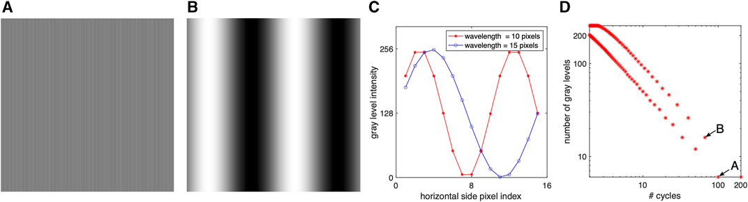
FIGURE 4. Vertical stripe synthetic images of 1,024×1,024 pixels with 8-bit depth. (A) Vertical stripes of wavelength λ =10 pixels. (B) Vertical stripes of wavelength 200 pixels. (C) Different quantization schemes generated by two wavelengths of λ =10 (* symbol), respectively, λ =15 (o symbol), pixels. (D) As wavelength λ decreases and the number of cycles that fit into the Nx =1,024 pixel increases, quantization maps to fewer gray levels.
In the following, we only review some of the most frequently used and relevant Haralick’s features and make theoretical predictions regarding their values in the aforementioned two cases that are amenable to analytic solutions. All our analytical derivations were subsequently checked by numerical simulations using synthetic textures. For all numerical simulations, we generated synthetic images where the gray levels vary sinusoidally along the horizontal direction according to sin (2πx/λ) where x is the pixel index from 1 to Nx = 1,024, as shown in Figures 4A (for λ = 10 pixels) and B (for λ ≈ 200 pixels).
3.2.1 Gray-level quantization of sinusoidal gradients of variable wavelength
While all sine waves cover b = 8-bit depth
with an RMSE value of 1.3326 and an adjusted R2 = 0.9995. For the alternative line that starts at ‘B’,
with an RMSE value of 2.0835 and an adjusted R2 = 0.9990.
3.2.2 Analytical estimates for energy feature
In the following, we provide analytical estimates of how a bit reduction affects GLCM and the corresponding Haralick feature. While some Haralick features are normalized, such as correlation, most are not, and there are no theoretical lower and upper bounds in the literature. We provide systematic derivations of bounds for each of the selected features along (a) vertical displacement vectors, (b) horizontal displacement vectors, and (c) after a random reshuffling of image pixels.
3.2.2.1 Bit-depth reduction affects angular second momentum (ASM) or energy
Based on Eq. 8, the lowest ASM corresponds to a random distribution of gray levels and the maximum to a uniform image. As previously noted, reducing the image’s bit depth by one unit makes every new entry in the lower-depth GLCM the sum of the elements in 2 × 2 sub-arrays from the higher-depth GLCM. Using Eq. 22, one finds
3.2.2.2 Lower and upper bounds for angular second momentum (ASM) or energy
3.2.2.2.1 Vertical displacement vectors
A log–log plot of the ASM, or energy, feature for the original image Figure 5A1 shows that its value is constant across all images for the vertical displacement vectors (green solid circles and blue crosses). This is expected as GLCM for the vertical strips (Table 2) has only diagonal elements with little to no change as we add more vertical stripes. For such homogeneous patterns, such as single pixel-wide vertical stripes measured along the vertical displacement vector, the GLCM diagonal entries are
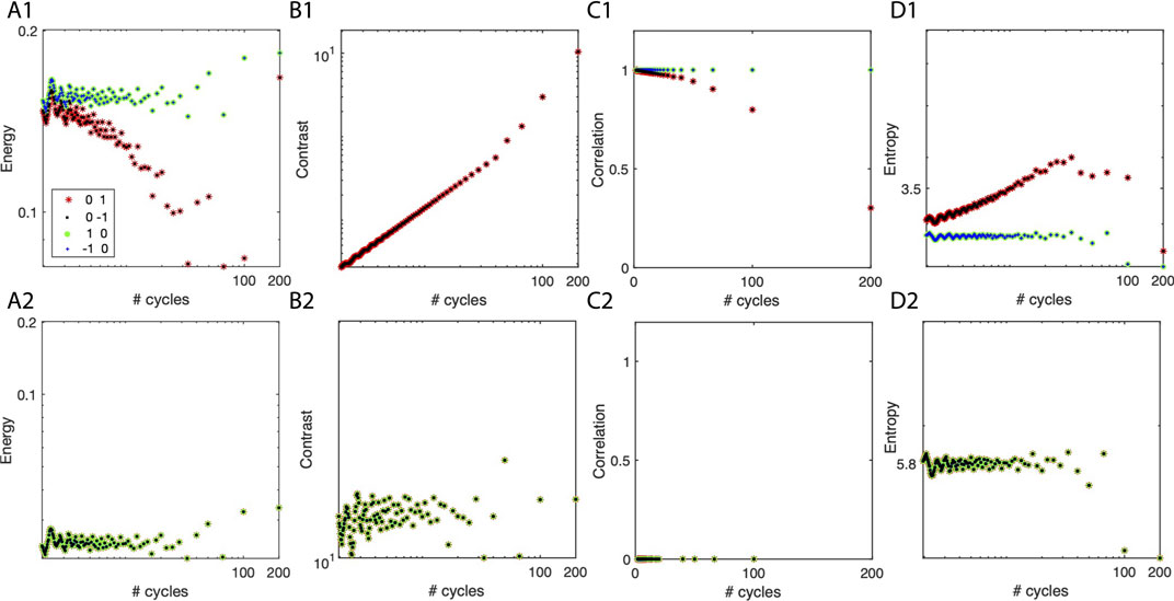
FIGURE 5. Selected Haralick features for vertical stripes of variable wavelength. Top panels (A1–D1) are the Haralick features of the 8-bit images of vertical stripes of variable wavelengths, such as those shown in Figures 4A, B. The bottom panels (A2–D2) are the Haralick features for the same images, with all pixels randomly reshuffled. (A1, A2) Log–log plot of energy for horizontal displacements (red stars and black squares) and vertical displacements (green dots and blue crosses). (B1, B2) Regardless of the direction of the displacement vector, the log–log plot of the contrast feature overlaps. (C1, C2) The correlation feature is the maximum possible for a vertical displacement vector and decreases along the horizontal direction. (D1, D2) The log–log plot of entropy is constant for the vertical displacement vector and increases along the horizontal direction.
3.2.2.2.2 Horizontal displacement vectors
GLCM along the horizontal displacement direction is similar to Table 1, where most occurrences are parallel to the main diagonal. For horizontal displacement vectors and a very short wavelength of λ = 10 pixels, we previously found (Figure 4) that there are only
3.2.2.2.3 Random reshuffling of pixels
The energy of all displacement vectors for randomly reshuffling the pixels in the image is the same and very low, as expected (Section 2). Indeed, for a random distribution of pixel intensities, we expect
To summarize, the lower bound of the angular second momentum (ASM) or energy is
3.2.3 Bound estimates for contrast feature
3.2.3.1 Bit depth reduction effect on contrast
While most Haralick features are based on GLCM p (i, j), the contrast is based on the GLCM subset px−y(k) of elements parallel to that primary diagonal (Eq. 9). If all elements of GLCM are along the primary diagonal at a given bit depth of px−y (0) = 1, then the contrast is f2 = 0 and will be 0 for all subsequent depth-reduced images. The contrast continuously decreases by bit-depth reduction— f2,1bit ≤ f2,2bit. For example, assuming that all elements of 2-bit GLCM are distributed to achieve maximum contrast of 3—px−y,2bit (3) = 1—then the contrast is f2,2bit = 32. A 1-bit depth reduction means that the maximum contrast is 1 and px−y,2bit (1) = 1, which gives f2,1bit = 12.
3.2.3.2 Lower and upper bounds bit for contrast
3.2.3.2.1 Vertical displacement vectors
In such cases, the only elements of the occurrence matrix are along the main diagonal, which means that the contrast in Figure 5A2 is 0 (not shown due to the log–log scale).
3.2.3.2.2 Horizontal displacement vectors
The contrast along the horizontal displacement vector increases with the number of cycles, Mx. This is because a larger number of cycles means that the 8-bit gray levels will fit on a smaller scale, leading to a larger gradient k = |i − j| between gray levels—the GLCM entries will be aligned parallel to the main diagonal, but farther from it. As a result, the contrast increases (Figure 5A2). Based on Eq. 9, un-normalized Table 3 and the corresponding normalized GLCM entries in Table 4, all GLCM entries along the contrast lines k = j − i = ±1 have the same weight of Mx/(7Mx − 1), which leads to f2 = 6Mx/(7Mx − 1).
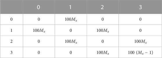
TABLE 3. GLCM for Mx wavelengths is similar to Figure 3A1 with a horizontal displacement vector d =(Δy, Δx)=(0,1) or d =(0,−1).

TABLE 4. Normalized GLCM of Table 3 entries for Mx wavelengths shown in Figure 3A1 with a horizontal displacement vector d = (Δy, Δx) = (0,1) or d = (0, −1).
3.2.2.2.3 Random reshuffling of pixels
For a random reshuffling of pixels in the synthetic image, we expect
In summary, the upper bound of the contrast is always
3.2.4 Bound estimates for correlation feature
3.2.4.1 Bit depth reduction effect on correlation
A cursory inspection of Eq. 10 shows a dramatic decrease in the correlation feature f3 by bit depth reduction. For example, the un-normalized correlation sum is
3.2.4.2 Lower and upper bounds for correlation
3.2.4.2.1 Vertical displacement vectors
For a one-unit vertical displacement vector in the vertically striped images shown in Figure 3, the only entries in GLCM are along the main diagonal such that p(i, i) = (Ny − 1)/((Ny − 1)Nx) = 1/Nx. Because of the GLCM symmetry, the x-direction marginal probability distribution px(i) and for y-direction py(i) are equal at
3.2.4.2.2 Horizontal displacement vectors
To further simplify the calculations, one assumes that the image has a one gray-level per pixel gradient along the x-direction (Figure 3). To further simplify the evaluation of the correlation for periodic patterns shown in Figure 3, we only consider one period, Mx = 1 in Table 4. As a result, the marginal probabilities are px = py = (1, 2, … , 2, 1), and the non-zero GLCM entries are aligned only along the two symmetric contrast lines k = j − i = ±1 with equal probability
The un-normalized correlation sum is
3.2.4.2.3 Random reshuffling of pixels
Randomly reshuffling of the pixels in an image
In summary, the lower bound of the correlation is always 0, as seen from Section 3.2.4.2.3. The upper bound of f3 depends on the specific patterns. For uniform patterns, such as Figure 3 along the vertical displacement vector, the correlation feature is a maximum of f3, max = 1, as shown in Section 3.2.4.2.1. For periodic patterns, such as those shown in Figure 3 along the horizontal displacement vector, the correlation feature depends on the gray-level quantization (or the wavelength of the pattern) and is
While theoretical estimates can be derived for any other Haralick feature, as shown previously, entropy is the only other feature of interest.
3.2.5 Bound estimates for entropy feature
3.2.5.1 Bit depth reduction effect on entropy
According to Eq. 16, 1-bit GLCM is
3.2.5.2 Lower and upper bounds for entropy
3.2.5.2.1 Vertical displacement vectors
Since a vertical displacement vector in a vertically striped image, such as those shown in Figures 4A1, B1, only determines diagonal entries in GLCM as in Figure 3C1, we first consider the simplest possible case of a one gray level per pixel gradient, which means that all diagonal entries are equal and
3.2.5.2.2 Horizontal displacement vectors
For horizontal displacement vectors in a vertically striped image, such as those in Figures 4A1, B1, with a gradient of one gray level per pixel, GLCM has elements parallel to the main diagonal (Figure 3C1). For an 8-bit image, the non-zero elements of GLCM should be
3.2.5.2.3 Random reshuffling of pixels
As with the previous Haralick features, for a random reshuffling of the pixels in an image
In summary, the upper bound of the entropy is always
Figure 6 shows all 14 Haralick features, of which we have discussed in detail only the four most relevant for the patterns shown in Figures 3, 4. All plots are on a semi-log horizontal scale, showing the results for horizontal and vertical unit displacement vectors.
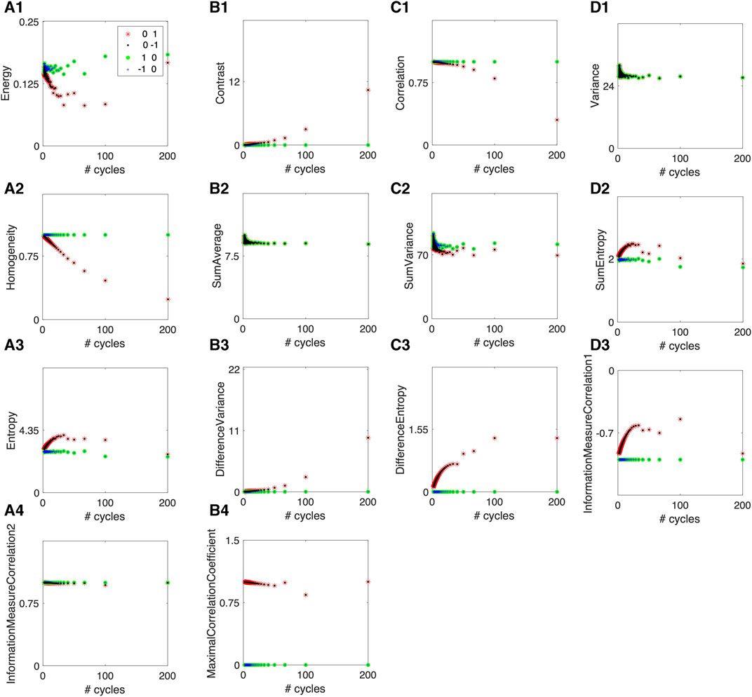
FIGURE 6. Complete set of 14 Haralick features for vertical stripes. The 14 original Haralick features (see definitions in Section 2) are plotted on a horizontal semi-log axis vs. the number of repeating cycles of one wavelength (Figure 3). The horizontal displacement vectors d =(Δy, Δx)=(0,1) to the right of the current pixel location (red stars) and d =(0,−1) to the left (solid black squares), and the vertical displacement d =(1,0) downward (green solid circle) and d =(1−,0) upward (blue cross) measure features along the respective directions. (A1) The image has no gradients along the vertical directions, and, therefore, the energy (A1) is constant regardless of the number of cycles of gradients along the horizontal direction. Similarly, the contrast (B1) is zero, and the correlation (C1) is maximum along the vertical directions. The variance (D1), the sum average (B2), the information measure of correlation 2 (A4), and the sum variance (C2) are not quite sensitive to the displacement vector direction in this particular type of pattern. The homogeneity (A2) is constant and maximum possible along the vertical directions. The sum entropy (D2), entropy (A3), Difference entropy (C3), and information measure of correlation 1 (D3) are all constant along vertical displacements and show an exponential increase with the number of cycles along the periodic horizontal pattern. Eventually, these features saturate as the number of cycles increases due to the space GLCM structure. The variance difference (B3) and the maximum correlation coefficient (B4) are both zero for the uniform gray levels along the vertical displacement vector and sensitive to periodic gradients along the horizontal direction.
The values of the Haralick features in Figure 7 are provided as references. As expected, there are many redundant features, so we have only focused on four. For example, the inverse difference momentum (IDM) of homogeneity featuring f5 in Figure 6A2 is an inverse measure to the contrast discussed in detail in Figure 5B1 (see also Figure 6B1).
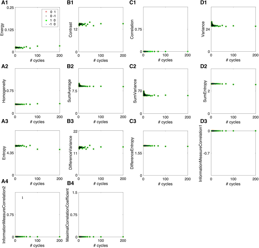
FIGURE 7. Complete set of 14 Haralick features for a random reshuffle of the vertically striped images. The 14 original Haralick features shown in Figure 6 have reference values corresponding to a random reshuffle of all pixels. (A1) The energy for randomly reshuffling the pixels in the image has a lower value than for the periodic patterns in Figure 6A1. The contrast (B1) of reshuffling the pixels gives the upper bound over all pixel arrangements. The correlation (C1) among pixels is totally lost by randomly reshuffling the pixels. The variance (D1) and the sum average (B2) are not particularly useful for the type of patterns considered in this study. The homogeneity (A2) reaches its lower bound for randomly reshuffled pixels, asymptotically approached by the periodic gradients (see Figure 6A2). The sum variance (C2) reaches its lower bound for randomly reshuffled pixels. All entropy-related measures such as sum entropy (D2), entropy (A3), and difference entropy (C3) are maximum for randomly reshuffled pixels, and they correspond to asymptotic values of the respective features in periodic gradients (see Figures 6A3, D2, C3, respectively). The difference variance (B3) is the maximum possible, and the information measure of correlation 1 (D3), the information measure of correlation 2 (A4), and the maximum correlation coefficient (B4) are all zero for randomly reshuffled pixels. These values are also bounds which the respective features approach asymptotically for periodic gradients (see the corresponding panels in Figure 6).
To avoid cluttering the plots, we also show the same features in Figure 7 after randomly reshuffling the pixels in the original images. We also notice from Figure 7 that the Haralick feature has the same value regardless of the direction of the unit displacement vector.
4 Conclusion
One of the main difficulties in using GLCM and Haralick features, as opposed to Fourier-based spectral methods in signal and image processing, is the fact that the real space mapping of the original signal is lost. Indeed, for example, the Fourier space of a two-dimensional image I(y, x) is a conjugate space i(qy, qx) where the wavenumber qx = 2π/λ is directly related to the spatial size λ of the pattern in the image. Therefore, the Fourier spectrum allows direct mapping of the results back into the image space. Since GLCM and the corresponding Haralick features retain only a relative arrangement of gray-level intensities in an image, they only encode gray-level gradients present in images. While GLCM has the advantage of a simpler interpretation than Fourier spectral analysis, its most significant shortcoming is the quadratic
We found that the structure of GLCM directly encoded the gray-level intensity gradients along a given direction in the image (Section 3.1). In our synthetic images (Figures 3A1, A2, 4A, B) of vertical stripes, the vertical direction has uniform gray levels—zero gradients. We found that a zero gradient along a given direction generates only entries along the main, or principal, diagonal of GLCM for the respective gray level. Each entry along the main diagonal measures the pattern’s size along the displacement vector and its width perpendicular to it. For example, one vertical stripe of gray level 0 with a length of Ny = 100 pixels generates the GLCM entry P(0, 0) = (Ny − 1) = 99 when measured along a vertical displacement vector. If the gray level stripe has a width of w = 2, then the GLCM entry becomes w (Ny − 1) = 198. However, because GLCM does not preserve information about the spatial location of image pixels, it cannot be determined whether the w (Ny − 1) GLCM entry was determined by a single stripe with wNy pixels or by w stripes, each with Ny pixels.
Similarly, we found that a gradient of one gray level per pixel produces only GLCM entries along the first parallel lines to the main diagonal of GLCM (Section 3.1). Furthermore, a positive gradient of one gray level per pixel along the horizontal displacement vector produces GLCM entries that rotate clockwise, such as p(1, 2), followed by p(2, 3), then by p(3, 4), and so on, and they are arranged above the main diagonal. A gradient of two gray levels per pixel will generate GLCM entries along the second parallel lines from the main diagonal.
We also found that bit depth reduction generates diagonal entries in GLCM. Bit depth reduction occurs, for example, during data compression. GLCM cannot distinguish between the effect of bit depth reduction, which blurs the image, versus actual uniform gray-level patches present in the original image. Furthermore, since GLCM is a lower dimensional
Haralick features reduce the data dimensionality from the
All four Haralick features analyzed in detail were analytically estimated for uniform random distribution of pixels across the entire image with a given
Bit depth reduction produces a block shrinking of GLCM similar to a convolution (Figures 3C1, C2). The only difference is that, while convolutions have an odd-size kernel such that they can compute a replacement for the central value based on the neighboring values, a 1-bit depth reduction of GLCM always operates on gray-level values as a 2 × 2 kernel by dropping the least significant bit (Eq. 22).
On the other hand, we found that the gray level quantization of the periodic sin (2πx/λ) for different values of λ produces power–law dependence, such as Eq. 23 (curve ‘A’ in Figure 4D) and Eq. 24 (curve ‘B’ in Figure 4D). Consequently, such power–law dependencies on λ or, equivalently, on the number of cycles Mx = Nx/λ were observed in the four analyzed Haralick features (Figures 5A1–D1) when plotted against the number of cycles.
We provided bounds for Haralick features for the synthetic gradient pattern, allowing a straightforward interpretation of the results for future applications. As real-world textures are more complex than the gradients investigated here, our findings could be generalized and integrated into a systematic approach to the meaningful use of Haralick features for image processing.
Data availability statement
The original contributions presented in the study are included in the article/Supplementary material; further inquiries can be directed to the corresponding author.
Author contributions
AO: conceptualization, data curation, formal analysis, funding acquisition, investigation, methodology, project administration, resources, software, supervision, validation, visualization, writing–original draft, and writing–review and editing. SO: conceptualization, data curation, formal analysis, funding acquisition, investigation, methodology, project administration, resources, software, supervision, validation, visualization, writing–original draft, and writing–review and editing.
Funding
The author(s) declare financial support was received for the research, authorship, and/or publication of this article: the South Carolina Space Grant Consortium partially supported this research. Department of Physics and Astronomy at the College of Charleston covered the publication cost.
Conflict of interest
The authors declare that the research was conducted in the absence of any commercial or financial relationships that could be construed as a potential conflict of interest.
Author SO declared that they were an editorial board member of Frontiers at the time of submission. This had no impact on the peer review process and final decision.
Publisher’s note
All claims expressed in this article are solely those of the authors and do not necessarily represent those of their affiliated organizations, or those of the publisher, the editors, and the reviewers. Any product that may be evaluated in this article, or claim that may be made by its manufacturer, is not guaranteed or endorsed by the publisher.
References
Abe, K., Minami, M., Miyazaki, R., and Tian, H. (2014). Application of a computer-aid diagnosis of pneumoconiosis for cr x-ray images. J. Biomed. Eng. Med. Imaging 1. doi:10.14738/jbemi.15.606
Akhter, Y., Singh, R., and Vatsa, M. (2023). AI-based radiodiagnosis using chest X-rays: a review. Front. Big Data 6, 1120989. doi:10.3389/fdata.2023.1120989
Araujo, A. S., Conci, A., Moran, M. B. H., and Resmini, R. (2018). “Comparing the use of sum and difference histograms and gray levels occurrence matrix for texture descriptors,” in 2018 International Joint Conference on Neural Networks (IJCNN), Rio de Janeiro, Brazil, July 8-13, 2018, 1–8. doi:10.1109/IJCNN.2018.8489705
Azami, H., da Silva, L. E. V., Omoto, A. C. M., and Humeau-Heurtier, A. (2019). Two-dimensional dispersion entropy: an information-theoretic method for irregularity analysis of images. Signal Process. Image Commun. 75, 178–187. doi:10.1016/j.image.2019.04.013
Baldini, G., Giuliani, R., Steri, G., and Neisse, R. (2017). “Physical layer authentication of Internet of Things wireless devices through permutation and dispersion entropy,” in 2017 Global Internet of Things Summit (GIoTS), Geneva, Switzerland, 06-09 June 2017, 1–6. doi:10.1109/GIOTS.2017.8016272
Baldini, G., Hernandez Ramos, J. L., and Amerini, I. (2021). Intrusion detection based on gray-level co-occurrence matrix and 2d dispersion entropy. Appl. Sci. 11, 5567. doi:10.3390/app11125567
Bodalal, Z., Trebeschi, S., Nguyen-Kim, T. D. L., Schats, W., and Beets-Tan, R. (2019). Radiogenomics: bridging imaging and genomics. Abdom. Radiol. 44, 1960–1984. doi:10.1007/s00261-019-02028-w
Cao, W., Pomeroy, M. J., Zhang, S., Tan, J., Liang, Z., Gao, Y., et al. (2022). An adaptive learning model for multiscale texture features in polyp classification via computed tomographic colonography. Sensors (Basel) 22, 907. doi:10.3390/s22030907
Chang, J., Xiao, Y., and Zhang, Z. (2019). “Wireless physical-layer identification assisted 5g network security,” in 2019 - IEEE Conference on Computer Communications Workshops (INFOCOM WKSHPS), Paris, France, 29 April - 2 May 2019, 1–5. doi:10.1109/INFOCOMWKSHPS47286.2019.9093751
Cook, G. J., Yip, C., Siddique, M., Goh, V., Chicklore, S., Roy, A., et al. (2013). Are pretreatment 18F-FDG PET tumor textural features in non-small cell lung cancer associated with response and survival after chemoradiotherapy? J. Nucl. Med. 54, 19–26. doi:10.2967/jnumed.112.107375
Criss, C., Nagar, A. M., and Makary, M. S. (2023). Hepatocellular carcinoma: State of the art diagnostic imaging. World J. Radiol. 15, 56–68. doi:10.4329/wjr.v15.i3.56
Devnath, L., Luo, S., Summons, P., Wang, D., Shaukat, K., Hameed, I. A., et al. (2022). Deep ensemble learning for the automatic detection of pneumoconiosis in coal worker’s chest x-ray radiography. J. Clin. Med. 11, 5342. doi:10.3390/jcm11185342
El-Baz, A., Nitzken, M., Vanbogaert, E., Gimel’farb, G., Falk, R., and Abou-El-Ghar, M. (2011). A novel shape-based diagnostic approach for early diagnosis of lung nodules “in 2011 IEEE International Symposium on Biomedical Imaging: From Nano to Macro, Chicago, IL, USA, 30 March 2011 - 02 April, 137–140. doi:10.1109/ISBI.2011.5872373
Feng, L., Yang, X., Lu, X., Kan, Y., Wang, C., Sun, D., et al. (2022). (18)F-FDG PET/CT-based radiomics nomogram could predict bone marrow involvement in pediatric neuroblastoma. Insights Imaging 13, 144. doi:10.1186/s13244-022-01283-8
Ferro, M., Crocetto, F., Barone, B., Del Giudice, F., Maggi, M., Lucarelli, G., et al. (2023a). Artificial intelligence and radiomics in evaluation of kidney lesions: a comprehensive literature review. Ther. Adv. Urol. 15, 175628722311648. doi:10.1177/17562872231164803
Ferro, M., Musi, G., Marchioni, M., Maggi, M., Veccia, A., Del Giudice, F., et al. (2023b). Radiogenomics in renal cancer management-current evidence and future prospects. Int. J. Mol. Sci. 24, 4615. doi:10.3390/ijms24054615
Hall, E. L., Crawford, J. W. O., and Roberts, F. E. (1975). Computer classification of pneumoconiosis from radiographs of coal workers. IEEE Trans. Biomed. Eng. 22, 518–527. doi:10.1109/tbme.1975.324475
Haralick, R. (1979). Statistical and structural approaches to texture. Proc. IEEE 67, 786–804. doi:10.1109/PROC.1979.11328
Haralick, R. M., Shanmugam, K., and Dinstein, I. (1973). Textural features for image classification. IEEE Trans. Syst. Man, Cybern.SMC 3, 610–621. doi:10.1109/TSMC.1973.4309314
Humeau-Heurtier, A. (2019). Texture feature extraction methods: a survey. IEEE Access 7, 8975–9000. doi:10.1109/ACCESS.2018.2890743
Jeong, W. K., Jamshidi, N., Felker, E. R., Raman, S. S., and Lu, D. S. (2019). Radiomics and radiogenomics of primary liver cancers. Clin. Mol. Hepatol. 25, 21–29. doi:10.3350/cmh.2018.1007
Julesz, B. (1975). Experiments in the visual perception of texture. Sci. Am. 232, 34–43. doi:10.1038/scientificamerican0475-34
Karanja, E. M., Masupe, S., and Jeffrey, M. G. (2020). Analysis of Internet of Things malware using image texture features and machine learning techniques. Internet Things 9, 100153. doi:10.1016/j.iot.2019.100153
Kratz, L., and Nishino, K. (2012). Tracking pedestrians using local spatio-temporal motion patterns in extremely crowded scenes. IEEE Trans. Pattern Anal. Mach. Intell. 34, 987–1002. doi:10.1109/tpami.2011.173
Kruger, R. P., Thompson, W. B., and Turner, A. F. (1974). Computer diagnosis of pneumoconiosis. IEEE Trans. Syst. Man, Cybern.SMC 4, 40–49. doi:10.1109/TSMC.1974.5408519
Lloyd, K., Rosin, P. L., Marshall, D., and Moore, S. C. (2017). Detecting violent and abnormal crowd activity using temporal analysis of Grey Level Co-occurrence Matrix (GLCM)-based texture measures. Mach. Vis. Appl. 28, 361–371. doi:10.1007/s00138-017-0830-x
Lofstedt, T., Brynolfsson, P., Asklund, T., Nyholm, T., and Garpebring, A. (2019). Gray-level invariant Haralick texture features. PLOS ONE 14, e0212110–e0212118. doi:10.1371/journal.pone.0212110
Lunt, T. F. (1993). A survey of intrusion detection techniques. Comput. Secur. 12, 405–418. doi:10.1016/0167-4048(93)90029-5
Mallat, S. G. (1989). A theory for multiresolution signal decomposition: the wavelet representation. IEEE Trans. Pattern Anal. Mach. Intell. 11, 674–693. doi:10.1109/34.192463
McNitt-Gray, M. F., Wyckoff, N., Sayre, J. W., Goldin, J. G., and Aberle, D. R. (1999). The effects of co-occurrence matrix based texture parameters on the classification of solitary pulmonary nodules imaged on computed tomography. Comput. Med. Imaging Graph 23, 339–348. doi:10.1016/s0895-6111(99)00033-6
Naik, A. J., and Gopalakrishna, M. (2017). Violence detection in surveillance video - a survey. Int. J. Latest Res. Eng. Technol. (IJLRET) 1, 1–17.
Nakata, N., and Siina, T. (2023). Ensemble learning of multiple models using deep learning for multiclass classification of ultrasound images of hepatic masses. Bioeng. (Basel) 10, 69. doi:10.3390/bioengineering10010069
Permuth, J. B., Choi, J., Balarunathan, Y., Kim, J., Chen, D. T., Chen, L., et al. (2016). Combining radiomic features with a miRNA classifier may improve prediction of malignant pathology for pancreatic intraductal papillary mucinous neoplasms. Oncotarget 7, 85785–85797. doi:10.18632/oncotarget.11768
Preparata, F. P., and Sarwate, D. V. (1977). Computational complexity of Fourier transforms over finite fields. Math. Comput. 31, 740–751. doi:10.1090/s0025-5718-1977-0436662-8
Prinzi, F., Militello, C., Conti, V., and Vitabile, S. (2023). Impact of wavelet kernels on predictive capability of radiomic features: a case study on Covid-19 chest x-ray images. J. Imaging 9, 32. doi:10.3390/jimaging9020032
Raman, S. P., Chen, Y., Schroeder, J. L., Huang, P., and Fishman, E. K. (2014). Ct texture analysis of renal masses: pilot study using random forest classification for prediction of pathology. Acad. Radiol. 21, 1587–1596. doi:10.1016/j.acra.2014.07.023
Raman, S. P., Schroeder, J. L., Huang, P., Chen, Y., Coquia, S. F., Kawamoto, S., et al. (2015). Preliminary data using computed tomography texture analysis for the classification of hypervascular liver lesions: generation of a predictive model on the basis of quantitative spatial frequency measurements–a work in progress. J. Comput. Assist. Tomogr. 39, 383–395. doi:10.1097/rct.0000000000000217
Ryan, D., Denman, S., Fookes, C., and Sridharan, S. (2011). “Textures of optical flow for real-time anomaly detection in crowds,” in 2011 8th IEEE International Conference on Advanced Video and Signal Based Surveillance (AVSS), Klagenfurt, 30 2011 to Sept. 2 2011, 230–235. doi:10.1109/AVSS.2011.6027327
Serrano Gracia, I., Deniz Suarez, O., Bueno Garcia, G., and Kim, T. K. (2015). Fast fight detection. PLOS ONE 10 (4), e0120448. doi:10.1371/journal.pone.0120448
Sivarajasingam, V., Shepherd, J. P., and Matthews, K. (2003). Effect of urban closed circuit television on assault injury and violence detection. Inj. Prev. 9, 312–316. doi:10.1136/ip.9.4.312
Song, B., Zhang, G., Lu, H., Wang, H., Zhu, W., Pickhardt, J. P., et al. (2014). Volumetric texture features from higher-order images for diagnosis of colon lesions via CT colonography. Int. J. Comput. Assist. Radiol. Surg. 9, 1021–1031. doi:10.1007/s11548-014-0991-2
Soufi, M., Arimura, H., and Nagami, N. (2018). Identification of optimal mother wavelets in survival prediction of lung cancer patients using wavelet decomposition-based radiomic features. Med. Phys. 45, 5116–5128. doi:10.1002/mp.13202
Voorthuijsen, G., Hoof, H., Klima, M., Roubik, K., Bernas, M., and Pata, P. (2005). “Cctv effectiveness study,” in Proceedings 39th Annual 2005 International Carnahan Conference on Security Technology, Las Palmas, Spain, 11-14 October 2005, 105–108. doi:10.1109/CCST.2005.1594815
Wang, J., and Xu, Z. (2016). Spatio-temporal texture modelling for real-time crowd anomaly detection. Comput. Vis. Image Underst. 144, 177–187. doi:10.1016/j.cviu.2015.08.010
Wang, S., Zhou, L., Li, X., Tang, J., Wu, J., Yin, X., et al. (2022). A novel deep learning model to distinguish malignant versus benign solid lung nodules. Med. Sci. Monit. 28, e936830. doi:10.12659/msm.936830
Keywords: sinusoidal gradient, Haralick features, bit depth reduction, constant gradient, image processing, signal processing, gray-level co-occurrence matrix
Citation: Oprisan A and Oprisan SA (2023) Bounds for Haralick features in synthetic images with sinusoidal gradients. Front. Sig. Proc. 3:1271769. doi: 10.3389/frsip.2023.1271769
Received: 02 August 2023; Accepted: 20 October 2023;
Published: 23 November 2023.
Edited by:
Antonia Papandreou-Suppappola, Arizona State University, United StatesReviewed by:
Malaya Kumar Nath, National Institute of Technology Puducherry, IndiaDenis Stanescu, Université Grenoble Alpes, France
Copyright © 2023 Oprisan and Oprisan. This is an open-access article distributed under the terms of the Creative Commons Attribution License (CC BY). The use, distribution or reproduction in other forums is permitted, provided the original author(s) and the copyright owner(s) are credited and that the original publication in this journal is cited, in accordance with accepted academic practice. No use, distribution or reproduction is permitted which does not comply with these terms.
*Correspondence: Ana Oprisan, b3ByaXNhbmFAY29mYy5lZHU=