Doppler frequency analysis for sound-field sampling with moving microphones

Moving microphones allow for the fast acquisition of sound-field data that encode acoustic impulse responses in time-invariant environments. Corresponding decoding algorithms use the knowledge of instantaneous microphone positions for relating the dynamic samples to a positional context and solving the involved spatio-temporal channel estimation problem subject to the particular parameterization model. Usually, the resulting parameter estimates are supposed to remain widely unaffected by the Doppler effect despite the continuously moving sensor. However, this assumption raises issues from the physical point of view. So far, mathematical investigations into the actual meaning of the Doppler effect for such dynamic sampling procedures have been barely provided. Therefore, in this paper, we propose a new generic concept for the dynamic sampling model, introducing a channel representation that is explicitly based on the instantaneous Doppler shift according to the microphone trajectory. Within this model, it can be clearly seen that exact trajectory tracking implies exact Doppler-shift rendering and, thus, enables unbiased parameter recovery. Further, we investigate the impact of non-perfect trajectory data and the resulting Doppler-shift mismatches. Also, we derive a general analysis scheme that decomposes the microphone signal along with the encoded parameters into particular subbands of Doppler-shifted frequency components. Finally, for periodic excitation, we exactly characterize the Doppler-shift influences in the sampled signal by convolution operations in the frequency domain with trajectory-dependent filters.

1 Introduction

Dynamic measurement procedures are capable of acquiring entire sound-field information by use of only one non-stop moving microphone. Due to their low effort in hardware and calibration compared to stationary approaches, such continuous techniques are ideally suited to gather fast estimates of acoustic impulse responses (AIRs) within expanded listening areas. Prominent examples of AIRs are head-related impulse responses (HRIRs), room impulse responses (RIRs), and binaural room impulse responses (BRIRs). Adequate estimates of AIR fields are essential for various applications related to multichannel equalization and cross-talk cancellation, sound-field analysis, auralization, and audio reproduction, e.g., for virtual and augmented reality systems (Benesty et al., 2008).

An analytical method for the reconstruction of AIRs along linear and circular microphone trajectories has been presented in (Ajdler et al., 2007). Here, a specially designed input signal is needed, and the speed of the microphone must be constant and is restricted to an upper limit. Quite different from usual AIR measurements, the excitation signal must not contain all audio frequencies, but only a certain subset in order to avoid overlapping frequency shifts. The omitted frequencies are essentially generated through the Doppler effect. Beyond that method, dynamic approaches are typically based on estimates from linear equations that model the convolution of involved AIRs and excitation sequences, and relate them to the samples acquired at instantaneously varying microphone positions. In one group of such methods, the spatio-temporal dependencies are simplified and impulse responses at steadily changing positions are considered as time-varying systems whose coefficients are tracked by adaptive filtering concepts (Haykin, 2001). This setup is well-known from acoustic echo cancellation (Sondhi, 1967; Benesty et al., 2006), and, combined with controlled surroundings and trajectories, it is also suitable for the fast acquisition of HRIRs (Enzner, 2008; He et al., 2018).

More recently, a new group of dynamic techniques have emerged, where the continuously acquired sound-field samples are directly embedded into a spatio-temporal context (Hahn and Spors, 2016; Katzberg et al., 2017b, 2018, 2021; Hahn et al., 2017; Hahn and Spors, 2017; Hahn and Spors, 2018; Urbanietz and Enzner, 2020). Here, the measurement model is explicitly multidimensional, with a moving microphone that collects uniform samples in the time domain and, in general, non-uniform samples at varying points in the spatial domain. Thus, such techniques inherently require positional information based either on a controlled pre-defined trajectory or a tracking of the microphone positions (Katzberg et al., 2022). The method by Urbanietz and Enzner (2020) uses a spatial Fourier basis for the angular reconstruction of HRIRs from continuous-azimuth recordings and shows more accurate performance than an adaptive-filter-based solution. In (Hahn and Spors, 2016), perfect-sequence excitation (Stan et al., 2002) is used for the orthogonal expansion of impulse responses, in order to describe the dynamic spatio-temporal sampling by notional static sampling processes of single expansion coefficients. This method simplifies the problem to pure interpolation in space. It has been investigated for reconstructing RIRs (Hahn and Spors, 2017; Hahn and Spors, 2018) and BRIRs (Hahn et al., 2017) along circular trajectories. In (Katzberg et al., 2017b), a versatile framework has been presented that allows for RIR reconstruction at off-trajectory positions within cubical volumes. To achieve this, the sound field is parameterized by modeling virtual grid points in space, and dynamic samples are understood as the result of bandlimited interpolation on that grid using sampled sinc-function approximations. In practice, the corresponding inverse problem is most likely ill-posed or even underdetermined. Therefore, in (Katzberg et al., 2018; Katzberg and Mertins, 2022), a strategy has been proposed that exploits sparse Fourier representations and applies principles of compressed sensing (CS) (Candès et al., 2006). Recently, the dynamic framework subject to sinc-function related parameters has been generalized to a formulation, where arbitrary spatial basis functions cover expanded target volumes (Katzberg et al., 2021). Based on this, a physical perspective has been provided for representing dynamic sound-field samples in terms of spherical solutions to the acoustic wave equation (Katzberg et al., 2021).

For the measurement methods where a non-stop moving microphone collects sound-field data to AIRs, the Doppler effect will always be present in the sampled signal. The dynamic approaches considering the spatio-temporal context rely on the assumption that the occurring Doppler shifts are at least partly covered by the sampling model, as long as the microphone signal at the particular receiving times is connected to the instant positions in space. However, for all the existing frameworks, the implication between positional tracking and Doppler-shift rendering is not directly apparent from the mathematical model. Therefore, in this paper, we introduce a new interpretation of the dynamic sampling procedure from the Doppler perspective.

First, in Section 2, we briefly outline the basic differences in the mathematical models between stationary and dynamic sound-field measurement strategies. Then, in Section 3, we develop an equivalent Doppler-domain concept from which one can easily see that exact tracking of the microphone trajectory inherently allows for the exact tracking of the involved and unknown Doppler shifts in the frequency domain. The proposed representation explicitly describes the instantaneous interferences of the Doppler effect during the dynamic observation process. This can be used to estimate the underlying sound-field parameters without any Doppler bias, provided that the acoustic properties of the surroundings remain constant during the measurement sessions. In Section 4, we analyze the case of non-perfect positional tracking and describe the resulting Doppler-shift mismatches in the mathematical model. We derive structured expressions for the corresponding error terms and adapt stability guarantees and error bounds for both least-squares and CS-based solutions. In Section 5, the Doppler-based channel representation is exploited to provide a spatio-temporal filtering scheme that can be employed for decomposing the Doppler-shifted microphone signal into particular subbands. This allows us to reconstruct low-frequency content in cases where the wideband recovery problem is ill-conditioned. Considering periodic excitation, Section 6 shows how the proposed concept enables us to directly relate the Doppler shifts in the measured signal to trajectory-dependent filters that spread spectral sound-field characteristics across adjoining frequency bins. Finally, in Section 7, we demonstrate the key points of the Doppler framework on experimental data.

2 Dynamic sound-field sampling procedures

Assuming a fixed environment with several reflecting surfaces and constant atmospheric conditions, the propagation of the sound signal s(t) inside the target area $\mathrm{\Omega }\subset {\mathbb{R}}^3$ can be considered as a linear time-invariant (LTI) system. This leads to the observation model

$p\left(\mathit{x},t\right)={\int }_{-\infty }^{\infty }s\left(t-\tau \right)h\left(\mathit{x},\tau \right)\mathrm{d}\tau ,(1)$

where s(t) originates at a fixed source position x_S∉Ω subject to the global time $t\in \mathbb{R}$, p(x, t) is the observed sound-pressure field depending on the receiver position x = [x,y,z]^T ∈ Ω in Cartesian coordinates, and h(x, τ) is the spatio-temporal AIR subject to the delay time τ. The AIR describes the particular LTI system, i.e., the sound field for a Dirac impulse excitation at τ = 0.

By coupling the spatial dimensions to the time dimension, the dynamic sound field along the trajectory $\tilde{\mathit{x}}(t)={[\tilde{x}(t),\tilde{y}(t),\tilde{z}(t)]}^T$, defined by the time-dependent motion function ${\tilde{\mathit{x}}}_t:\mathbb{R}\to \tilde{\mathrm{\Omega }}$, is observed as

$\tilde{p}\left(\tilde{\mathit{x}}\left(t\right),t\right)={\int }_{-\infty }^{\infty }s\left(t-\tau \right)h\left(\tilde{\mathit{x}}\left(t\right),\tau \right)\mathrm{d}\tau ,(2)$

where $h(\tilde{\mathit{x}}(t),\tau )$ represents the spatio-temporal AIR within the trajectory space $\tilde{\mathrm{\Omega }}\subseteq \mathrm{\Omega }$. In the following subsections, we briefly compare the general concepts of stationary and dynamic sound-field sampling strategies.

2.1 Stationary sampling schemes

Measuring the sound-field signal (1) leads to stationary sampling schemes, where R microphones provide temporal samples with high acquisition rates f_s at uniform points t_n = n/f_s $(n\in \mathbb{Z})$, and, in general, spatial samples at N non-uniform positions x_r (r ∈ {1, …, N}) inside the volume of interest Ω. Strategies for the sampling and reconstruction in space are generally based on an appropriate parametrization of the continuous-space and discrete-time AIR within bounds of Ω,

$h\left(\mathit{x},m\right)\approx {\displaystyle \sum _{l=0}^{L-1}}{\displaystyle \sum _{c=0}^{C-1}}\gamma \left(c,l\right)f\left(c,\mathit{x}\right)g\left(l,m\right),(3)$

where f(c, x) are sampled basis functions for the interpolation inside Ω according to a spatialization model (e.g., sampled plane waves), $g$(l, m) are basis functions for the sampled delay time dimension m (e.g., discrete Fourier basis), and γ(c, l) are the corresponding sound-field parameters, i.e., coefficients describing the AIR field h(x, m). For h(x_r, m) vanishing into the noise level at m ≥ L, the parameters are encoded in spatio-temporal samples of (1) subject to

$\begin{array}{cc}\hfill p\left({\mathit{x}}_r,n\right)& ={\displaystyle \sum _{m=0}^{L-1}}s\left(n-m\right)h\left({\mathit{x}}_r,m\right)+{\eta }_r\left(n\right)\hfill \\ \hfill & ={\displaystyle \sum _{m=0}^{L-1}}s\left(n-m\right){\displaystyle \sum _{l=0}^{L-1}}{\displaystyle \sum _{c=0}^{C-1}}\gamma \left(c,l\right)f\left(c,{\mathit{x}}_r\right)g\left(l,m\right)+{\eta }_r\left(n\right),\hfill \end{array}(4)$

with η_r(n) comprising the measurement noise and parameterization errors. Parameter decoding may be achieved by solving the inverse problem given a controlled excitation sequence s(n) and calibrated sampling positions x_r. Adequate estimates of γ(c, l) from the corresponding system of linear equations may be used for the sound-field reconstruction according to (3). The reconstruction along the delay time m is simple due to high temporal sampling rates f_s ≥ 2f_cut of the microphones, effortlessly achievable for practical cutoff frequencies f_cut. Note that, of course, stationary microphones allow for decoupling the multidimensional sampling problem (4). So, in practice, estimates of h(x_r, m) are calculated first by solving the deconvolution problem for each microphone position separately, and then the parameters γ(c, l) are recovered from the remaining linear interpolation equations of the form $h({\mathit{x}}_r,m)={\displaystyle {\sum }_{l=0}^{L-1}}{\displaystyle {\sum }_{c=0}^{C-1}}\gamma (c,l)f(c,{\mathit{x}}_r)g(l,m)$.

2.2 Dynamic sampling schemes

For the sampling of the dynamic sound pressure (2), measurement procedures with moving microphones can be used that generate samples at uniform points in time and, generally, at continuously varying and non-uniform positions in space. As temporal sampling implies spatial sampling in such setups, only one microphone measuring along an appropriate trajectory $\tilde{\mathit{x}}(n)$ is sufficient for gathering the entire sound-field information. At this, the speed of the microphone is arbitrary and may vary, pausing is not required.

By employing the identical parameterization model as in (3), the spatio-temporal AIR sampled (non-uniformly) along the trajectory $\tilde{\mathit{x}}(n)\in \tilde{\mathrm{\Omega }}$ reads

$h\left(\tilde{\mathit{x}}\left(n\right),m\right)\approx {\displaystyle \sum _{l=0}^{L-1}}{\displaystyle \sum _{c=0}^{C-1}}\gamma \left(c,l\right)f\left(c,\tilde{\mathit{x}}\left(n\right)\right)g\left(l,m\right).(5)$

Accordingly, the particular sound-field parameters γ(c, l) are encoded in samples of (2) subject to

$\begin{array}{cc}\hfill \tilde{p}\left(\tilde{\mathit{x}}\left(n\right),n\right)& ={\displaystyle \sum _{m=0}^{L-1}}s\left(n-m\right)h\left(\tilde{\mathit{x}}\left(n\right),m\right)+\tilde{\eta }\left(n\right)\hfill \\ \hfill & ={\displaystyle \sum _{m=0}^{L-1}}s\left(n-m\right){\displaystyle \sum _{l=0}^{L-1}}{\displaystyle \sum _{c=0}^{C-1}}\gamma \left(c,l\right)f\left(c,\tilde{\mathit{x}}\left(n\right)\right)g\left(l,m\right)+\tilde{\eta }\left(n\right),\hfill \end{array}(6)$

where $\tilde{\eta }(n)$ encapsulates the errors due to sampling and finite-dimensional parameterization. Note, because $\tilde{\mathrm{\Omega }}\subseteq \mathrm{\Omega }$, the sampling model (6) may use the very same parameters and basis functions as the static model (4). However, in (6), the sampling of the spatial component is coupled to the global time index n subject to $f(c,\tilde{\mathit{x}}(n))$, since the involved AIR is immediately varying during the dynamic measurement process. The controlling of s(n) and tracking of $\tilde{\mathit{x}}(n)$ allow for estimates of γ(c, l) from the linear equations provided by (6) at time points $n=0,...,M-1$ and for the spatial reconstruction inside Ω according to (3). For high-speed movements, the noise level can be increased by air-flow perturbations in practice.

In fact, it turns out that all spatio-temporal sampling procedures with moving microphones as outlined in Section 1 are based on the sampling model (6), generally involving non-uniformly sampled basis functions $f(c,\tilde{\mathit{x}}(n))$ for the spatial dimensions and uniformly sampled basis functions $g$(l, m) for the temporal delay. Various dynamic strategies for recovering AIRs only differ in the specific choice of basis functions, i.e., the parameter representation of the target sound field inside Ω. In any case, spatial components $f(c,\tilde{\mathit{x}}(n))$ are evaluated subject to the time-dependent microphone trajectory ${\tilde{\mathit{x}}}_n:\mathbb{Z}\to {\mathbb{R}}^D$ performed in an actually D-dimensional subspace $\tilde{\mathrm{\Omega }}\subseteq \mathrm{\Omega }$.

In (Urbanietz and Enzner, 2020), for example, the sound-field parameters γ(c, l) are HRIRs themselves, spatially expanded by circular harmonics of maximum order Q. This is equivalent to the choices f(c, ϕ(n)) = e^{j(c−Q)ϕ(n)} and $g$(l, m) = δ(m − l), where δ is the unit impulse function and $\varphi (n)\in \tilde{\mathrm{\Omega }}$ is an azimuthal trajectory, i.e., the number of considered spatial dimensions is D = 1. By contrast, the method by Hahn and Spors (2017) uses f(c, ϕ(n)) = φ(c, ϕ(n)) and $g$(l, m) = s(l − m), with φ being Lagrange basis polynomials and s being an L-shift cross-orthogonal excitation sequence that fulfills ${\displaystyle {\sum }_{m=0}^{L-1}}s(n-m)s(l-m)=\delta (l-n\mathrm{mod}L)$ and, thus, simplifies (6) significantly. While these approaches confine the AIR target area to the one-dimensional (circular) trajectory curve itself $(\mathrm{\Omega }=\tilde{\mathrm{\Omega }})$, the methods in (Katzberg et al., 2017b; Katzberg et al., 2018; Katzberg et al., 2021) scale up to D = 3 using three-dimensional basis functions $f(c,\tilde{\mathit{x}}(n))$ that cover entire listening volumes. This allows for modeling the dynamic sampling along arbitrarily shaped microphone trajectories.

In this paper, we introduce a mathematical framework exploiting a representation by $g$(l, m) = e^j2πlm/L, in order to investigate frequency shifts in the sampled signal due to the Doppler effect. The following Doppler-shift descriptions cover dynamic acquisition techniques for several AIR types that assume constant environmental conditions, i.e., AIR variations are solely due to positional variations of the microphone.

3 Doppler-shift model for dynamic channels

In dynamic approaches, the sound signal sampled by the moving microphone is always affected by the Doppler effect. This raises the question about the impact of the involved Doppler shifts on the estimates of the sound-field parameters. Numerical and real-word experiments to the dynamic approaches outlined in Section 1 indicate that the positional tracking of the microphone allows for the Doppler-shift tracking in the dynamic signal, and, in turn, for uncorrupted parameter estimates. Thus, the key of these dynamic techniques lies in the tracking or controlling of the receiver trajectory, e.g., by using a robot-guided microphone, or by performing a circular trajectory at constant speed and measuring the round-trip time of the moving microphone. However, from the mathematical perspective, such implicit Doppler-shift rendering by use of positional data may not be straightforwardly comprehensible from a general spatio-temporal signal description in line with (6). In order to close this conceptual gap, we propose a more intrinsic channel interpretation for the dynamic sampling model.

3.1 General model for Doppler-shifted sound observations

For a general analytical description of interfering Doppler shifts, we use a doubly-dispersive signal model and adopt the concept of Doppler-variant impulse responses and transfer functions (Bello, 1963). Such Doppler-domain representations are well-known from time-varying channels in wireless systems (Haykin and Liu, 2010; Hlawatsch and Matz, 2011; Grami, 2016), e.g., for underwater acoustic communications (Li and Preisig, 2007; Zeng and Xu, 2012).

For the moment, let us disregard the spatial context in (2). Accordingly, the dynamic time signal $\tilde{p}(\tilde{\mathit{x}}(t),t)$ may be described by

$\tilde{p}\left(t\right)={\int }_{-\infty }^{\infty }s\left(t-\tau \right)h\left(t,\tau \right)\mathrm{d}\tau ,(7)$

with h(t, τ) being the time-variant impulse response. The Fourier transforms of h(t, τ) along the particular dimensions yield, respectively, the Doppler-variant impulse response

$\mathcal{D}\left(\nu ,\tau \right)={\int }_{-\infty }^{\infty }h\left(t,\tau \right){\mathrm{e}}^{-\mathrm{j}\nu t}\mathrm{d}t,(8)$

which contains the variable ν denoting the Doppler shift, the time-variant transfer function

$\mathcal{T}\left(t,\omega \right)={\int }_{-\infty }^{\infty }h\left(t,\tau \right){\mathrm{e}}^{-\mathrm{j}\omega \tau }\mathrm{d}\tau ,(9)$

with angular frequency $\omega =2\pi f$, and the Doppler-variant transfer function

$\mathcal{U}\left(\nu ,\omega \right)={\int }_{-\infty }^{\infty }{\int }_{-\infty }^{\infty }h\left(t,\tau \right){\mathrm{e}}^{-\mathrm{j}\left(\nu t+\omega \tau \right)}\mathrm{d}t\mathrm{d}\tau .(10)$

The time-variant impulse response in (7) may be interpreted as the time-varying contribution from a continuum of scattering paths. By using the inverse Fourier transform of $\mathcal{D}(\nu ,\tau )$, the interfering Doppler shifts in (7) are revealed as

$\tilde{p}\left(t\right)=\frac{1}{2\pi }{\int }_{-\infty }^{\infty }{\int }_{-\infty }^{\infty }\mathcal{D}\left(\nu ,\tau \right)s\left(t-\tau \right){\mathrm{e}}^{\mathrm{j}\nu t}\mathrm{d}\nu \mathrm{d}\tau .(11)$

In (11), we can see that the signal arriving at the moving receiver is composed of a weighted superposition of time-delayed and frequency-shifted replicas of the source sequence s(t). The weighting $\mathcal{D}(\nu ,\tau )$ defines the contribution to $\tilde{p}(t)$ from a scattering path with delay τ. The channel is called doubly-dispersive as it involves both delay and frequency spreads due to both multipath signal propagation and time-varying behavior. By using the inverse Fourier transform of $\mathcal{U}(\nu ,\omega )$, (11) can also be expressed as

$\begin{array}{cc}\hfill \tilde{p}\left(t\right)& =\frac{1}{{\left(2\pi \right)}^2}{\int }_{-\infty }^{\infty }{\int }_{-\infty }^{\infty }{\int }_{-\infty }^{\infty }\mathcal{U}\left(\nu ,\omega \right)s\left(t-\tau \right){\mathrm{e}}^{\mathrm{j}\left(\nu t+\omega \tau \right)}\mathrm{d}\nu \mathrm{d}\omega \mathrm{d}\tau \hfill \\ \hfill & =\frac{1}{{\left(2\pi \right)}^2}{\int }_{-\infty }^{\infty }{\int }_{-\infty }^{\infty }s\left(t-\tau \right){\mathrm{e}}^{\mathrm{j}\omega \tau }\mathrm{d}\tau {\int }_{-\infty }^{\infty }\mathcal{U}\left(\nu ,\omega \right){\mathrm{e}}^{\mathrm{j}\nu t}\mathrm{d}\nu \mathrm{d}\omega \hfill \\ \hfill & =\frac{1}{2\pi }{\int }_{-\infty }^{\infty }{S}_t\left(\omega \right)\frac{1}{2\pi }{\int }_{-\infty }^{\infty }\mathcal{U}\left(\nu ,\omega \right){\mathrm{e}}^{\mathrm{j}\nu t}\mathrm{d}\nu \mathrm{d}\omega ,\hfill \end{array}(12)$

with $S_t(\omega )={\int }_{-\infty }^{\infty }s(t-\tau ){\mathrm{e}}^{\mathrm{j}\omega \tau }\mathrm{d}\tau$ representing the time-dependent Fourier transform of the source signal s(t). For obvious reasons, $\mathcal{D}(\nu ,\tau )$ and $\mathcal{U}(\nu ,\omega )$ are also referred to as delay-Doppler spreading function and frequency-Doppler spreading function, respectively. The Fourier relationships between the four fundamental functions h, $\mathcal{D}$, $\mathcal{T}$, and $\mathcal{U}$ are summarized in Figure 1. Each of such representations describes any linear time-variant system completely (Hlawatsch and Matz, 2011).

Figure 1

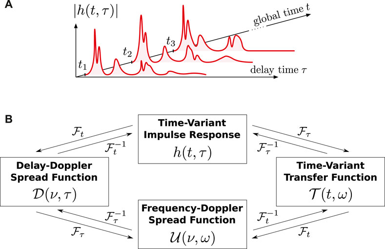
Figure 1. Linear time-variant channel impulse response. (A) Outline of considered dimensions and (B) particular frequency representations, where ${\mathcal{F}}_t$ denotes the Fourier transform along the variable t and ${\mathcal{F}}_t^{-1}$ is the corresponding inverse Fourier transform.

3.2 Spatial parameterization of the time-variant transfer function

In (12), the term ${(2\pi )}^{-1}{\int }_{-\infty }^{\infty }\mathcal{U}(\nu ,\omega ){\mathrm{e}}^{\mathrm{j}\nu t}\mathrm{d}\nu$ describes the time-varying channel as the interference of instantaneous Doppler shifts, where $\mathcal{U}(\nu ,\omega )$ parameterizes the frequency-dependent Doppler characteristics. The total effect of these characteristics could be considered unconnected, and, in general, estimated by adaptive filtering techniques that track the time-varying transfer function $\mathcal{T}(t,\omega )={(2\pi )}^{-1}{\int }_{-\infty }^{\infty }\mathcal{U}(\nu ,\omega ){\mathrm{e}}^{\mathrm{j}\nu t}\mathrm{d}\nu$. However, in contrast to, e.g., underwater acoustic channels where significant dynamics in the surrounding medium and scatterers are present, we assume a time-invariant configuration of scattering paths inside the target volume Ω. Accordingly, ${(2\pi )}^{-1}{\int }_{-\infty }^{\infty }\mathcal{U}(\nu ,\omega ){\mathrm{e}}^{\mathrm{j}\nu t}\mathrm{d}\nu$ is fully defined by the receiver trajectory within the LTI acoustic field H(x, ω). The acoustic field can be described by the general model

$H\left(\mathit{x},\omega \right)={\int }_{-\infty }^{\infty }A\left(\rho ,\omega \right)f\left(\rho ,\mathit{x}\right)\mathrm{d}\rho ,(13)$

where A(ρ, ω) is a continuum of sound-field parameters subject to the variable ρ that constitutes a continuum of possible spatial variations for x ∈ Ω due to multipath arrivals, and f(ρ, x) are appropriate spatial basis functions. The reverberant field H(x, ω) represents solutions to the Helmholtz equation for a Dirac impulse excitation at τ = 0. In the following descriptions, H(x, ω) is considered as the spatial transfer function from the static sound source to the receiver position x.

Doppler shifts can be represented in terms of the (unknown) acoustic field (13) with fixed initial and boundary conditions. By introducing the spatial context subject to H(x, ω), we rewrite the dynamic signal (12) as

$\tilde{p}\left(\tilde{\mathit{x}}\left(t\right),t\right)=\frac{1}{2\pi }{\int }_{-\infty }^{\infty }{S}_t\left(\omega \right)H\left(\tilde{\mathit{x}}\left(t\right),\omega \right)\mathrm{d}\omega ,(14)$

where $H(\tilde{\mathit{x}}(t),\omega )={(2\pi )}^{-1}{\int }_{-\infty }^{\infty }\mathcal{U}(\nu ,\omega ){\mathrm{e}}^{\mathrm{j}\nu t}\mathrm{d}\nu$ is the Doppler-shifted observation of sound-field characteristics by use of the trajectory $\tilde{\mathit{x}}(t)$. Hence, we define $H(\tilde{\mathit{x}}(t),\omega )$ as the sound field in Doppler domain for the underlying receiver trajectory $\tilde{\mathit{x}}(t)$. In this paper, the term Doppler domain is used to describe the sound pressure that lives along $\tilde{\mathit{x}}(t)$ and, therefore, is subject to the Doppler shifts along $\tilde{\mathit{x}}(t)$. For the physical conditions regarded (e.g., constant temperature, fixed source and scatterer positions), the dynamically shaped sound-field observation along $\tilde{\mathit{x}}(t)$ is equivalent to the time-variant transfer function,

$\begin{array}{cc}\hfill \mathcal{T}\left(t,\omega \right)& =H\left(\tilde{\mathit{x}}\left(t\right),\omega \right)\hfill \\ \hfill & ={\int }_{-\infty }^{\infty }A\left(\rho ,\omega \right)f\left(\rho ,\tilde{\mathit{x}}\left(t\right)\right)\mathrm{d}\rho .\hfill \end{array}(15)$

As a result, $\mathcal{T}(t,\omega )$ is brought into a direct spatio-temporal relationship with the LTI acoustic field by use of positional information in terms of trajectory data and by the corresponding evaluation of particular basis functions in space. The Doppler effect is completely modeled by $f(\rho ,\tilde{\mathit{x}}(t))$, the sound-field parameters A(ρ, ω) remain unaffected. Finally, the time-varying AIR along the receiver trajectory is determined by the spatio-temporal connection

$\begin{array}{cc}\hfill h\left(\tilde{\mathit{x}}\left(t\right),\tau \right)& =\frac{1}{2\pi }{\int }_{-\infty }^{\infty }\left({\int }_{-\infty }^{\infty }A\left(\rho ,\omega \right)f\left(\rho ,\tilde{\mathit{x}}\left(t\right)\right)\mathrm{d}\rho \right){\mathrm{e}}^{\mathrm{j}\omega \tau }\mathrm{d}\omega \hfill \\ \hfill & ={\int }_{-\infty }^{\infty }a\left(\rho ,\tau \right)f\left(\rho ,\tilde{\mathit{x}}\left(t\right)\right)\mathrm{d}\rho .\hfill \end{array}(16)$

3.3 Examples of Doppler-aware spatialization concepts

Using plane-wave basis functions is probably the most intuitive way to represent Doppler-based sound-field observations and to calculate frequency shifts due to a moving receiver. In existing, physics-heavy literature, complex acoustics in dynamic and fluctuating environments are typically described in terms of plane-wave expressions (Morse and Ingard, 1986; Ostashev and Wilson, 2019). Corresponding simplified examples are given in Section 3.3.1 for special steady-state scenarios. Then, two specific implementations of the spatio-temporal transfer function $H(\tilde{\mathit{x}}(t),\omega )$ are provided in Section 3.3.2; Section 3.3.3. These examples are based on our previous works (Katzberg et al., 2018; Katzberg et al., 2021; Katzberg and Mertins, 2022).

3.3.1 Plane waves

First, let us consider the Doppler effect for the simplest scenario with an ideal free-field environment having no reflective surfaces and a linearly moving microphone. For a stationary source that emits sound of the single angular frequency ω and a receiver that moves at constant speed v₀ and constant angle ψ in relation to the direction of the wave front, the shifted frequency $\tilde{\omega }$ sensed over time is given by the well-known mapping

$\tilde{\omega }=\omega -\zeta \omega ,(17)$

with the constant scaling factor ζ = v₀ cos(ψ)/c₀ and the sound velocity c₀. For the special cases ψ = 0, ψ = π, and ψ = ± π/2, the receiver is moving along, opposed, and orthogonal to the wave propagation, respectively. In (17), the sensed frequency $\tilde{\omega }$ is composed of the originally emitted frequency ω and the shifting term −ζω. The shifting term models the variation in the spatial phase induced by the receiver motion, and its impact on the temporal frequency of the received time signal. This can be shown by using the spectral relationship $\omega =\check{k}{c}_0$ (Pierce, 2019) for propagative sound waves (in the far field) having angular wave number $\check{k}$, and rewriting (17) according to

$\tilde{\omega }=\omega -v_0\check{k}\cos \left(\psi \right)=\omega -\mathit{v}\cdot \mathit{k},(18)$

where $\mathit{v}={\left[\mathrm{d}\tilde{x}/\mathrm{d}t,\mathrm{d}\tilde{y}/\mathrm{d}t,\mathrm{d}\tilde{z}/\mathrm{d}t\right]}^T$ is the velocity vector of the receiver motion and $\mathit{k}={[k_x,k_y,k_z]}^T$ is the wave vector comprising spatial frequencies along the normalized propagation direction n_s, i.e., $\mathit{k}=\omega /c_0{\mathit{n}}_{\text{s}}=\check{k}{\mathit{n}}_{\text{s}}$. The knowledge of both the linear receiver dynamics coded in v and the direction of wave propagation coded in k allows for the exact identification of spatio-spectral activity, and, in turn, for the reverse mapping from the observation $\tilde{\omega }$ to the initial temporal frequency ω.

For non-linear receiver trajectories, the Doppler effect can be described in terms of a time-varying velocity vector v(t) (Ostashev and Wilson, 2019). The sensed, so-called instantaneous frequency is given by

$\tilde{\omega }\left(t\right)=\frac{\mathrm{d}\tilde{\phi }}{\mathrm{d}t},$

where $\tilde{\phi }(t)$ is the phase function of the observed wave form. Accordingly, the instantaneous phase of a received plane-wave signal can be described as

$\tilde{\phi }\left(t\right)=\int \left(\omega -\mathit{v}\left(t\right)\cdot \mathit{k}\right)\mathrm{d}t=\omega t+{\tau }_{\text{b}}-\mathit{k}\cdot \left({\tilde{\mathit{x}}}_{\text{r}}\left(t\right)+{\mathit{d}}_{\text{b}}\right),(19)$

with the constants ${\tau }_{\text{b}}\in \mathbb{R}$ and ${\mathit{d}}_{\text{b}}\in {\mathbb{R}}^3$ resulting from the boundary conditions of the indefinite integral, and ${\tilde{\mathit{x}}}_{\text{r}}(t)$ modeling the relative positions of the moving receiver based on its initial state ${\tilde{\mathit{x}}}_{\text{r}}(0)={\left[\mathrm{0,0,0}\right]}^T$. The instantaneous frequency subject to the relative trajectory ${\tilde{\mathit{x}}}_{\text{r}}(t)$ is

$\tilde{\omega }\left(t\right)=\omega -\frac{\mathrm{d}{\tilde{\mathit{x}}}_{\text{r}}}{\mathrm{d}t}\cdot \mathit{k}.(20)$

By comparing (19) and (20) with (18), it is straightforward to see that phase modulations in terms of relative receiver locations induce frequency modulations according to the Doppler effect. Moreover, by choosing appropriate constants τ_b and d_b, the observed Doppler-shifted frequencies can be represented subject to the particular sound-field characteristics, i.e., solutions to the acoustic wave equation for the involved initial and boundary conditions. Convenient constants are τ_b = 0 and d_b = x₀, with x₀ being the initial position of the receiver subject to the global coordinate system. By knowing the absolute trajectory $\tilde{\mathit{x}}(t)={\tilde{\mathit{x}}}_{\text{r}}(t)+{\mathit{x}}_0$ of a moving microphone in relation to the reference point x₀ ∈ Ω within the acoustic field of interest, the Doppler-shifted microphone signal can be embedded into the spatio-temporal context of the (unknown) LTI environment. This is the underlying idea of the dynamic sampling model and the according sound-field estimation problem.

Based on (19), (20), dynamic free-field observations of sound from a stationary broadband source can be easily expressed as modulated plane waves. For a simplified scenario that regards the global steady-state sound field H_st(x, ω) = S(ω)H(x, ω) (and allows for dropping the delay dimension τ), a moving receiver observes the superposing, trajectory-dependent wave forms

$\begin{array}{cc}\hfill \tilde{p}\left(\tilde{\mathit{x}}\left(t\right),t\right)& =\frac{1}{2\pi }{\int }_{-\infty }^{\infty }{H}_{\text{st}}\left(\tilde{\mathit{x}}\left(t\right),\omega \right){\mathrm{e}}^{\mathrm{j}\omega t}\mathrm{d}\omega \hfill \\ \hfill & =\frac{1}{2\pi }{\int }_{-\infty }^{\infty }{A}_{\text{st}}\left(\omega \right){\mathrm{e}}^{\mathrm{j}\mathit{k}\cdot \left({\tilde{\mathit{x}}}_{\text{r}}\left(t\right)+{\mathit{x}}_0\right)}{\mathrm{e}}^{\mathrm{j}\omega t}\mathrm{d}\omega ,\hfill \end{array}(21)$

where e^jωt is the fundamental temporal solution to the homogeneous wave equation, $H_{\text{st}}(\tilde{\mathit{x}}(t),\omega )$ describes the Doppler effect in terms of spatial solutions to the corresponding Helmholtz equation, and $A_{\text{st}}(\omega )\in \mathbb{C}$ is a continuum of parameters characterizing the steady-state sound field in respect of the involved source signal from the particular direction coded in −k. For a receiver being stationary, i.e., ${\tilde{\mathit{x}}}_{\text{r}}(t)=\mathbf{0}$, the signal representation in (21) simplifies to the well-known plane-wave solutions (Williams, 1999). For a receiver being dynamic, the observed signal comprises the particular plane waves whose phases are modulated by the relative motion function ${\tilde{\mathit{x}}}_{\text{r}}(t)$. This yields instantaneous Doppler shifts according to (20) in the received time signal. As apparent in (21), the frequency shifts due to the dynamic observation process are represented by means of modifications within the spatial basis functions only, the weightings A_st(ω) remain unaffected. Consequently, (21) may be interpreted as the space-varying observation of sound-field features A_st(ω) by use of the motion function ${\tilde{\mathit{x}}}_{\text{r}}(t)$. The knowledge of the absolute trajectory $\tilde{\mathit{x}}(t)$ within the acoustic field allows for the reverse mapping from the observed Doppler-shifted signal $\tilde{p}(\tilde{\mathit{x}}(t),t)$ to the particular plane-wave solutions of the sound field.

Let us finally consider a dynamic receiver that is moving arbitrarily within a reverberant LTI scene. Multiple sound scattering paths lead to multiple angles of arrival within the source-free target volume Ω. Therefore, the dynamically observed sound field comprises multiple interfering Doppler shifts. This can be modeled on the basis of (21), e.g., by extending the wave vector to the dependency on a continuum of scatterers and introducing a corresponding integral. A more elegant description is given by

$\tilde{p}\left(\tilde{\mathit{x}}\left(t\right),t\right)=\frac{1}{2\pi }{\int }_{-\infty }^{\infty }\left({\int }_{S^2}{\phi }_{\text{st}}\left(\widehat{\mathit{n}},\omega \right){\mathrm{e}}^{\mathrm{j}\check{k}\widehat{\mathit{n}}\cdot \tilde{\mathit{x}}\left(t\right)}\mathrm{d}\widehat{\mathit{n}}\right){\mathrm{e}}^{\mathrm{j}\omega t}\mathrm{d}\omega ,(22)$

where S² denotes the surface of the unit sphere and $\widehat{\mathit{n}}\in S^2$ is a unit vector modeling any possible direction for arriving plane waves. For the stationary case, the inner integral in (22) is referred to as the Herglotz wave function which is a well-known solution to the Helmholtz equation (Vasquez and Mauck, 2018; Colton and Kress, 2019). The complex-valued function ${\phi }_{\text{st}}(\widehat{\mathit{n}},\omega )$ is the so-called Herglotz density/kernel and describes the steady-state sound field for the particular source sequence. In (22), the dynamic procedure is modeled in terms of phase modulations of the incident plane waves. Thus, the accessibility of absolute positions $\tilde{\mathit{x}}(t)$ within the reverberant field allows for extracting intact sound data ${\phi }_{\text{st}}(\widehat{\mathit{n}},\omega )$ from Doppler-shifted observations $\tilde{p}(\tilde{\mathit{x}}(t),t)$.

3.3.2 Spherical harmonics

Using the Jacobi-Anger expansion (Colton and Kress, 2019), the continuous plane-wave representation (22) can also be cast into a series of standing waves in radial direction with a set of infinite but countable coefficients (Fazi et al., 2012). This leads to a spherical-harmonic representation of the received signal and is basically equivalent to the dynamic model proposed in (Katzberg et al., 2021).

In (Katzberg et al., 2021), the multi-frequency AIR field subject to the delay-time variable τ is modeled as

$h\left({\mathit{x}}_{◦},\tau \right)=\frac{1}{2\pi }{\int }_{-\infty }^{\infty }H\left({\mathit{x}}_{◦},\omega \right){\mathrm{e}}^{\mathrm{j}\omega \tau }\mathrm{d}\omega ,$

where the position vector x_◦ ∈ Ω of the receiver is given in spherical coordinates x_◦ = [r,θ,ϕ]^T, with radius r ∈ [0, r_max], polar angle θ ∈ [0, π], and azimuth angle ϕ ∈ [0, 2π). The Helmholtz-based wave field representation by analogy with (13) is chosen according to

$H\left({\mathit{x}}_{◦},\omega \right)={\displaystyle \sum _{\left(v,q\right)\in \mathrm{\Psi }}}A\left(\left(v,q\right),\omega \right)b_v\left(\check{k}r\right)Y_v^q\left(\theta ,\varphi \right),(23)$

with $Y_v^q$ being the spherical harmonic function of order $v\in {\mathbb{N}}_0$ and mode $q\in \mathbb{Z}$, b_v denoting the v-th order spherical Bessel function of the first kind, and Ψ constituting the set of index pairs where |q| ≤ v (Williams, 1999). This involves the parameters A((v, q), ω) that describe the sound field on a surface of a notional sphere around the three-dimensional listening volume for temporal frequencies ω and spatial tuples (v, q). The overall spatial basis functions are $f(\check{k},(v,q),{\mathit{x}}_{◦})=b_v(\check{k}r)Y_v^q(\theta ,\varphi )$, allowing for the spherical-wave extrapolation from the virtual sphere to arbitrary radii pointing to its interior. Following our general parameterization concept (15), the spatial embedding of the time-variant transfer function in terms of spherical harmonics reads

$\mathcal{T}\left(t,\omega \right)=H\left({\tilde{\mathit{x}}}_{◦}\left(t\right),\omega \right)={\displaystyle \sum _{\left(v,q\right)\in \mathrm{\Psi }}}A\left(\left(v,q\right),\omega \right)b_v\left(\check{k}\tilde{r}\left(t\right)\right)Y_v^q\left(\tilde{\theta }\left(t\right),\tilde{\varphi }\left(t\right)\right).(24)$

As a result, the acoustic transfer function becomes connected with an actual spatio-temporal meaning. It is equivalent to the dynamically shaped spherical-wave field observed in the Doppler domain along the receiver trajectory ${\tilde{\mathit{x}}}_{◦}(t)={[\tilde{r}(t),\tilde{\theta }(t),\tilde{\varphi }(t)]}^T$ for a Dirac impulse excitation at the relative time point τ = 0. By combining the transfer-function model (24) with the signal model (14), the dynamic sound-pressure sequence arriving at the moving receiver is described by

$\tilde{p}\left({\tilde{\mathit{x}}}_{◦}\left(t\right),t\right)=\frac{1}{2\pi }{\int }_{-\infty }^{\infty }{S}_t\left(\omega \right){\displaystyle \sum _{\left(v,q\right)\in \mathrm{\Psi }}}A\left(\left(v,q\right),\omega \right)b_v\left(\check{k}\tilde{r}\left(t\right)\right)Y_v^q\left(\tilde{\theta }\left(t\right),\tilde{\varphi }\left(t\right)\right)\mathrm{d}\omega .$

3.3.3 Spatial Fourier bases

The AIR-field reconstruction problem can also be interpreted as the classical bandlimited-interpolation task, which involves sinc-function based interpolation filters in multiple separable dimensions subject to Cartesian coordinates. For this, actually no explicit sound propagation model is needed. The assumption of a sound signal with maximum frequency ω_cut allows for the sampling-theory inspired parameterization of the wave field according to

$H\left(\mathit{x},\omega \right)=\frac{1}{{\left(2\pi \right)}^3}{\int }_{{\mathbb{R}}^3}{\mathcal{H}}_{\text{s}}\left(\mathit{k},\omega \right)\mathcal{R}\left(\mathit{k}\right){\mathrm{e}}^{\mathrm{j}\mathit{k}\cdot \mathit{x}}\mathrm{d}\mathit{k},$

where

${\mathcal{H}}_{\text{s}}\left(\mathit{k},\omega \right)=\frac{1}{{\mathrm{\Delta }}_x{\mathrm{\Delta }}_y{\mathrm{\Delta }}_z}{\displaystyle \sum _{\mathit{\kappa }\in {\mathbb{Z}}^3}}\mathcal{H}\left({\left[k_x-\frac{2\pi {\kappa }_x}{{\mathrm{\Delta }}_x},k_y-\frac{2\pi {\kappa }_y}{{\mathrm{\Delta }}_y},k_z-\frac{2\pi {\kappa }_z}{{\mathrm{\Delta }}_z}\right]}^T,\omega \right)$

is the continuous spectrum of the spatially sampled sound field, equidistantly provided along a three-dimensional grid in space at sampling intervals Δ_ξ for ξ ∈ {x, y, z}, $\mathcal{H}(\mathit{k},\omega )={\mathcal{F}}_{\mathit{x}}\{H(\mathit{x},\omega )\}$, with ${\mathcal{F}}_{\mathit{x}}\left\{\cdot \right\}$ denoting the three-dimensional Fourier transform along the spatial variables in $\mathit{x}$, and $\mathcal{R}(\mathit{k})$ is a separable anti-imaging filter that constrains the periodic spectrum ${\mathcal{H}}_{\text{s}}(\mathit{k},\omega )$ to the spatial baseband frequencies (Ajdler et al., 2006; Katzberg et al., 2018; Katzberg and Mertins, 2022). According to the Nyquist-Shannon sampling theorem, aliasing-free reconstruction of sound waves with minimal wavelength λ_min = c₀/f_cut = 2πc₀/ω_cut requires the uniform grid points to have spacings Δ_ξ ≤ πc₀/ω_cut.

Following the pure sampling-theory perspective, the transfer-function representation in the sense of (15) can be written as

$\mathcal{T}\left(t,\omega \right)=H\left(\tilde{\mathit{x}}\left(t\right),\omega \right)={\int }_{{\mathrm{\Gamma }}_{\text{c}}}A\left(\mathit{k},\omega \right){\mathrm{e}}^{\mathrm{j}\mathit{k}\cdot \tilde{\mathit{x}}\left(t\right)}\mathrm{d}\mathit{k},(25)$

with Γ_c = {k : |k| ≤ ω_cut/c₀} denoting the set of spatial target frequencies in the baseband, $A(\mathit{k},\omega )={\mathcal{H}}_{\text{s}}(\mathit{k},\omega )/{(2\pi )}^3$ constituting the sound-field parameters, and ${\mathrm{e}}^{\mathrm{j}\mathit{k}\cdot \tilde{\mathit{x}}(t)}$ being the spatial basis functions evaluated in terms of the receiver trajectory $\tilde{\mathit{x}}(t)$. In (25), the underlying interpolation kernel is assumed ideal with flat magnitude response and linear phase response for frequencies k ∈ Γ_c, which, in practice, is achievable by use of higher-order Lagrange polynomials (Välimäki and Laakso, 2000; Katzberg et al., 2018). By applying the transfer-function parameterization (25) to the signal model (14), the dynamically acquired sequence is revealed as

$\tilde{p}\left(\tilde{\mathit{x}}\left(t\right),t\right)=\frac{1}{2\pi }{\int }_{-\infty }^{\infty }{S}_t\left(\omega \right){\int }_{{\mathrm{\Gamma }}_{\text{c}}}A\left(\mathit{k},\omega \right){\mathrm{e}}^{\mathrm{j}\mathit{k}\cdot \tilde{\mathit{x}}\left(t\right)}\mathrm{d}\mathit{k}\mathrm{d}\omega .(26)$

Note that this uniform-grid approach, with expressions adopted from classical sampling and reconstruction ideas, is, in fact, closely connected with plane-wave representations such as the ones from Section 3.3.1.

For the physical conditions considered, the dispersion relation (Ostashev and Wilson, 2019; Pierce, 2019) obeys the spectral relationship $k_x^2+k_y^2+k_z^2={\omega }^2/c_0^2$ and, thus, the spectrum of the original sound-field signal $\mathcal{H}(\mathit{k},\omega )$ ideally lives on the three-dimensional surface of a hypercone along the temporal frequency axis ω. Active frequencies in ${\mathcal{H}}_{\text{s}}(\mathit{k},\omega )$ are structured accordingly. Especially at lower temporal frequencies, the conical shape is assumed to be dominated by a sparse set of frequency combinations. In that regard, the representation (26) has been proven in (Katzberg et al., 2018; Katzberg and Mertins, 2022) to be an excellent basis for CS-based recovery approaches. Also, the grid-based parameterization provides the full scalability to recover particularly on planes (D = 2) and along lines (D = 1) by simply lowering the dimension of the uniform grid modeled in space. This inherently diminishes the spectral structure according to $k_x^2+k_y^2\le {\omega }^2/c_0^2$ (planar case) and $k_x^2\le {\omega }^2/c_0^2$ (linear case) due to the released spatial variables in the three-dimensional propagation medium.

3.4 General system of linear equations for broadband parameters

After having provided particular parameterization examples in Section 3.3, let us continue with describing the measurement equations for the more general signal formulation from Section 3.2.

The measurement along the trajectory $\tilde{\mathit{x}}(t)$ by use of a moving microphone provides the sampled version of (14),

$\tilde{p}\left(\tilde{\mathit{x}}\left(n\right),n\right)=\frac{1}{L}{\displaystyle \sum _{l=0}^{L-1}}{S}_n\left(l\right)H\left(\tilde{\mathit{x}}\left(n\right),l\right)+\tilde{\eta }\left(n\right),(27)$

where $\tilde{\eta }(n)$ is the noise term, l defines the discrete frequency variable, $H(\tilde{\mathit{x}}(n),l)$ denotes the sampled Doppler domain, and

$S_n\left(l\right)={\displaystyle \sum _{m=0}^{L-1}}s\left(n-m\right){\mathrm{e}}^{\mathrm{j}2\pi lm/L}(28)$

is the short-time Fourier transform of the sampled source sequence s(n). By modeling a discrete sound-field approximation of (13) for sampled frequencies ω_l = 2πf_sl/L, the sampled Doppler domain reads

$H\left(\tilde{\mathit{x}}\left(n\right),l\right)\approx {\displaystyle \sum _{c=0}^{C_l-1}}A\left(c,l\right)f\left(c,\tilde{\mathit{x}}\left(n\right)\right),(29)$

and the Doppler-shifted microphone signal is

$\tilde{p}\left(\tilde{\mathit{x}}\left(n\right),n\right)=\frac{1}{L}{\displaystyle \sum _{l=0}^{L-1}}{S}_n\left(l\right){\displaystyle \sum _{c=0}^{C_l-1}}A\left(c,l\right)f\left(c,\tilde{\mathit{x}}\left(n\right)\right)+\tilde{\eta }\left(n\right),(30)$

with A(c, l) being a finite number of $P={\displaystyle {\sum }_{l=0}^{L-1}}{C}_l$ unknown parameters approximating the LTI environment. In practice, a higher temporal frequency leads to more detailed variations in space and, thus, to a larger number C_l of spatial parameters required for an accurate sound-field representation.

Let us highlight the direct link to the abstract formulation (6) that has been initially introduced for outlining existing dynamic sampling models. Substituting (28) into the Doppler-based measurement equation given by (27) yields

$\begin{array}{cc}\hfill \tilde{p}\left(\tilde{\mathit{x}}\left(n\right),n\right)& =\frac{1}{L}{\displaystyle \sum _{l=0}^{L-1}}{\displaystyle \sum _{m=0}^{L-1}}s\left(n-m\right){\mathrm{e}}^{\mathrm{j}2\pi lm/L}H\left(\tilde{\mathit{x}}\left(n\right),l\right)+\tilde{\eta }\left(n\right)\hfill \\ \hfill & ={\displaystyle \sum _{m=0}^{L-1}}s\left(n-m\right)\frac{1}{L}{\displaystyle \sum _{l=0}^{L-1}}H\left(\tilde{\mathit{x}}\left(n\right),l\right){\mathrm{e}}^{\mathrm{j}2\pi lm/L}+\tilde{\eta }\left(n\right)\hfill \\ \hfill & ={\displaystyle \sum _{m=0}^{L-1}}s\left(n-m\right)h\left(\tilde{\mathit{x}}\left(n\right),m\right)+\tilde{\eta }\left(n\right).\hfill \end{array}(31)$

This emphasizes the relationship to the spatio-temporal AIR along the measurement trajectory in terms of the Fourier transform $H(\tilde{\mathit{x}}(n),l)={\displaystyle {\sum }_{m=0}^{L-1}}h(\tilde{\mathit{x}}(n),m){\mathrm{e}}^{-\mathrm{j}2\pi lm/L}$. The corresponding model for AIR spatialization in the sense of (5) reads

$\begin{array}{cc}\hfill h\left(\tilde{\mathit{x}}\left(n\right),m\right)& \approx {\displaystyle \sum _{c=0}^{C-1}}a\left(c,m\right)f\left(c,\tilde{\mathit{x}}\left(n\right)\right)\hfill \\ \hfill & \approx \frac{1}{L}{\displaystyle \sum _{l=0}^{L-1}}{\displaystyle \sum _{c=0}^{C_l-1}}A\left(c,l\right)f\left(c,\tilde{\mathit{x}}\left(n\right)\right){\mathrm{e}}^{\mathrm{j}2\pi lm/L}.\hfill \end{array}$

This yields both a delay-based representation by a(c, m) (equivalent to using $g$(l, m) = δ(m − l) in (5)) and an associated frequency-based parameterization in terms of $A(c,l)={\displaystyle {\sum }_{m=0}^{L-1}}a(c,m){\mathrm{e}}^{-\mathrm{j}2\pi lm/L}$ (equivalent to using $g$(l, m) = e^j2πlm/L in (5)). According to that, any time-domain model from the existing techniques outlined in Section 1 can be simply cast into a respective Fourier formulation that explicitly reproduces the interfering Doppler shifts in the dynamically acquired signal.

In summary, it can be stated that the Doppler effect in the dynamically acquired signal $\tilde{p}(\tilde{\mathit{x}}(n),n)$ can be represented by time-dependent modulations of spatial basis functions. For LTI conditions, the actual sound-field parameters remain unchanged despite the continuous movement during the measurement process. This includes that the physical impact of the measurement microphone on the sound field is considered negligible, which is a usual assumption for small-capsule condenser microphones. Consequently, by controlling the excitation s(n) and tracking the trajectory $\tilde{\mathit{x}}(n)$, the particular sound-field features can be estimated from a number of M > P dynamic samples $\tilde{p}(\tilde{\mathit{x}}(n),n)$ by applying least-squares techniques. Following (30) and using vector-matrix notations, a structured description of the measurement equations is given by

$\tilde{\mathit{p}}=\frac{1}{L}{\displaystyle \sum _{l=0}^{L-1}}{\mathcal{S}}_l{\mathit{F}}_l{\mathit{a}}_l+\tilde{\mathit{\eta }},$

where $\tilde{\mathit{p}}\in {\mathbb{R}}^M$ comprises the microphone signal $\tilde{p}(\tilde{\mathit{x}}(n),n)$, ${\mathcal{S}}_l\in {\mathbb{C}}^{M\times M}$ are diagonal matrices that render the temporal evolution of discrete frequencies in s(n),

${\mathcal{S}}_l=\mathrm{diag}\left\{S_0\left(l\right),S_1\left(l\right),\dots ,S_{M-1}\left(l\right)\right\},$

the matrices ${\mathit{F}}_l\in {\mathbb{C}}^{M\times C_l}$ carry the sampled spatial basis functions with the c-th column defined as

${\left[{\mathit{F}}_l\right]}_c=\left[\begin{array}{c}\hfill f\left(c,\tilde{\mathit{x}}\left(0\right)\right)\hfill \\ \hfill ⋮\hfill \\ \hfill f\left(c,\tilde{\mathit{x}}\left(M-1\right)\right)\hfill \end{array}\right],$

the vectors ${\mathit{a}}_l\in {\mathbb{C}}^{C_l}$ contain the underlying sound-field parameters for each sampled frequency ω_l,

${\mathit{a}}_l={\left[A\left(0,l\right),A\left(1,l\right),\dots ,A\left(C_l-1,l\right)\right]}^T,$

and $\tilde{\mathit{\eta }}\in {\mathbb{R}}^M$ is the noise vector modeling additive errors due to sampling, limited parameterization, and measurement noise. Accordingly, the M × P sampling matrix

$\tilde{\mathbf{\Lambda }}=\frac{1}{L}\left[\begin{array}{c}\hfill {\mathcal{S}}_0{\mathit{F}}_0,{\mathcal{S}}_1{\mathit{F}}_1,\dots ,{\mathcal{S}}_{L-1}{\mathit{F}}_{L-1}\hfill \end{array}\right](32)$

and the vector concatenation $\mathit{a}={\left[{\mathit{a}}_0^T,{\mathit{a}}_1^T,\dots ,{\mathit{a}}_{L-1}^T\right]}^T\in {\mathbb{C}}^P$ of P parameters build up the system of linear equations

$\tilde{\mathit{p}}=\tilde{\mathbf{\Lambda }}\mathit{a}+\tilde{\mathit{\eta }}.(33)$

Note that the spectrum of the real-valued sound field is conjugate symmetric which can be exploited for reducing the effective number of parameters and saving computational cost. In practice, of course, there will be the usual sampling artifacts due to the measurement within finite observation windows in time and space. Also, the microphone dynamics demand a little amount of oversampling (which is usual either way), since the Doppler effect affects the highest frequencies that fall beyond the cutoff frequency of the anti-aliasing prefilter in case the microphone moves toward the source.

4 Non-ideal microphone tracking

Given perfect positional tracking of the moving microphone, the relative motion function ${\tilde{\mathit{x}}}_{\text{r}}(t)$ as defined in Section 3.3.1 can be perfectly determined and, thus, currently observed shifted frequencies subject to (20) can be perfectly described in terms of phase modulations in the spatial basis functions. The involved and unknown Doppler shifts caused by multipath arrivals are inherently tracked within the dynamic sampling model due to the connection with the LTI acoustic field. Each sample of the moving microphone is linked with a particular spatio-temporal solution to the wave equation, which in turn allows for the reverse mapping of the Doppler effect. In this section, we show how the according sound-field estimates behave for non-ideal trajectory data.

4.1 Perturbation model

For non-perfect microphone tracking, the positional errors lead to inconsistencies between the real-world Doppler effect and the frequency shifts performed within the signal model. Mathematically, this erroneous mapping of Doppler shifts can be expressed by a perturbation on the sampling matrix according to ${\tilde{\mathbf{\Lambda }}}_{\text{pert}}=\tilde{\mathbf{\Lambda }}+\stackrel{*}{\mathit{E}}$, where the deviating matrix $\stackrel{*}{\mathit{E}}$ results from inaccurate evaluations of the spatial basis functions. This produces the perturbed model

$\tilde{\mathit{p}}=\left(\tilde{\mathbf{\Lambda }}+\stackrel{*}{\mathit{E}}\right)\mathit{a}+\tilde{\mathit{\eta }}=\tilde{\mathbf{\Lambda }}\mathit{a}+\tilde{\mathit{\eta }}+\mathit{\epsilon },(34)$

with the multiplicative noise term $\mathit{\epsilon }=\stackrel{*}{\mathit{E}}\mathit{a}$, i.e., the error is correlated with the targeted sound-field signal. Using the block-structure representation (32) of the sampling matrix, its perturbation can be described as

${\tilde{\mathbf{\Lambda }}}_{\text{pert}}=\frac{1}{L}\left[\begin{array}{c}\hfill {\mathcal{S}}_0\left({\mathit{F}}_0+{\stackrel{*}{\mathit{F}}}_0\right),\dots ,{\mathcal{S}}_{L-1}\left({\mathit{F}}_{L-1}+{\stackrel{*}{\mathit{F}}}_{L-1}\right)\hfill \end{array}\right],$

with deviations given by

${\left[{\stackrel{*}{\mathit{F}}}_l\right]}_c=\left[\begin{array}{c}\hfill f\left(c,{\tilde{\mathit{x}}}_{\text{track}}\left(0\right)\right)-f\left(c,\tilde{\mathit{x}}\left(0\right)\right)\hfill \\ \hfill ⋮\hfill \\ \hfill f\left(c,{\tilde{\mathit{x}}}_{\text{track}}\left(M-1\right)\right)-f\left(c,\tilde{\mathit{x}}\left(M-1\right)\right)\hfill \end{array}\right],$

where ${\tilde{\mathit{x}}}_{\text{track}}(n)=\tilde{\mathit{x}}(n)+\stackrel{*}{\mathit{x}}(n)$ denotes the estimated trajectory that includes positional mismatches $\stackrel{*}{\mathit{x}}(n)$ due to inaccuracies of the applied microphone tracking system. This yields the perturbation matrix

$\stackrel{*}{\mathit{E}}=\frac{1}{L}\left[\begin{array}{c}\hfill {\mathcal{S}}_0{\stackrel{*}{\mathit{F}}}_0,{\mathcal{S}}_1{\stackrel{*}{\mathit{F}}}_1,\dots ,{\mathcal{S}}_{L-1}{\stackrel{*}{\mathit{F}}}_{L-1}\hfill \end{array}\right](35)$

and specifies the multiplicative noise as

$\mathit{\epsilon }=\frac{1}{L}{\displaystyle \sum _{l=0}^{L-1}}{\mathcal{S}}_l{\stackrel{*}{\mathit{F}}}_l{\mathit{a}}_l.$

4.2 Sensitivity considerations for Doppler-shift mismatches

The structured perturbation matrix (35) allows us to provide stability conditions and error bounds for sound-field estimates that are based on noisy trajectory data, i.e., Doppler-shift mismatches. For this, existing perturbation theory can be adapted, which is demonstrated in the following for both the least-squares and CS cases.

First, let us consider the effects of positional perturbations in $\tilde{\mathbf{\Lambda }}$ on its pseudoinverse ${\tilde{\mathbf{\Lambda }}}^{+}$. In general, the differences in the pseudoinverse caused by $\stackrel{*}{\mathit{E}}$ can be bounded (Wedin, 1973; Stewart, 1977) according to

$\Vert {\tilde{\mathbf{\Lambda }}}_{\text{pert}}^{+}-{\tilde{\mathbf{\Lambda }}}^{+}{\Vert }_{\text{F}}\le \sqrt{2}\Vert \stackrel{*}{\mathit{E}}{\Vert }_{\text{F}}\max \left\{\Vert {\tilde{\mathbf{\Lambda }}}^{+}{\Vert }_2^2,\Vert {\tilde{\mathbf{\Lambda }}}_{\text{pert}}^{+}{\Vert }_2^2\right\},(36)$

where ‖ ⋅‖_F denotes the Frobenius norm, and, following (35),

$\Vert \stackrel{*}{\mathit{E}}{\Vert }_{\text{F}}=\frac{1}{L}\sqrt{{\displaystyle \sum _{n=0}^{M-1}}{\displaystyle \sum _{l=0}^{L-1}}{\displaystyle \sum _{c=1}^{C_l}}|S_n\left(l\right)\left(f\left(c,{\tilde{\mathit{x}}}_{\text{track}}\left(n\right)\right)-f\left(c,\tilde{\mathit{x}}\left(n\right)\right)\right){|}^2}.(37)$

The bound (36) does not necessarily remain finite as $\stackrel{*}{\mathit{E}}$ tends to zero. For trajectory data with slight errors approaching zero, but yielding a deviation $\stackrel{*}{\mathit{E}}$ that changes the rank of the unperturbed sampling matrix, $\text{rank}({\tilde{\mathbf{\Lambda }}}_{\text{pert}})\ne \text{rank}(\tilde{\mathbf{\Lambda }})$, the error norm $\Vert {\tilde{\mathbf{\Lambda }}}_{\text{pert}}^{+}-{\tilde{\mathbf{\Lambda }}}^{+}{\Vert }_{\text{F}}$ may become very large. However, stating the condition $\text{rank}({\tilde{\mathbf{\Lambda }}}_{\text{pert}})=\text{rank}(\tilde{\mathbf{\Lambda }})$, the bound (36) can be strengthened to

$\Vert {\tilde{\mathbf{\Lambda }}}_{\text{pert}}^{+}-{\tilde{\mathbf{\Lambda }}}^{+}{\Vert }_{\text{F}}\le \Vert \stackrel{*}{\mathit{E}}{\Vert }_{\text{F}}\Vert {\tilde{\mathbf{\Lambda }}}^{+}{\Vert }_2\Vert {\tilde{\mathbf{\Lambda }}}_{\text{pert}}^{+}{\Vert }_2,$

which guarantees that ${\tilde{\mathbf{\Lambda }}}_{\text{pert}}^{+}$ is close to ${\tilde{\mathbf{\Lambda }}}^{+}$ if $\stackrel{*}{\mathit{E}}$ is small (Wedin, 1973).

Now, we consider the solution of the linear least-squares problem to (34),

${\widehat{\mathit{a}}}_{\text{LS}}=\underset{\mathit{a}}{\text{arg\hspace{0.17em}min}}{‖\tilde{\mathit{p}}-\left(\tilde{\mathbf{\Lambda }}+\stackrel{*}{\mathit{E}}\right)\mathit{a}‖}_2={\tilde{\mathbf{\Lambda }}}_{\text{pert}}^{+}\tilde{\mathit{p}}.$

Let us assume a compatible linear system with vanishing model error, $\tilde{\mathit{p}}-\tilde{\mathit{\eta }}-\tilde{\mathbf{\Lambda }}\mathit{a}=\mathbf{0}$, and $\tilde{\mathbf{\Lambda }}$ and ${\tilde{\mathbf{\Lambda }}}_{\text{pert}}$ both having full column rank with M ≥ P. For a relative error rate ϵ fulfilling

$\frac{\Vert \stackrel{*}{\mathit{E}}{\Vert }_2}{\Vert \tilde{\mathbf{\Lambda }}{\Vert }_2}\le ϵ,\frac{\Vert \tilde{\mathit{\eta }}{\Vert }_2}{\Vert \tilde{\mathit{p}}-\tilde{\mathit{\eta }}{\Vert }_2}\le ϵ,ϵ<\frac{1}{\kappa \left(\tilde{\mathbf{\Lambda }}\right)},(38)$

with $\kappa (\tilde{\mathbf{\Lambda }})=\Vert \tilde{\mathbf{\Lambda }}{\Vert }_2\Vert {\tilde{\mathbf{\Lambda }}}^{+}{\Vert }_2$ being the condition number, the error of the least-squares estimate is bounded (Wedin, 1973; Higham, 2002) by

$\frac{\Vert \mathit{a}-{\widehat{\mathit{a}}}_{\text{LS}}{\Vert }_2}{\Vert \mathit{a}{\Vert }_2}\le \frac{2ϵ\kappa \left(\tilde{\mathbf{\Lambda }}\right)}{1-ϵ\kappa \left(\tilde{\mathbf{\Lambda }}\right)}.(39)$

According to the conditions (38) attached to ϵ, the performance guarantee (39) requires an accuracy of the microphone tracking that satisfies ${\sigma }_{\text{max}}(\stackrel{*}{\mathit{E}})<{\sigma }_{\text{min}}(\tilde{\mathbf{\Lambda }})$, where σ_max and σ_min denote the maximum and minimum singular values, respectively. Here, the formula (37) provides a handy upper bound for the singular values of the perturbation matrix given particular trajectory offsets, since ${\sigma }_{\text{max}}(\stackrel{*}{\mathit{E}})=\Vert \stackrel{*}{\mathit{E}}{\Vert }_2$ with $P^{-1/2}\Vert \stackrel{*}{\mathit{E}}{\Vert }_{\text{F}}\le \Vert \stackrel{*}{\mathit{E}}{\Vert }_2\le \Vert \stackrel{*}{\mathit{E}}{\Vert }_{\text{F}}$ (Björck, 1996; Golub and Van Loan, 2013).

Regarding CS-based strategies, Doppler-shift mismatches can be seamlessly incorporated into the perturbation model from (Herman and Strohmer, 2010). For simplicity, let us assume a strictly K-sparse parameter vector a having the support size ‖a‖₀ = |{i : a_i ≠ 0}| ≤ K ≪ P. Also, let us assume a sampling matrix $\tilde{\mathbf{\Lambda }}\in {\mathbb{C}}^{M\times P}$ with M < P and full row rank, and consider the solution of the basis pursuit problem to (34),

${\widehat{\mathit{a}}}_{\text{BP}}=\underset{\mathit{a}}{\text{argmin}}{‖\mathit{a}‖}_1\text{s.t.}{‖\tilde{\mathit{p}}-\left(\tilde{\mathbf{\Lambda }}+\stackrel{*}{\mathit{E}}\right)\mathit{a}‖}_2\le {ϵ}_K^{\prime },$

where the total perturbation obeys

$\Vert \stackrel{*}{\mathit{E}}\mathit{a}{\Vert }_2+{‖\tilde{\mathit{\eta }}‖}_2\le {ϵ}_K^{\prime }.$

The worst-case relative perturbations are quantified by

$\frac{\Vert \stackrel{*}{\mathit{E}}{\Vert }_2^{\left(K\right)}}{\Vert \tilde{\mathbf{\Lambda }}{\Vert }_2^{\left(K\right)}}\le {ϵ}_{\mathbf{\Lambda }}^{\left(K\right)},\frac{\Vert \tilde{\mathit{\eta }}{\Vert }_2}{\Vert \tilde{\mathit{p}}-\tilde{\mathit{\eta }}{\Vert }_2}\le {ϵ}_{\mathit{p}},(40)$

where $\Vert \cdot {\Vert }_2^{(K)}$ denotes the maximum spectral norm over the collection of all K-column submatrices. For a sampling matrix with restricted isometry constant ${\delta }_{2K}(\tilde{\mathbf{\Lambda }})$ fulfilling

$0\le {\delta }_{2K}\left(\tilde{\mathbf{\Lambda }}\right)<\sqrt{2}{\left(1+{ϵ}_{\mathbf{\Lambda }}^{\left(2K\right)}\right)}^{-2}-1\le \sqrt{2}-1,(41)$

or, vice versa, for Doppler-shift errors in $\stackrel{*}{\mathit{E}}$ satisfying

${ϵ}_{\mathbf{\Lambda }}^{\left(2K\right)}<\sqrt[4]{2}{\left({\delta }_{2K}\left(\tilde{\mathbf{\Lambda }}\right)+1\right)}^{-\frac{1}{2}}-1\le \sqrt[4]{2}-1,(42)$

we can set the absolute noise parameter

${ϵ}_K^{\prime }=\left({ϵ}_{\mathbf{\Lambda }}^{\left(K\right)}{\kappa }_{\mathbf{\Lambda }}^{\left(K\right)}+{ϵ}_{\mathit{p}}\right)\Vert \tilde{\mathit{p}}-\tilde{\mathit{\eta }}{\Vert }_2$

with

${\kappa }_{\mathbf{\Lambda }}^{\left(K\right)}=\frac{\sqrt{1+{\delta }_K\left(\tilde{\mathbf{\Lambda }}\right)}}{\sqrt{1-{\delta }_K\left(\tilde{\mathbf{\Lambda }}\right)}},$

and guarantee the stability of the basis pursuit solution according to

$\Vert {\widehat{\mathit{a}}}_{\text{BP}}-\mathit{a}{\Vert }_2\le \mu {ϵ}_K^{\prime },(43)$

where the well-behaved factor μ ≥ 0 is defined by ${\delta }_{2K}(\tilde{\mathbf{\Lambda }})$ and ${ϵ}_{\mathbf{\Lambda }}^{(2K)}$ (Herman and Strohmer, 2010). Consequently, the stability of the solution scales linearly with the worst-case mismatch measured by ${ϵ}_{\mathbf{\Lambda }}^{(K)}$. Note that (43) must be considered as the worst-case error bound for sound-field estimates based on non-ideal microphone tracking in the theoretically worst possible scenario. In practice, CS solutions are known to perform much better. The conditions (40), (41), (42) imply

$\Vert \stackrel{*}{\mathit{E}}{\Vert }_2^{\left(2K\right)}<\sqrt[4]{2}-\sqrt{1+{\delta }_{2K}\left(\tilde{\mathbf{\Lambda }}\right)}$

and, similar to the least-squares case, they ensure for any k ≤ 2K that ${\sigma }_{\text{max}}^{(k)}(\stackrel{*}{\mathit{E}})<{\sigma }_{\text{min}}^{(k)}(\tilde{\mathbf{\Lambda }})$, where ${\sigma }_{\text{max}}^{(k)}$ and ${\sigma }_{\text{min}}^{(k)}$, respectively, denote the largest and smallest non-zero singular values over all k-column submatrices, and, thus, that the maximum rank of the corresponding submatrices does not change with the perturbation, ${\text{rank}}^{(k)}({\tilde{\mathbf{\Lambda }}}_{\text{pert}})={\text{rank}}^{(k)}(\tilde{\mathbf{\Lambda }})$.

5 Subband analysis in Doppler domain

For extensive target regions and wide-ranging bandwidths, the linear system (33) with the parameter set in a might become too large for practical applications due to limitations in computational power and memory. For example, by considering a spherical volume with radius r_max, the number of parameters required for the spatialization at ω_l is $C_l=\mathcal{O}({\omega }_l^2{r}_{\text{max}}^2)$ (Katzberg et al., 2021). The broadband problem formulated in (33) grows accordingly. Here, all frequencies are coupled owing to the wideband excitation with s(n) and its convolutive relationships in Doppler-shifted microphone samples $\tilde{p}(\tilde{\mathit{x}}(n),n)$. For the case in which the problem is ill-conditioned due to insufficient sampling, solving the inverse problem may lead to poor solutions over the entire bandwidth. In this section, we establish a frequency-decoupling filtering scheme that is compatible with Doppler-shifting sampling procedures. In contrast to the short-time Fourier analysis that will be presented in Section 6, this scheme is universally applicable for arbitrary excitation signals. It may be used for subband recovery strategies that allow for parallel computing and faster reconstruction, especially at low frequencies.

5.1 Spatio-temporal filtering in Doppler domain

Isolating distinct subbands of temporal frequencies by applying conventional bandpass filtering to the microphone signal is not feasible. The measured position is varying over time since the microphone is supposed to move. It is easy to see that applying a digital bandpass filter $g^{[\ell ]}$(n) along the temporal dimension of $\tilde{p}(\tilde{\mathit{x}}(n),n)$ inherently involves a spatial filtering since $\tilde{\mathit{x}}(n)$ depends on n, i.e., $g^{[\ell ]}(n)\ast \tilde{p}(\tilde{\mathit{x}}(n),n)\ne g^{[\ell ]}(n)\ast p(\mathit{x},n)$. Due to the frequency shifts caused by mixing up temporal and spatial frequencies, i.e., the Doppler effect, the bandpass filtered signal in the Doppler domain may not be directly linked to an accordingly bandpass filtered sound field.

Nevertheless, let us consider linear-phase FIR filters $g$^[ℓ](n) of length $\mathcal{G}$ defining the complete signal decomposition of the broadband measurement $\tilde{p}(\tilde{\mathit{x}}(n),n)$ into $\mathcal{L}$ subband signals subject to

${\mathcal{V}}_{\mathcal{G}}\left\{\tilde{p}\left(\tilde{\mathit{x}}\left(n\right),n\right)\right\}={\displaystyle \sum _{\ell =1}^{\mathcal{L}}}{g}^{\left[\ell \right]}\left(n\right)\ast \tilde{p}\left(\tilde{\mathit{x}}\left(n\right),n\right)={\displaystyle \sum _{\ell =1}^{\mathcal{L}}}{\tilde{p}}^{\left[\ell \right]}\left(\tilde{\mathit{x}}\left(n\right),n\right),(44)$

with operator ${\mathcal{V}}_{\mathcal{G}}\{\cdot \}$ modeling the delay of $(\mathcal{G}-1)/2$ samples introduced by the FIR filters, and filtered signals ${\tilde{p}}^{[\ell ]}(\tilde{\mathit{x}}(n),n)$ covering Doppler-shifted frequencies ${\tilde{\omega }}^{[\ell ]}$ of distinct subbands with cutoff frequencies according to ${\omega }_{\text{cut}}^{[\ell -1]}<{\tilde{\omega }}^{[\ell ]}\le {\omega }_{\text{cut}}^{[\ell ]}$. Of course, it is unfeasible to link a subband of spatio-temporal frequencies on the trajectory with the corresponding subband of temporal frequencies inside Ω. However, we can interrelate the Doppler interfered subbands of both the measured sound field on the trajectory and the AIR on the trajectory, since both signals are dynamically shaped by the same motion function, and, therefore, involve shared Doppler artifacts. Thus, using (31), we may formulate the delay-compensated subband model

$\begin{array}{cc}\hfill {\mathcal{V}}_{\mathcal{G}}^{-1}\left\{g^{\left[\ell \right]}\left(n\right)\ast \tilde{p}\left(\tilde{\mathit{x}}\left(n\right),n\right)\right\}& ={\mathcal{V}}_{\mathcal{G}}^{-1}\left\{{\tilde{p}}^{\left[\ell \right]}\left(\tilde{\mathit{x}}\left(n\right),n\right)\right\}\hfill \\ \hfill & =s\left(n\right)\ast h^{\left[\ell \right]}\left(\tilde{\mathit{x}},n\right){|}_{\tilde{\mathit{x}}=\tilde{\mathit{x}}\left(n\right)}.\hfill \end{array}(45)$

Our model (45) implies that the time-domain convolution between the measured signal $\tilde{p}(\tilde{\mathit{x}}(n),n)$ and the filter $g$^[ℓ](n) is actually equivalent to a spatio-temporal filtering as the microphone is permanently moving. Since the accordingly varying AIR $h(\tilde{\mathit{x}}(n),m)$ lives on the same trajectory, it is equally affected by this multidimensional filtering operation, leading to the corresponding Doppler-shifted subband version h^[ℓ] and the unfiltered excitation sequence on the right-hand side of (45). These intuitive relationships can be shown mathematically. Without loss of generality, let us ignore the filter delay, consider infinite convolution sums, and rewrite (45) as

$\begin{array}{cc}\hfill {\tilde{p}}^{\left[\ell \right]}\left(\tilde{\mathit{x}}\left(n\right),n\right)& ={\displaystyle \sum _{\tilde{u}=-\infty }^{\infty }}{g}^{\left[\ell \right]}\left(n-\tilde{u}\right)\tilde{p}\left(\tilde{\mathit{x}}\left(\tilde{u}\right),\tilde{u}\right)\hfill \\ \hfill & ={\displaystyle \sum _{\tilde{u}=-\infty }^{\infty }}{\displaystyle \sum _{m=-\infty }^{\infty }}{g}^{\left[\ell \right]}\left(n-\tilde{u}\right)s\left(\tilde{u}-m\right)h\left(\tilde{\mathit{x}}\left(\tilde{u}\right),m\right).\hfill \end{array}$

Using the substitutions $\tilde{v}=\tilde{u}-m$, $\tilde{k}=\tilde{u}-\tilde{v}$, and $\tilde{z}=n-\tilde{k}-\tilde{v}$ reveals

$\begin{array}{cc}\hfill {\tilde{p}}^{\left[\ell \right]}\left(\tilde{\mathit{x}}\left(n\right),n\right)& ={\displaystyle \sum _{\tilde{v}=-\infty }^{\infty }}s\left(\tilde{v}\right){\displaystyle \sum _{\tilde{k}=-\infty }^{\infty }}{g}^{\left[\ell \right]}\left(n-\tilde{k}-\tilde{v}\right)h\left(\tilde{\mathit{x}}\left(\tilde{k}+\tilde{v}\right),\tilde{k}\right)\hfill \\ \hfill & ={\displaystyle \sum _{\tilde{v}=-\infty }^{\infty }}s\left(\tilde{v}\right){\displaystyle \sum _{\tilde{z}=-\infty }^{\infty }}{g}^{\left[\ell \right]}\left(\tilde{z}\right)h\left(\tilde{\mathit{x}}\left(n-\tilde{z}\right),n-\tilde{z}-\tilde{v}\right).\hfill \end{array}$

Defining $\tilde{m}=n-\tilde{v}$ and introducing the limits yields

${\tilde{p}}^{\left[\ell \right]}\left(\tilde{\mathit{x}}\left(n\right),n\right)={\displaystyle \sum _{\tilde{m}=0}^{L-1}}s\left(n-\tilde{m}\right){\displaystyle \sum _{\tilde{z}=0}^{\mathcal{G}-1}}{g}^{\left[\ell \right]}\left(\tilde{z}\right)h\left(\tilde{\mathit{x}}\left(n-\tilde{z}\right),\tilde{m}-\tilde{z}\right),$

where the sum over $\tilde{z}$ defines the spatio-temporal filtering by $g^{[\ell ]}(\tilde{z})$ and composes the subband AIR along the trajectory.

5.2 Subband decomposition in Doppler domain

Similar to the broadband case in Section 3.4, the frequency-based spatialization model (29) can be applied to the bandpass filtered signal (45), which allows for representing the isolated Doppler-shifted frequencies ${\tilde{\omega }}^{[\ell ]}$ by their non-shifted counterparts ω in combination with modulated spatial basis functions,

${\mathcal{V}}_{\mathcal{G}}^{-1}\left\{{\tilde{p}}^{\left[\ell \right]}\left(\tilde{\mathit{x}}\left(n\right),n\right)\right\}=\frac{1}{L}{\displaystyle \sum _{l\in {\mathcal{B}}_{\ell }}}{S}_n\left(l\right)H^{\left[\ell \right]}\left(\tilde{\mathit{x}}\left(n\right),l\right)+{\tilde{\eta }}^{\left[\ell \right]}\left(n\right),(46)$

with

$H^{\left[\ell \right]}\left(\tilde{\mathit{x}}\left(n\right),l\right)\approx {\displaystyle \sum _{c=0}^{C_l-1}}{A}^{\left[\ell \right]}\left(c,l\right)f\left(c,\tilde{\mathit{x}}\left(n\right)\right)$

representing the subband AIR in the sampled Doppler domain and ${\tilde{\eta }}^{[\ell ]}(n)$ being the subband error term. Note that the subband coefficients A^[ℓ](c, l) depend on l which is still the discrete variable of the non-shifted frequency. Here, again, the trajectory $\tilde{\mathit{x}}(n)$ must be known, in order to allow for the reverse mapping of the involved Doppler shifts by use of modulated basis functions $f(c,\tilde{\mathit{x}}(n))$. Due to the bandpass filtering, we know a priori that A^[ℓ](c, l) = 0 for several stopband frequencies, thus, the sum over l is reduced in (46) to the sum over sampled subband frequencies of the set

${\mathcal{B}}_{\ell }=\left\{l:{\omega }_{\text{cut}}^{\left[\ell -1\right]}-{\alpha }_{\ell }<{\omega }_l\le {\omega }_{\text{cut}}^{\left[\ell \right]}+{\beta }_{\ell }\right\},(47)$

where the band interleaving margins α_ℓ and β_ℓ are chosen according to the maximum expected Doppler shift, which can be approximated by knowing the microphone trajectory and using (17). The Doppler margins ensure that there is no measured signal component in ${\tilde{p}}^{[\ell ]}(\tilde{\mathit{x}}(n),n)$ that translates to original frequencies $l\notin {\mathcal{B}}_{\ell }$. In practice, sufficient ranges of α_ℓ and β_ℓ will be necessary also due to non-ideal bandpass filters $g$^[ℓ](n).

5.3 System of linear equations for subband parameters

In comparison with (33), we can now shrink the broadband parameter vector $\mathit{a}\in {\mathbb{C}}^P$ to the subband vector ${\mathit{a}}_{\ell }\in {\mathbb{C}}^{P_{\ell }}$ with parameters A^[ℓ](c, l) for frequencies $l\in {\mathcal{B}}_{\ell }$, and shrink the broadband sampling matrix $\tilde{\mathbf{\Lambda }}\in {\mathbb{C}}^{M\times P}$ to the corresponding subset of columns ${\tilde{\mathbf{\Lambda }}}_{\ell }\in {\mathbb{C}}^{M\times P_{\ell }}$ for shaping the system of linear equations

${\tilde{\mathit{p}}}_{\ell }={\tilde{\mathbf{\Lambda }}}_{\ell }{\mathit{a}}_{\ell }+{\tilde{\mathit{\eta }}}_{\ell }$

that describes the subband case (46) with the reduced number of parameters $P_{\ell }={\displaystyle {\sum }_{l\in {\mathcal{B}}_{\ell }}}{C}_l<P$. Generally, the decomposition of the original large problem (33) into $\mathcal{L}$ subproblems with small Doppler margins α_ℓ and β_ℓ enables us to recover the sound field at low frequencies using just a few samples acquired after a short sampling time. Also, with regard to the sensitivity considerations in Section 4.2, the sampled Doppler mismatch induced by errors in the microphone tracking may become less critical due to the frequency decoupling. For trajectories which lead to ill-conditioned or underdetermined broadband problems, the subband method allows for an adaptation of the bandwidth to be recovered.

Caused by the interfering Doppler shifts and the non-ideal bandpass filters, the full information on a single discrete frequency l might be spread over neighbouring subbands (cf. Section 7.1; Figure 3). According to the complete signal decomposition (44), the entire frequency information is composed of

$A\left(c,l\right)={\displaystyle \sum _{\ell \in {\mathcal{I}}_l}}{A}^{\left[\ell \right]}\left(c,l\right),(48)$

with ${\mathcal{I}}_l=\{\ell :l\in {\mathcal{B}}_{\ell }\}$. In practice, the Doppler induced frequency shifts amongst subbands have small range. For example, using a microphone moving at maximum speed of 12 km/h, Doppler shifts may be roughly localized according to $\omega -0.01\omega \le \tilde{\omega }\le \omega +0.01\omega$. Finally, note that this Doppler-domain subband procedure can be regarded as the generalized Fourier equivalent to the specific multigrid recovery scheme described in (Katzberg et al., 2017a; b).

5.4 III-conditioning and subband improvements

Beside the ability of the subband approach to divide a large-scale broadband problem into many small-size subtasks that can be solved in parallel, some further numerical benefits are obtained for finding suitable and robust solutions to the inverse problem. This is highlighted in the following considerations.

5.4.1 Number of unknown parameters

For larger bandwidths and larger target regions, arbitrary microphone trajectories lead to a linear system (33) that will be ill-posed or even underdetermined with high probability unless an excessive number of spatially dense samples are acquired. This is essentially due to the exploding number of spatially dense sound-field parameters required to represent the dynamically coupled samples by broadband wave fields in spacious areas. For example, the uniform-grid model from Section 3.3.3 comprises at least (Δ_ξ = πc₀/ω_cut)

$C_{{\mathrm{\Omega }}_{\text{cub}}}\left(\mathcal{V},{\omega }_l\right)={⌈{\omega }_l\sqrt[D]{\mathcal{V}}{\left(\pi c_0\right)}^{-1}+1⌉}^D$

parameters to be estimated for recovering field information at temporal frequency ω_l inside a D-dimensional cubical region Ω_cub of size $\mathcal{V}$. For the spherical-harmonics model from Section 3.3.2, the number of parameters needed to adequately reconstruct sound waves at ω_l inside a spherical volume Ω_sph of size $\mathcal{V}$ is at least (v ≤ ⌈ω_lr_max/c₀⌉)

$C_{{\mathrm{\Omega }}_{\text{sph}}}\left(\mathcal{V},{\omega }_l\right)={⌈{\omega }_l\sqrt[3]{3\mathcal{V}{\left(4\pi \right)}^{-1}}{c}_0^{-1}+1⌉}^2.$

The overall linear system (33) models the typical broadband measurement case where the moving microphone acquires sound-field samples at the rate f_s for a spectrally flat excitation signal emitted by a controlled loudspeaker source. Thus, choosing the uniform-grid model for example, the spatio-temporal recovery of AIRs with duration (L − 1)f_s involves $P_{{\mathrm{\Omega }}_{\text{cub}}}={\displaystyle {\sum }_{l=0}^{L-1}}{C}_{{\mathrm{\Omega }}_{\text{cub}}}(\mathcal{V},2\pi f_{\text{s}}l/L)$ unknown sound-field parameters (cf. Eqs (29), (30)). For practical applications, this results in a huge sampling matrix $\tilde{\mathbf{\Lambda }}$ that makes it difficult or even impossible to solve (33) with conventional methods. Analogously, the spherical-harmonic representation involves $P_{{\mathrm{\Omega }}_{\text{sph}}}={\displaystyle {\sum }_{l=0}^{L-1}}{C}_{{\mathrm{\Omega }}_{\text{sph}}}(\mathcal{V},2\pi f_{\text{s}}l/L)$ unknowns. Here, there is also an additional influence that tends to produce ill-posed recovery tasks. In the spherical-wave extrapolation formula (23), the spherical Bessel functions for the radial part cross zero at several frequency-radius combinations $\check{k}r$. Due to that, they are typically known to yield ill-conditioned inverse problems unless taking particular care of radial sampling positions or introducing special regularization filters (Rafaely, 2005; Moreau et al., 2006; Rafaely, 2015).

In the light of the previous considerations, a decomposition of the overall linear system (33) is desirable. There are two strategies to divide the large-scale problem into smaller problems: the spectral decomposition of the global bandwidth [ω₀, ω_L−1] and the spatial decomposition of the measurement region Ω into multiple subareas with smaller extent. The feasibility of spatial decomposition will be highly dependent on both the microphone trajectory and the spatialization model, and, thus, is not further considered in this paper. However, the proposed subband filtering scheme provides a useful and general tool for the spectral signal and parameter decoupling in the presence of Doppler shifts. It can be used to solve smaller subproblems where only subsets of frequency parameters according to (47) are active.

5.4.2 Singular values

The subband approach solves the inverse problem by use of $\mathcal{L}$ sampling matrices ${\tilde{\mathbf{\Lambda }}}_{\ell }\in {\mathbb{C}}^{M\times P_{\ell }}$ that are each constructed by a reduced set of columns from the fullband matrix $\tilde{\mathbf{\Lambda }}\in {\mathbb{C}}^{M\times P}$ with P_ℓ < P. Let us introduce $I_{\ell }⊊\mathcal{P}=\{\mathrm{0,1},\dots ,P-1\}$ as the strict subset of correspondingly selected column indices. The respective bounds of non-zero singular values are defined as

$\begin{array}{cc}\hfill {\sigma }_{\text{max}}\left(\tilde{\mathbf{\Lambda }}\right)& =\max \left(V\right),{\sigma }_{\text{min}}\left(\tilde{\mathbf{\Lambda }}\right)=\min \left(V\right),\hfill \\ \hfill {\sigma }_{\text{max}}\left({\tilde{\mathbf{\Lambda }}}_{\ell }\right)& =\max \left(V_{\ell }\right),{\sigma }_{\text{min}}\left({\tilde{\mathbf{\Lambda }}}_{\ell }\right)=\min \left(V_{\ell }\right),\hfill \end{array}(49)$

with the sets

$\begin{array}{cc}\hfill V& =\left\{\Vert \tilde{\mathbf{\Lambda }}\mathit{a}{\Vert }_2:\Vert \mathit{a}{\Vert }_2=1\right\},\hfill \\ \hfill V_{\ell }& =\left\{\Vert \tilde{\mathbf{\Lambda }}\mathit{a}{\Vert }_2:\Vert \mathit{a}{\Vert }_2=1\wedge a_i=0\wedge i\in \mathcal{P}\backslash I_{\ell }\right\},\hfill \end{array}(50)$

and a_i denoting the i-th element in a. Since V_ℓ ⊆ V, it follows

${\sigma }_{\text{max}}\left({\tilde{\mathbf{\Lambda }}}_{\ell }\right)\le {\sigma }_{\text{max}}\left(\tilde{\mathbf{\Lambda }}\right),{\sigma }_{\text{min}}\left({\tilde{\mathbf{\Lambda }}}_{\ell }\right)\ge {\sigma }_{\text{min}}\left(\tilde{\mathbf{\Lambda }}\right).$

Hence, the condition number of the subband sampling matrix satisfies

$\kappa \left({\tilde{\mathbf{\Lambda }}}_{\ell }\right)=\frac{{\sigma }_{\text{max}}\left({\tilde{\mathbf{\Lambda }}}_{\ell }\right)}{{\sigma }_{\text{min}}\left({\tilde{\mathbf{\Lambda }}}_{\ell }\right)}\le \frac{{\sigma }_{\text{max}}\left(\tilde{\mathbf{\Lambda }}\right)}{{\sigma }_{\text{min}}\left(\tilde{\mathbf{\Lambda }}\right)}=\kappa \left(\tilde{\mathbf{\Lambda }}\right).$

Compared to the broadband case, the subband formulation typically yields a shrunken range between singular values, most likely for P_ℓ ≪ P. This improves the matrix condition and, therefore, the robustness of the estimates and the theoretical error bounds in the sense of (39).

For a broadband sampling matrix $\tilde{\mathbf{\Lambda }}$ with singular values b₁ ≥⋯ ≥ b_min(M,P) ≥ 0 that are heavily imbalanced, the impact of general measurement errors in terms of p˜ = p_true˜ + e on the LS estimate can be illustrated by the expression

${\widehat{\mathit{a}}}_{\text{LS}}={\displaystyle \sum _{i=1}^R}\left(\frac{{\mathit{u}}_i^H{\tilde{\mathit{p}}}_{\text{true}}}{b_i}{\mathit{v}}_i+\frac{{\mathit{u}}_i^H\mathit{e}}{b_i}{\mathit{v}}_i\right),(51)$

where $R=\text{rank}(\tilde{\mathbf{\Lambda }})$ and u_i, v_i are the left- and right-singular vectors, respectively, characterizing the linear mapping $\tilde{\mathbf{\Lambda }}\mathit{a}$ from the signal space over ${\mathbb{C}}^P$ to the measurement space over ${\mathbb{C}}^M$ according to $\tilde{\mathbf{\Lambda }}={\displaystyle {\sum }_{i=1}^R}{b}_i{\mathit{u}}_i{\mathit{v}}_i^H$. When constructing the LS solution by the reverse mapping (51), relatively small singular values amplify the additive perturbation terms in (51), so that they may dominate other major signal components referring to large singular values. As a remedy, the subband formulation may result in more compact and, thus, more favorable singular values. Based on the interlacing properties derived by Thompson (1972), exact relations amongst the singular values of the fullband matrix and the subband matrices can be provided. With $d_1\ge \cdots \ge d_{\min (M,P_{\ell })}\ge 0$ being the singular values of the particular submatrix ${\tilde{\mathbf{\Lambda }}}_{\ell }$, it holds that

$\begin{array}{cc}\hfill d_i& \le b_i,\text{for}1\le i\le \min \left(M,P_{\ell }\right),\hfill \\ \hfill d_i& \ge b_{i+J},\text{for}i\le \min \left(P_{\ell },M-J\right),\hfill \end{array}(52)$

where J = P − P_ℓ is the number of dropped columns due to the subband formulation. Especially for low-frequency subbands that require only a small number of spatial parameters, P_ℓ ≪ P and J in (52) becomes very large, so that the subband solution by analogy with (51) is most likely more robust.

For M < P, the broadband measurement matrix $\tilde{\mathbf{\Lambda }}\in {\mathbb{C}}^{M\times P}$ by necessity has linearly dependent columns and, thus, involves underdetermined variables. However, also for decent acquisition times where M is a low multiple of P (such as the twofold or fourfold of P), we observed in our previous works that the resulting problem tends to be underdetermined due to numerical rank deficiency, even for suitable trajectory curves covering the entire target volume (Katzberg et al., 2021). Having a tall matrix (M > P) of rank R < P, the deletion of one column results in a submatrix that is either of rank R_ℓ = R or R_ℓ = R − 1, depending on whether or not the deleted column was a linear combination of some other columns. Low-frequency subband matrices are obtained by deleting a mass of columns in $\tilde{\mathbf{\Lambda }}$. Therefore, compared to R/P, they yield an improved ratio R_ℓ/P_ℓ with very high probability. With just a few samples acquired after a short measurement time, they may even have full column rank. Apart from that, in cases of underdetermined problems, the subband approach may improve robustness guarantees for CS-based solutions by lowering the restricted isometry constants. Closely connected with the expressions from Section 4.2, the restricted isometry constant ${\delta }_K(\tilde{\mathbf{\Lambda }})$ for K-sparsity can be represented as

${\delta }_K\left(\tilde{\mathbf{\Lambda }}\right)=\max \left(1-{\left({\sigma }_{\text{min}}^{\left(K\right)}\left(\tilde{\mathbf{\Lambda }}\right)\right)}^2,{\left({\sigma }_{\text{max}}^{\left(K\right)}\left(\tilde{\mathbf{\Lambda }}\right)\right)}^2-1\right),$

which states that each submatrix constructed by no more than K columns has its singular values in the interval $[{(1-{\delta }_K(\tilde{\mathbf{\Lambda }}))}^{1/2},(1+{\delta }_K{(\tilde{\mathbf{\Lambda }}))}^{1/2}]$ (Bah and Tanner, 2010; Herman and Strohmer, 2010). By comparing to this broadband case and using similar definitions as in (49), (50), it can be shown that all sampling matrices produced by our subband approach have constants ${\delta }_K({\tilde{\mathbf{\Lambda }}}_{\ell })\le {\delta }_K(\tilde{\mathbf{\Lambda }})$. Here, again, we expect noticeable improvements for lower subbands with P_ℓ ≪ P (cf. Section 7.2; Figure 7).

6 Frequency analysis in Doppler domain

Having a moving microphone, the decoupling of single temporal frequencies by applying conventional Fourier analysis to the measured signal is not possible. Due to the receiver motion within the multipath environment, spectral characteristics are actually spread over multiple frequency components (frequency dispersion). The range of this spectral broadening is measured by the so-called Doppler spread, which, in our case, increases for higher velocities of the microphone. For the subband design in Section 5, the extent of frequency spreading is taken into consideration by the frequency set (47), where α_ℓ and β_ℓ are simple worst-case bounds for the Doppler spread according to the maximum expected microphone speed. In this section, we derive trajectory-dependent filters that exactly characterize the frequency dispersion in the sampled microphone signal. The knowledge of the receiver trajectory allows for calculating these filters and describing frequency components in the dynamically observed signal by frequency-spread versions of the particular sound-field parameters.

6.1 Spatio-spectral spreading due to dynamic observations

As demonstrated in Section 3, the dynamic signal model (2) can be seamlessly embedded into the concept of Doppler-variant impulse responses and transfer functions, which is often used in wireless-communications literature. Let us adapt the notation in (2) accordingly, i.e.,

${\tilde{p}}_{\tilde{\mathit{x}}}\left(t\right)={\int }_{-\infty }^{\infty }s\left(t-\tau \right)h_{\tilde{\mathit{x}}}\left(t,\tau \right)\mathrm{d}\tau ,(53)$

where the subscript indicates the temporal context to the trajectory. In (53), the signal multiplication subject to t translates to the convolutive frequency representation

$\begin{array}{cc}\hfill {\tilde{p}}_{\tilde{\mathit{x}}}\left(t\right)& ={\int }_{-\infty }^{\infty }{\mathcal{F}}_t^{-1}\left\{\frac{1}{2\pi }{\int }_{-\infty }^{\infty }S\left(\omega \right){\mathrm{e}}^{-\mathrm{j}\omega \tau }{\mathcal{D}}_{\tilde{\mathit{x}}}\left(\nu -\omega ,\tau \right)\mathrm{d}\omega \right\}\mathrm{d}\tau \hfill \\ \hfill & =\frac{1}{2\pi }{\mathcal{F}}_t^{-1}\left\{{\int }_{-\infty }^{\infty }S\left(\omega \right){\int }_{-\infty }^{\infty }{\mathcal{D}}_{\tilde{\mathit{x}}}\left(\nu -\omega ,\tau \right){\mathrm{e}}^{-\mathrm{j}\omega \tau }\mathrm{d}\tau \mathrm{d}\omega \right\}\hfill \\ \hfill & =\frac{1}{2\pi }{\mathcal{F}}_t^{-1}\left\{{\int }_{-\infty }^{\infty }S\left(\omega \right){\mathcal{U}}_{\tilde{\mathit{x}}}\left(\nu -\omega ,\omega \right)\mathrm{d}\omega \right\},\hfill \end{array}(54)$

where ${\mathcal{F}}_t^{-1}\left\{\cdot \right\}$ denotes the inverse Fourier transform from frequency variable ν to time t, ${\mathcal{F}}_t^{-1}\left\{S(\omega ){\mathrm{e}}^{-\mathrm{j}\omega \tau }\right\}=s(t-\tau )$, ${\mathcal{D}}_{\tilde{\mathit{x}}}(\nu ,\tau )$ is the trajectory-shaped Doppler-variant impulse response in the sense of (8), and ${\mathcal{U}}_{\tilde{\mathit{x}}}(\nu ,\omega )$ is the corresponding transfer function in the sense of (10). By taking the Fourier transform of both sides of (54), the shifted frequencies observed by a moving receiver can be expressed as the spectral convolution

${\tilde{P}}_{\tilde{\mathit{x}}}\left(\nu \right)=\frac{1}{2\pi }{\int }_{-\infty }^{\infty }S\left(\omega \right){\mathcal{U}}_{\tilde{\mathit{x}}}\left(\nu -\omega ,\omega \right)\mathrm{d}\omega .(55)$

In comparison to (14), where the sound-pressure observation is given in the time domain, (55) displays the Fourier correspondence of the dynamic signal subject to the global time variable t. This reveals the convolutional coupling of the frequency variables ω and ν due to the receiver movement.

6.2 Spatial parameterization of the Doppler-variant transfer function

Similar to (15), the trajectory-shaped spreading function in (55) can be represented subject to the particular spatialization model of the time-invariant sound-field characteristics, i.e.,

$\begin{array}{cc}\hfill {\mathcal{U}}_{\tilde{\mathit{x}}}\left(\nu ,\omega \right)& ={\int }_{-\infty }^{\infty }H\left(\tilde{\mathit{x}}\left(t\right),\omega \right){\mathrm{e}}^{-\mathrm{j}\nu t}\mathrm{d}t\hfill \\ \hfill & ={\int }_{-\infty }^{\infty }A\left(\rho ,\omega \right)F_{\tilde{\mathit{x}}}\left(\rho ,\nu \right)\mathrm{d}\rho ,\hfill \end{array}(56)$

with the trajectory-dependent filters

$F_{\tilde{\mathit{x}}}\left(\rho ,\nu \right)={\int }_{-\infty }^{\infty }f\left(\rho ,\tilde{\mathit{x}}\left(t\right)\right){\mathrm{e}}^{-\mathrm{j}\nu t}\mathrm{d}t$

constructed by the Fourier transform of the particularly evaluated basis functions. In Figure 2, we summarize the parameter-based relationships between the four fundamental system functions that describe the dynamic channel as introduced in Section 3.1 with direct connections to the receiver trajectory. Note that the parameterized domains in Figure 2 are equivalent to the four domains in Figure 1. Substituting (56) into (55) yields the representation

${\tilde{P}}_{\tilde{\mathit{x}}}\left(\nu \right)=\frac{1}{2\pi }{\int }_{-\infty }^{\infty }{\int }_{-\infty }^{\infty }S\left(\omega \right)A\left(\rho ,\omega \right)F_{\tilde{\mathit{x}}}\left(\rho ,\nu -\omega \right)\mathrm{d}\omega \mathrm{d}\rho (57)$

that describes the dynamically observed frequencies in terms of the sound-field parameters A(ρ, ω) and their trajectory-dependent smearing due to $F_{\tilde{\mathit{x}}}(\rho ,\nu -\omega )$. The observation ${\tilde{P}}_{\tilde{\mathit{x}}}(\nu )$ reveals a spatio-temporal spectrum that results from the combined effects of both the temporal (delay) behavior of the acoustic environment and the spatial filtering subject to the continuous movement of the receiver.

Figure 2

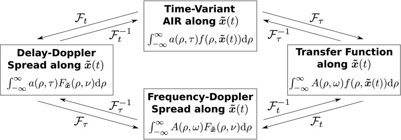
Figure 2. Representation of the four domains in Figure 1 subject to shaped parameters. The effective time-variance of the dynamic receiver channel is fully attributed to trajectory-shaped (filtered) versions of fixed sound-field parameters a(ρ, τ) and A(ρ, ω), respectively.

6.3 Sampled frequency spreading for periodic excitation

For obtaining a sampled analogy to (57), let us consider the periodic excitation

$s\left(n\right)=\tilde{s}\left(n\mathrm{mod}L\right)(58)$

by use of a deterministic sequence $\tilde{s}(n)$ of length L. In fact, this is the actual setting of various dynamic procedures that rely on the properties of so-called perfect sequences (Hahn and Spors, 2016; Katzberg et al., 2017b).

Based on (31), we define the short-time segment

$\begin{array}{cc}\hfill {\tilde{p}}_{\tilde{\mathit{x}}\left(n\right)}\left(w\right)& =\tilde{p}\left(\tilde{\mathit{x}}\left(n+w\right),n+w\right)\hfill \\ \hfill & ={\displaystyle \sum _{m=0}^{L-1}}s\left(n+w-m\right)h\left(\tilde{\mathit{x}}\left(n+w\right),m\right)\hfill \end{array}(59)$

of length L obtained from rectangular windowing of the microphone signal for window indices $w$ ∈ {0, …, L − 1}. Using (58), (59), the convolution theorem leads to

$\begin{array}{cc}\hfill {\tilde{p}}_{\tilde{\mathit{x}}\left(n\right)}\left(w\right)& =\frac{1}{L^2}{\displaystyle \sum _{m=0}^{L-1}}{\displaystyle \sum _{u=0}^{L-1}}{\displaystyle \sum _{l=0}^{L-1}}{\tilde{S}}_n\left(l\right){\mathrm{e}}^{-\mathrm{j}2\pi lm/L}{D}_{\tilde{\mathit{x}}\left(n\right)}\left(u-l,m\right){\mathrm{e}}^{\mathrm{j}2\pi uw/L}\hfill \\ \hfill & =\frac{1}{L^2}{\displaystyle \sum _{u=0}^{L-1}}{\displaystyle \sum _{l=0}^{L-1}}{\tilde{S}}_n\left(l\right)U_{\tilde{\mathit{x}}\left(n\right)}\left(u-l,l\right){\mathrm{e}}^{\mathrm{j}2\pi uw/L},\hfill \end{array}(60)$

with the discrete Fourier transform of the sequence $\tilde{s}(n)$ circularly shifted according to the excitation phase n mod L,

${\tilde{S}}_n\left(l\right)={\displaystyle \sum _{w=0}^{L-1}}\tilde{s}\left(w-n\mathrm{mod}L\right){\mathrm{e}}^{-\mathrm{j}2\pi lw/L},$

the (spatially) windowed Doppler-variant impulse response

$D_{\tilde{\mathit{x}}\left(n\right)}\left(u,m\right)={\displaystyle \sum _{w=0}^{L-1}}h\left(\tilde{\mathit{x}}\left(n+w\right),m\right){\mathrm{e}}^{-\mathrm{j}2\pi uw/L}$

shaped by the particular trajectory segment, and the corresponding transfer function

$U_{\tilde{\mathit{x}}\left(n\right)}\left(u,l\right)={\displaystyle \sum _{m=0}^{L-1}}{D}_{\tilde{\mathit{x}}\left(n\right)}\left(l,m\right){\mathrm{e}}^{-\mathrm{j}2\pi lm/L}$

modeling the frequency spread in the sampled signal due to the moving microphone. Taking the discrete Fourier transform of both sides of (60) yields

${\tilde{P}}_{\tilde{\mathit{x}}\left(n\right)}\left(u\right)=\frac{1}{L}{\displaystyle \sum _{l=0}^{L-1}}{\tilde{S}}_n\left(l\right)U_{\tilde{\mathit{x}}\left(n\right)}\left(u-l,l\right),(61)$

which clearly describes the resulting frequency shifts in the short-time Fourier representation ${\tilde{P}}_{\tilde{\mathit{x}}(n)}(u)$. The function ${\tilde{P}}_{\tilde{\mathit{x}}(n)}(u)$ displays the spatio-temporal spectrum measured under the positional variations along the particular trajectory segment.

6.4 Frequency-spreading filters due to moving microphones

The discrete spatialization model (29) allows for the sampled Doppler-variant representation

$\begin{array}{cc}\hfill U_{\tilde{\mathit{x}}\left(n\right)}\left(u,l\right)& ={\displaystyle \sum _{w=0}^{L-1}}H\left(\tilde{\mathit{x}}\left(n+w\right),l\right){\mathrm{e}}^{-\mathrm{j}2\pi uw/L}\hfill \\ \hfill & \approx {\displaystyle \sum _{c=0}^{C_l-1}}A\left(c,l\right)F_{\tilde{\mathit{x}}\left(n\right)}\left(c,u\right)\hfill \end{array}(62)$

subject to the finite set of sound-field parameters A(c, l) and the trajectory-dependent FIR filters

$F_{\tilde{\mathit{x}}\left(n\right)}\left(c,u\right)={\displaystyle \sum _{w=0}^{L-1}}f\left(c,\tilde{\mathit{x}}\left(n+w\right)\right){\mathrm{e}}^{-\mathrm{j}2\pi uw/L}(63)$

for the specific choice of spatial basis functions. Substituting (62) into (61) finally reveals the short-time Fourier representation

${\tilde{P}}_{\tilde{\mathit{x}}\left(n\right)}\left(u\right)=\frac{1}{L}{\displaystyle \sum _{l=0}^{L-1}}{\displaystyle \sum _{c=0}^{C_l-1}}{\tilde{S}}_n\left(l\right)A\left(c,l\right)F_{\tilde{\mathit{x}}\left(n\right)}\left(c,u-l\right)+N_{\tilde{\mathit{x}}\left(n\right)}\left(u\right)(64)$

of the dynamic sampling model (30) in terms of the frequency-spreading filters $F_{\tilde{\mathit{x}}(n)}(c,u)$, where $N_{\tilde{\mathit{x}}(n)}(u)$ encapsulates the frequency-dependent errors due to sampling and parameterization. At this, the particular Doppler spread is defined as the range of frequency bins over which $F_{\tilde{\mathit{x}}(n)}(c,u)$ is essentially non-zero. Note, for a non-moving microphone at constant position, i.e., $\tilde{\mathit{x}}(n)={\mathit{x}}_r$, the Doppler effect and the resulting frequency spreads vanish, which leads to inherent simplifications of (63), (64) according to

$F_{\tilde{\mathit{x}}\left(n\right)}\left(c,u\right)=Lf\left(c,{\mathit{x}}_r\right)\delta \left(u\right)$

and

${\tilde{P}}_{\tilde{\mathit{x}}\left(n\right)}\left(u\right)={\displaystyle \sum _{c=0}^{C_l-1}}{\tilde{S}}_n\left(u\right)A\left(c,u\right)f\left(c,{\mathit{x}}_r\right)+N_{\tilde{\mathit{x}}\left(n\right)}\left(u\right),(65)$

respectively, with (65) being actually dissolved into a short-time Fourier representation of the stationary sampling concept (4) for L-periodic excitation.

Similar to the subband procedure proposed in Section 5, the short-time Fourier analysis (64) could be used to set up a recovery strategy that decomposes the dynamic broadband problem (33) into multiple subproblems of narrow frequency ranges. In fact, this is straightforward for sufficiently slow trajectories which allow for approximations $F_{\tilde{\mathit{x}}(n)}(c,u)\approx Lf(c,\tilde{\mathit{x}}(n))\delta (u)$, i.e., the effect of spatio-spectral smearing is negligible within a time window of size L. However, having a microphone with arbitrary velocity profile, the modeling of decoupled sampling matrices from (64) with exact frequency-spreading filters $F_{\tilde{\mathit{x}}(n)}(c,u)$ and also the merging of obtained frequency estimates are not straightforward and clearly raise the complexity compared to the simple and universal subband procedure from Section 5, which requires only rough approximations of Doppler margins α_ℓ and β_ℓ.

7 Experiments and results

In this section, we demonstrate the key points of the introduced Doppler framework on the basis of experimental data and specifically chosen examples of parameterization models.

7.1 Doppler-spread visualizations

Let us first consider unrealistic toy examples with extreme receiver velocities for clear visualizations of both the Doppler shifts between dynamic subbands $H^{[\ell ]}(\tilde{\mathit{x}}(n),l)$ as elaborated in Section 5 and the Doppler-spreading FIR filters $F_{\tilde{\mathit{x}}(n)}(c,u)$ derived in Section 6. Using the image source method (Allen and Berkley, 1979), the sound field inside a room of size 5.80 m × 4.15 m × 2.55 m and reverberation time T₆₀ = 0.25 s was simulated. Instead of applying a nearest-neighbour interpolator as originally proposed by Allen and Berkley (1979), we took a Hanning-windowed ideal low-pass filter of length 4 ms to calculate the bandlimited and sampled RIR contributions from the particular image sources (Peterson, 1986). For the excitation sequence, we generated an L-periodic MLS signal (Rife and Vanderkooy, 1989) of about 20 s duration and filtered it in order to obtain a passband of effective audio frequencies between 400 Hz and 1600 Hz. We simulated corresponding (noiseless) audio recordings from an omnidirectional microphone sampling at f_s = 4000 Hz and continuously moving along Lissajous trajectories (Katzberg et al., 2017b). Lissajous curves for measurement are commonly used in magnetic particle imaging (Knopp et al., 2009). In (Katzberg et al., 2018), they have been experimentally shown to be a good choice also for sound-field sampling. The Lissajous trajectories considered here are typically slower and denser close to the volume boundaries, while the center regions are crossed fast and sampled more coarsely.

Four experiments were carried out with different trajectory mean velocities of 5 km/h, 50 km/h, 100 km/h, and 200 km/h. The spherical-harmonic parameterization from Section 3.3.2 was selected for the dynamic reconstruction. Accordingly, the spatially embedded transfer function sampled along ${\tilde{\mathit{x}}}_{◦}(n)$ is represented as

$H\left({\tilde{\mathit{x}}}_{◦}\left(n\right),l\right)\approx {\displaystyle \sum _{\left(v,q\right)\in {\mathrm{\Psi }}_l}}A\left(\left(v,q\right),l\right)b_v\left({\check{k}}_l{r}_n\right)Y_v^q\left({\theta }_n,{\varphi }_n\right),$

with ${\check{k}}_l={\omega }_l/c_0$ being the sampled angular wave number and Ψ_l constituting the set of index pairs where $v\le {\check{k}}_l{r}_{\text{max}}$ and |q| ≤ v (Rafaely, 2015). The radius of the target region was set to r_max = 0.1 m. The trajectory-dependent sampling of spatial basis functions reads $f(l,(v,q),{\tilde{\mathit{x}}}_{◦}(n))=b_v({\check{k}}_l{r}_n)Y_v^q({\theta }_n,{\varphi }_n)$. Using the analysis scheme from Section 5, we modeled $\mathcal{L}=5$ subband parameter vectors ${\mathit{a}}_{\ell }(\ell \in \{1,\dots ,\mathcal{L}\})$ with fullband margins, i.e., ${\mathcal{B}}_{\ell }=\{0,\dots ,L-1\}$ and ${\tilde{\mathbf{\Lambda }}}_{\ell }=\tilde{\mathbf{\Lambda }}$, and recovered them by solving the according overdetermined subproblems ${\tilde{\mathit{p}}}_{\ell }=\tilde{\mathbf{\Lambda }}{\mathit{a}}_{\ell }$ in the least-squares sense. For the chosen cutoffs ${\omega }_{\text{cut}}^{[\ell ]}=\ell 800\pi$, Hamming-windowed ideal band-pass filters of order 1000 were applied to the microphone signal. The frequency responses of these filters add up to unit magnitude with only minor variations in the order of 10^–4.

The absolute values of the recovered subband parameters A^[ℓ]((v, q), l) arranged in a_ℓ are depicted in Figure 3 in reference to the four numerical experiments with various microphone velocities. The parameters are successively concatenated first along the spatial (v, q)-dimensions and then along l with increasing frequency. Dotted lines indicate the vector indices where the defined cutoffs are reached. In Figure 3, the Doppler effect can be clearly observed in terms of subband-overlapping broadening of frequency-based parameters, especially with regard to higher frequencies and faster measurement trajectories. In case of 5 km/h, the subband of Doppler interfered frequencies in ${\tilde{\mathit{p}}}_{\ell }$ from the interval $\left[(\ell -1)400\mathrm{H}\mathrm{z},\ell 400\mathrm{H}\mathrm{z}\right]$ map to original frequencies in a_ℓ of nearly the same range when solving the modeled inverse problem. Here, the number of essential subband parameters may be vastly reduced in line with (47) using very tight Doppler margins. By contrast, considering the extremely high velocities, Doppler shifts induce a significant spreading of frequency information across multiple subbands and, thus, require large-scale margins. The parameter vector ${\mathit{a}}_5$, which refers to the highest frequency band, is basically inactive for low-speed trajectories. However, for velocities higher than 5 km/h, there are more and more signal contributions shifted to the higher frequencies of the subband sequence in ${\tilde{\mathit{p}}}_5$ (1600 Hz − 2000 Hz) and the corresponding subband parameter vector ${\mathit{a}}_5$ becomes increasingly essential for the sound-field recovery. On the left-hand side of Figure 3, the magnitudes of the broadband result a_full according to (33) without the subband decomposition are presented. They can be compared with the magnitudes of the cumulated subband vectors ${\displaystyle {\sum }_{\ell =1}^5}{\mathit{a}}_{\ell }$. Regardless of the trajectory speed, the recovered subband vectors effectively satisfy ${\displaystyle {\sum }_{\ell =1}^5}{\mathit{a}}_{\ell }={\mathit{a}}_{\text{full}}$ in each experiment, as expected according to (48). For each speed scenario, the deviation $\Vert {\mathit{a}}_{\text{full}}-{\displaystyle {\sum }_{\ell =1}^5}{\mathit{a}}_{\ell }{\Vert }_2^2/\Vert {\mathit{a}}_{\text{full}}{\Vert }_2^2$ is only about −35 dB.

Figure 3

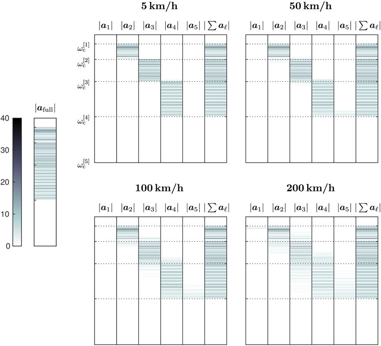
Figure 3. Magnitudes of spherical-harmonic parameters in vector |a_full| recovered from the broadband formulation in comparison to the magnitudes in |a_ℓ|, ℓ ∈ {1 …, 5}, recovered from the subband decomposition scheme for several trajectory velocities. Higher velocities induce a visible spreading of frequency information over different subbands.

By using the Doppler analysis scheme from Section 6, Figure 4 depicts several examples of the underlying frequency-spreading filters $F_{{\tilde{\mathit{x}}}_{◦}(n)}(l,(v,q),u)={\displaystyle {\sum }_{w=0}^{L-1}}f(l,(v,q),{\tilde{\mathit{x}}}_o(n+w)){\mathrm{e}}^{-\mathrm{j}2\pi uw/L}$. Here, the filter magnitudes |F₁(l, (v, q), u)| and |F₂(l, (v, q), u)| refer to particular trajectory segments in the 5 km/h and 50 km/h experiments, respectively, and the specific discrete frequencies l₁, l₂, l₃, and l₄ correspond to about 500 Hz, 1000 Hz, 1500 Hz, and 2000 Hz. In conformity with the entire model, the trajectory-dependent FIR filters show increased Doppler broadening for higher velocities and larger frequencies.

Figure 4

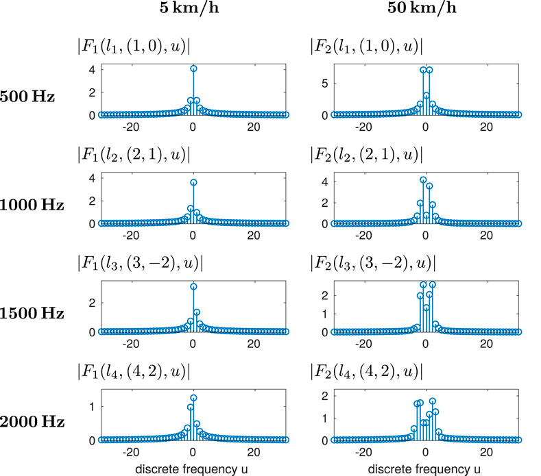
Figure 4. Lower- and higher-frequency examples (rows) of trajectory-dependent filters causing the Doppler spreading for two different trajectory velocities (columns). The range of the Doppler spread is defined by the effective filter length. It increases for higher frequencies and higher velocities.

7.2 Doppler misalignment due to noisy trajectory data

Inaccuracies in the positional tracking of the microphone result in Doppler-shift discrepancies as introduced in Section 4. The subband decoupling scheme from Section 5 may increase the robustness against noisy trajectory data, especially regarding low-frequency parameter estimates as highlighted in Section 5.4. For demonstrating such sensitivity relationships, we carried out numerical experiments in twenty simulated room scenarios, randomly chosen according the uniform distribution of box-shaped dimensions [2 m; 10 m]³ and reverberation times T₆₀ ∈ [0.2 s; 0.35 s]. In each environment, both the source position and the location of the considered measurement plane were randomly selected. Impulse responses were limited to length L = 4095. Recordings of an omnidirectional microphone were simulated at f_s = 12 kHz along planar Lissajous trajectories ${\tilde{\mathit{x}}}_{2\text{D}}(n)$ involving mean velocities of about 1 km/h. For the playback signal we used sixty repetitions of an L-periodic MLS. In several experiments, measurements were corrupted by additive white Gaussian noise with a signal-to-noise ratio (SNR) of 10 dB, 20 dB, and 30 dB, respectively. The underlying trajectory data were tested for the ideal case ${\tilde{\mathit{x}}}_{2\text{Dtrack}}(n)={\tilde{\mathit{x}}}_{2\text{D}}(n)$ and also for tracking errors according to ${\tilde{\mathit{x}}}_{2\text{Dtrack}}(n)={\tilde{\mathit{x}}}_{2\text{D}}(n)+{\stackrel{*}{\mathit{x}}}_{2\text{D}}(n)$, with positional noise ${\stackrel{*}{\mathit{x}}}_{2\text{D}}(n)$ independently drawn from the zero-mean normal distribution with standard deviation σ_ξ for each of the effective dimensions ξ ∈ {x, y}. The mismatch level was set to σ_ξ = 3 mm and σ_ξ = 6 mm, respectively.

The grid approach from Section 3.3.3 was combined with aspects from theoretical acoustics and used for CS-based sound-field recovery (Katzberg et al., 2018; Katzberg and Mertins, 2022). Regarding the experiments with two-dimensional trajectories on planar target regions, the discretized sound-field model on a finite G_x × G_y grid reads

$H\left({\tilde{\mathit{x}}}_{2\text{D}}\left(n\right),l\right)\approx {\displaystyle \sum _{\left({\kappa }_x,{\kappa }_y\right)\in {\mathrm{\Gamma }}_l}}{\mathcal{H}}_{\text{s}}\left({\left[{\kappa }_x,{\kappa }_y\right]}^T,l\right){\mathrm{e}}^{\mathrm{j}2\pi {\tilde{g}}_x\left(n\right){\kappa }_x/G_x}{\mathrm{e}}^{\mathrm{j}2\pi {\tilde{g}}_y\left(n\right){\kappa }_y/G_y},$

where ${\tilde{g}}_x(n)=(\tilde{x}(n)-{\mu }_x)/{\mathrm{\Delta }}_x$ and ${\tilde{g}}_y(n)=(\tilde{y}(n)-{\mu }_y)/{\mathrm{\Delta }}_y$ are the grid-related trajectory coordinates subject to the selected grid origin μ_ξ and spacing Δ_ξ for ξ ∈ {x, y}, κ_ξ denotes the integer-valued frequency indices that translate to sampled spatial frequencies according to $k_{{\kappa }_{\xi }}=2\pi {\mathrm{\Delta }}_{\xi }^{-1}{\kappa }_{\xi }/G_{\xi }$, and Γ_l represents the set of discrete frequency pairs (κ_x, κ_y) that approximate the conical structure around the sampled temporal frequency ω_l = 2πf_sl/L (Katzberg et al., 2018; Katzberg and Mertins, 2022). Complying with the proposed Doppler framework, the trajectory-dependent sampling of associated basis functions in space reads $f(({\kappa }_x,{\kappa }_y),{\tilde{\mathit{x}}}_{2\text{D}}(n))={\mathrm{e}}^{\mathrm{j}2\pi {\tilde{g}}_x(n){\kappa }_x/G_x}{\mathrm{e}}^{\mathrm{j}2\pi {\tilde{g}}_y(n){\kappa }_y/G_y}$. The following recovery results were obtained with a grid design of G_x = G_y = 25 and Δ_x = Δ_y = 0.019 m.

As error measure for the overall sound-field reconstruction involving G grid AIRs, the mean normalized system misalignment $\text{MNSM}=1/G{\displaystyle {\sum }_{g=1}^G}\Vert {\mathit{h}}_g-{\widehat{\mathit{h}}}_g{\Vert }_2^2/\Vert {\mathit{h}}_g{\Vert }_2^2$ is used, with ${\mathit{h}}_g\in {\mathbb{R}}^L$ containing the true AIR and ${\widehat{\mathit{h}}}_g\in {\mathbb{R}}^L$ being the recovered AIR at grid index $g$. The results for the broadband model according to Section 3 and for the subband decomposition scheme according to Section 5 are comparatively depicted in Figure 5 subject to the different levels of trajectory noise. The outcomes over all experimental room scenarios are presented by use of boxplots. For the subband strategy, Hamming-windowed ideal band-pass filters of order 5000 were applied, summing up to unit magnitude response with slight errors of order 10^–5. We chose $\mathcal{L}=6$, ${\omega }_{\text{cut}}^{[\ell ]}=\ell 2000\pi$, and Doppler margins α_ℓ, β_ℓ that cover about twenty discrete frequency bins each. This decomposes the primary problem subject to $\tilde{\mathbf{\Lambda }}\in {\mathbb{C}}^{M\times P}$ into six decoupled subproblems subject to ${\tilde{\mathbf{\Lambda }}}_{\ell }\in {\mathbb{C}}^{M\times P_{\ell }}$ referring to successive 1 kHz frequency ranges. The corresponding numbers P and P_ℓ of spatio-temporal parameters are listed in Table 1. Besides, there are the respective values of the perturbation measure $\Vert \stackrel{*}{\mathit{E}}{\Vert }_{\text{F}}$ from Section 4 for rating the induced Doppler-shift mismatches due to the tested positional noise.

Figure 5

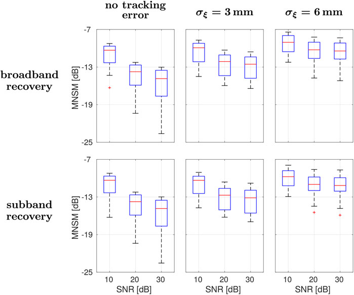
Figure 5. Errors of AIR parameters obtained from the broadband (first row) and subband formulations (second row) for various microphone SNRs and different levels of tracking inaccuracies (columns).

Table 1

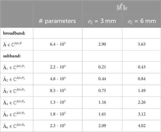
Table 1. Comparison of parameter numbers for the broadband and subband strategies, and evaluation of matrix perturbations due to positional deviations of σ_ξ = 3 mm and σ_ξ = 6 mm, respectively.

While the recovery performances are essentially equal for noiseless trajectory data, the subband scheme improves the robustness against the trajectory discrepancies compared to the standard broadband approach. For σ_ξ = 6 mm, its performance gain is about 1 dB on average (Figure 5). For visualizing the effects of positional inaccuracies, the magnitudes of two particular frequency-spreading filters F₁((κ_x, κ_y), u) are presented in Figure 6 given a true trajectory segment and its noisy version: for filters such as F₁((10, 10), u) pointing to rather higher spatial frequencies (and, thus, also to higher temporal frequencies), the resulting Doppler mismatches are typically more considerable. To analyze frequency-based recovery performances, we apply the mean energy spectral density of the error $\text{FRQ}-\text{ERR}(f)=1/G{\displaystyle {\sum }_{g=1}^G}|H_g(f)-{\widehat{H}}_g(f){|}^2$, where $H_g$(f) and ${\widehat{H}}_g(f)$ are the Fourier transforms of the true and estimated grid AIRs, respectively. The frequency errors of the broadband and subband procedures for σ_ξ = 6 mm are presented in Figure 7. In line with the considerations made in Section 5.4, the benefit of the subband strategy is especially apparent in the lower halfband up to 3 kHz, where the inverse problem is modeled by the smaller-sized sampling matrices ${\tilde{\mathbf{\Lambda }}}_1$, ${\tilde{\mathbf{\Lambda }}}_2$, and ${\tilde{\mathbf{\Lambda }}}_3$ (cf. Table 1).

Figure 6

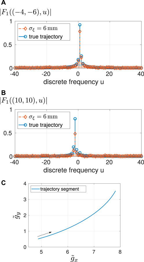
Figure 6. Outline of mismatched and true Doppler-spreading filters F₁((κ_x, κ_y), u) for discrete-frequency pairs of (A) (κ_x, κ_y) = (−4, − 6) and (B) (κ_x, κ_y) = (10, 10). The underlying true trajectory segment is depicted in (C), where the arrow indicates the direction of microphone motion. Note that there is an intuitive filter interpretation due to the applied uniform-grid model (cf. Section 3.3.3). For example, F₁((10,10), u) can be considered to render the trajectory-dependent Doppler effect for a virtual plane wave arriving from direction [−1, − 1], i.e., it basically shifts the sound-field parameters to lower frequencies as can be seen from (B).

Figure 7

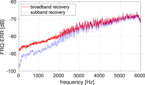
Figure 7. Frequency-dependent errors of recovered sound-field parameters. The subband approach allows for improved reconstructions especially at low frequencies.

8 Conclusion

In this work, we formulated a Doppler-based framework that reveals the frequency-spreading effects in dynamic sound-field sampling procedures. It has been shown that the exact positional tracking of a moving microphone allows for the exact rendering of underlying Doppler shifts in the acquired signal. As it turned out, the involved frequency shifts are directly connected with the sampling of spatial basis functions subject to the microphone trajectory. For the practically relevant case of tracking inaccuracies, we described the resulting impact on the inverse problem in terms of mismatches between true and inaccurately modeled Doppler shifts. Such mismatches lead to a multiplicative perturbation model, for which we provided sensitivity considerations regarding least-squares and CS-based estimates. Also, a subband analysis scheme has been derived, which enables us to split the presented Doppler model for broadband measurements into a number of smaller subproblems that consider particular frequency bands. This allows for parallelizing the computational effort and for obtaining faster reconstructions with improved robustness against the trajectory errors, especially regarding lower frequencies. Further, we provided a reasonable concept for the (short-time) Fourier analysis of the dynamic measurement signal. Due to the continuously moving microphone, this yields an actually spatio-temporal Fourier description, dimensionally coupled by the performed trajectory. In this representation, the included Doppler spreads can be explicitly characterized by a series of trajectory-dependent FIR filters.

Data availability statement

The original contributions presented in the study are included in the article/supplementary material, further inquiries can be directed to the corresponding author.

Author contributions

FK: Writing–original draft. MM: Writing–review and editing. AM: Writing–review and editing.

Funding

The author(s) declare financial support was received for the research, authorship, and/or publication of this article. This work has been supported in part by the German Research Foundation under Grant No. ME 1170/10-2.

Conflict of interest

The authors declare that the research was conducted in the absence of any commercial or financial relationships that could be construed as a potential conflict of interest.

Publisher’s note

All claims expressed in this article are solely those of the authors and do not necessarily represent those of their affiliated organizations, or those of the publisher, the editors and the reviewers. Any product that may be evaluated in this article, or claim that may be made by its manufacturer, is not guaranteed or endorsed by the publisher.

References

Ajdler, T., Sbaiz, L., and Vetterli, M. (2006). The plenacoustic function and its sampling. IEEE Trans. Signal Process. 54, 3790–3804. doi:10.1109/tsp.2006.879280

CrossRef Full Text | Google Scholar

Ajdler, T., Sbaiz, L., and Vetterli, M. (2007). Dynamic measurement of room impulse responses using a moving microphone. J. Acoust. Soc. Am. 122, 1636–1645. doi:10.1121/1.2766776

PubMed Abstract | CrossRef Full Text | Google Scholar

Allen, J., and Berkley, D. (1979). Image method for efficiently simulating small-room acoustics. J. Acoust. Soc. Am. 65, 943–950. doi:10.1121/1.382599

CrossRef Full Text | Google Scholar

Bah, B., and Tanner, J. (2010). Improved bounds on restricted isometry constants for Gaussian matrices. SIAM J. Matrix Anal. Appl. 31, 2882–2898. doi:10.1137/100788884

CrossRef Full Text | Google Scholar

Bello, P. (1963). Characterization of randomly time-variant linear channels. IEEE Trans. Commun. Syst. 11, 360–393. doi:10.1109/tcom.1963.1088793

CrossRef Full Text | Google Scholar

Benesty, J., Huang, Y., Chen, J., and Naylor, P. A. (2006). “Adaptive algorithms for the identification of sparse impulse responses,” in Topics in acoustic echo and noise control. Editors E. Hänsler, and G. Schmidt (Berlin: Springer), 125–153.

Google Scholar

J. Benesty, M. Sondhi, and Y. Huang (2008). Springer handbook of speech processing (Germany: Springer).

Google Scholar

Björck, Å. (1996). Numerical methods for least squares problems (SIAM) United States: SIAM.

Google Scholar

Candès, E., Romberg, J., and Tao, T. (2006). Stable signal recovery from incomplete and inaccurate measurements. Commun. Pure Appl. Math. 59, 1207–1223. doi:10.1002/cpa.20124

CrossRef Full Text | Google Scholar

Colton, D., and Kress, R. (2019). Inverse acoustic and electromagnetic scattering theory. 4 edn. Germany: Springer.

Google Scholar

Enzner, G. (2008). Analysis and optimal control of LMS-type adaptive filtering for continuous-azimuth acquisition of head related impulse responses. Proc. IEEE Int. Conf. Acoust. Speech, Signal Process., 393–396. doi:10.1109/ICASSP.2008.4517629

CrossRef Full Text | Google Scholar

Fazi, F. M., Noisternig, M., and Warusfel, O. (2012). Representation of sound fields for audio recording and reproduction. Proc. Acoust., 859–865.

Google Scholar

Golub, G. H., and Van Loan, C. F. (2013). Matrix computations. 4 edn. United States: Johns Hopkins University Press.

Google Scholar

Grami, A. (2016). Introduction to digital communications. United States: Academic Press.

Google Scholar

Hahn, N., Hahne, W., and Spors, S. (2017). Dynamic measurement of binaural room impulse responses using an optical tracking system. Proc. Int. Conf. Spat. Audio., 16–21. doi:10.1109/WASPAA.2017.81700241

CrossRef Full Text | Google Scholar

Hahn, N., and Spors, S. (2016). Comparison of continuous measurement techniques for spatial room impulse responses. Proc. Eur. Signal Process. Conf., 1638–1642. doi:10.1109/EUSIPCO.2016.7760526

CrossRef Full Text | Google Scholar

Hahn, N., and Spors, S. (2017). Continuous measurement of spatial room impulse responses using a non-uniformly moving microphone. IEEE Workshop Appl. Signal Process. Audio Acoust, 205–208.

CrossRef Full Text | Google Scholar

Hahn, N., and Spors, S. (2018). Simultaneous measurement of spatial room impulse responses from multiple sound sources using a continuously moving microphone. Proc. Eur. Signal Process. Conf., 2194–2198. doi:10.23919/EUSIPCO.2018.8553532

CrossRef Full Text | Google Scholar

Haykin, S. (2001). Adaptive filter theory. USA: Prentice Hall.

Google Scholar

S. Haykin, and K. J. R. Liu (2010). Handbook on array processing and sensor networks (New York: Wiley).

Google Scholar

He, J., Ranjan, R., Gan, W.-S., Chaudhary, N. K., Hai, N. D., and Gupta, R. (2018). Fast continuous measurement of HRTFs with unconstrained head movements for 3D audio. J. Audio Eng. Soc. 66, 884–900. doi:10.17743/jaes.2018.0050

CrossRef Full Text | Google Scholar

Herman, M., and Strohmer, T. (2010). General deviants: an analysis of perturbations in compressed sensing. IEEE J. Sel. Top. Signal Process. 4, 342–349. doi:10.1109/jstsp.2009.2039170

CrossRef Full Text | Google Scholar

Higham, N. J. (2002). Accuracy and stability of numerical algorithms. United States: SIAM.

Google Scholar

F. Hlawatsch, and G. Matz (2011). Wireless communications over rapidly time-varying channels (USA: Academic Press).

Google Scholar

Katzberg, F., Maass, M., and Mertins, A. (2021). Spherical harmonic representation for dynamic sound-field measurements. Proc. IEEE Int. Conf. Acoust. Speech, Signal Process., 426–430. doi:10.1109/ICASSP39728.2021.9413708

CrossRef Full Text | Google Scholar

Katzberg, F., Maass, M., Pallenberg, R., and Mertins, A. (2022). Positional tracking of a moving microphone in reverberant scenes by applying perfect sequences to distributed loudspeakers. Proc. Int. Workshop Acoust. Signal Enhanc. doi:10.1109/IWAENC53105.2022.9914709

CrossRef Full Text | Google Scholar

Katzberg, F., Mazur, R., Maass, M., Koch, P., and Mertins, A. (2017a). Multigrid reconstruction of sound fields using moving microphones. Proc. Workshop Hands-free Speech Commun. Microphone Arrays, 191–195. doi:10.1109/HSCMA.2017.7895588

CrossRef Full Text | Google Scholar

Katzberg, F., Mazur, R., Maass, M., Koch, P., and Mertins, A. (2017b). Sound-field measurement with moving microphones. J. Acoust. Soc. Am. 141, 3220–3235. doi:10.1121/1.4983093

PubMed Abstract | CrossRef Full Text | Google Scholar

Katzberg, F., Mazur, R., Maass, M., Koch, P., and Mertins, A. (2018). A compressed sensing framework for dynamic sound-field measurements. IEEE/ACM Trans. Audio, Speech, Lang. Process. 26, 1962–1975. doi:10.1109/taslp.2018.2851144

CrossRef Full Text | Google Scholar

Katzberg, F., and Mertins, A. (2022). “Sparse recovery of sound fields using measurements from moving microphones,” in Compressed sensing in information processing. Editors G. Kutyniok, H. Rauhut, and R. J. Kunsch (Germany: Springer), 377–411.

CrossRef Full Text | Google Scholar

Knopp, T., Biederer, S., Sattel, T., Weizenecker, J., Gleich, B., Borgert, J., et al. (2009). Trajectory analysis for magnetic particle imaging. Phys. Med. Biol. 54, 385–397. doi:10.1088/0031-9155/54/2/014

PubMed Abstract | CrossRef Full Text | Google Scholar

Li, W., and Preisig, J. C. (2007). Estimation of rapidly time-varying sparse channels. IEEE J. Ocean. Eng. 32, 927–939. doi:10.1109/joe.2007.906409

CrossRef Full Text | Google Scholar

Moreau, S., Daniel, J., and Bertet, S. (2006). 3D sound field recording with higher order ambisonics - objective measurements and validation of a 4th order spherical microphone. Proc. 120th Conv. Audio Eng. Soc. (Conv. Paper 6857).

Google Scholar

Morse, P. M., and Ingard, K. U. (1986). Theoretical acoustics. USA: Princeton University Press.

Google Scholar

Ostashev, V. E., and Wilson, D. K. (2019). Acoustics in moving inhomogeneous media. 2 edn. United States: CRC Press.

Google Scholar

Peterson, P. M. (1986). Simulating the response of multiple microphones to a single acoustic source in a reverberant room. J. Acoust. Soc. Am. 80, 1527–1529. doi:10.1121/1.394357

PubMed Abstract | CrossRef Full Text | Google Scholar

Pierce, A. D. (2019). Acoustics: an introduction to its physical principles and applications. Germany: Springer.

Google Scholar

Rafaely, B. (2005). Analysis and design of spherical microphone arrays. IEEE Trans. Speech Audio Process 12, 135–143. doi:10.1109/tsa.2004.839244

CrossRef Full Text | Google Scholar

Rafaely, B. (2015). Fundamentals of spherical array processing. Germany: Springer.

Google Scholar

Rife, D. D., and Vanderkooy, J. (1989). Transfer-function measurement with maximum-length sequences. J. Audio Eng. Soc. 37, 419–444.

Google Scholar

Sondhi, M. (1967). An adaptive echo canceller. Bell Syst. Tech. J. 46, 497–511. doi:10.1002/j.1538-7305.1967.tb04231.x

CrossRef Full Text | Google Scholar

Stan, G.-B., Embrechts, J.-J., and Archambeau, D. (2002). Comparison of different impulse response measurement techniques. J. Audio Eng. Soc. 50, 249–262.

Google Scholar

Stewart, G. W. (1977). On the perturbation of pseudo-inverses, projections and linear least squares problems. SIAM Rev. 19, 634–662. doi:10.1137/1019104

CrossRef Full Text | Google Scholar

Thompson, R. C. (1972). Principal submatrices IX: interlacing inequalities for singular values of submatrices. Linear Algebra Appl. 5, 1–12. doi:10.1016/0024-3795(72)90013-4

CrossRef Full Text | Google Scholar

Urbanietz, C., and Enzner, G. (2020). Direct spatial-Fourier regression of HRIRs from multi-elevation continuous-azimuth recordings. IEEE/ACM Trans. Audio, Speech, Lang. Process. 28, 1129–1142. doi:10.1109/taslp.2020.2982291

CrossRef Full Text | Google Scholar

Välimäki, V., and Laakso, T. (2000). Principles of fractional delay filters. Proc. IEEE Int. Conf. Acoust. Speech, Signal Process., 3870–3873. doi:10.1109/ICASSP.2000.860248

CrossRef Full Text | Google Scholar

Vasquez, F. G., and Mauck, C. (2018). Approximation by Herglotz wave functions. SIAM J. Appl. Math. 78, 1283–1299. doi:10.1137/17m1144234

CrossRef Full Text | Google Scholar

Wedin, P.-Å. (1973). Perturbation theory for pseudo-inverses. BIT Numer. Math. 13, 217–232. doi:10.1007/bf01933494

CrossRef Full Text | Google Scholar

Williams, E. G. (1999). Fourier acoustics – sound radiation and nearfield acoustical holography. United States: Academic Press.

Google Scholar

Zeng, W.-J., and Xu, W. (2012). Fast estimation of sparse doubly spread acoustic channels. J. Acoust. Soc. Am. 131, 303–317. doi:10.1121/1.3665992

PubMed Abstract | CrossRef Full Text | Google Scholar