Optimized quantization parameter selection for video-based point cloud compression

Point clouds are sets of points used to visualize three-dimensional (3D) objects. Point clouds can be static or dynamic. Each point is characterized by its 3D geometry coordinates and attributes such as color. High-quality visualizations often require millions of points, resulting in large storage and transmission costs, especially for dynamic point clouds. To address this problem, the moving picture experts group has recently developed a compression standard for dynamic point clouds called video-based point cloud compression (V-PCC). The standard generates two-dimensional videos from the geometry and color information of the point cloud sequence. Each video is then compressed with a video coder, which converts each frame into frequency coefficients and quantizes them using a quantization parameter (QP). Traditionally, the QPs are severely constrained. For example, in the low-delay configuration of the V-PCC reference software, the quantization parameter values of all the frames in a group of pictures are set to be equal. We show that the rate-distortion performance can be improved by relaxing this constraint and treating the QP selection problem as a multi-variable constrained combinatorial optimization problem, where the variables are the QPs. To solve the optimization problem, we propose a variant of the differential evolution (DE) algorithm. Differential evolution is an evolutionary algorithm that has been successfully applied to various optimization problems. In DE, an initial population of randomly generated candidate solutions is iteratively improved. At each iteration, mutants are generated from the population. Crossover between a mutant and a parent produces offspring. If the performance of the offspring is better than that of the parent, the offspring replaces the parent. While DE was initially introduced for continuous unconstrained optimization problems, we adapt it for our constrained combinatorial optimization problem. Also, unlike standard DE, we apply individual mutation to each variable. Furthermore, we use a variable crossover rate to balance exploration and exploitation. Experimental results for the low-delay configuration of the V-PCC reference software show that our method can reduce the average bitrate by up to 43% compared to a method that uses the same QP values for all frames and selects them according to an interior point method.

1 Introduction

Extensive research has been conducted to create effective representations for 3D content. Among these representations, point clouds are gaining increasing popularity due to their ability to support computer vision tasks and immersive experience applications such as virtual reality and augmented reality.

A point cloud is a set of points lying on the surface of a 3D content. Each point of a point cloud is given by its 3D coordinates and a number of attributes such as color, reflectance, or surface normal. Point clouds can be generated with 3D scanners or photogrammetry software. Modern point cloud processing software use computer graphics algorithms such as marching cubes to reconstruct the surface of the content from the point cloud Berger et al. (2017).

Since point clouds typically consist of millions of points, efficient compression techniques are required to reduce storage and bandwidth costs. The most popular point cloud compression techniques are the two standards developed by the moving picture experts group (MPEG) Graziosi et al. (2020): geometry-based point cloud compression (G-PCC) and video-based point cloud compression (V-PCC). In this paper, we focus on V-PCC ISO/IEC (2020a), which provides competitive compression results for both static and dynamic point clouds Wu et al. (2022).

Figure 1 shows the architecture of the V-PCC encoder. For each point cloud (frame) in a sequence of point clouds, three two-dimensional (2D) images are generated: one image that corresponds to the geometry information, one image that corresponds to the color information, and one binary image called occupancy map used to decide whether a 3D point should be reconstructed (Figure 2). Next, the geometry video and color video are compressed with a lossy video coder, e.g., H.265/HEVC Sullivan et al. (2012), while the occupancy video is usually compressed with a lossless video coder. A critical step in the compression of the geometry video and color video is quantization, which is controlled by a quantization parameter (QP) or, equivalently, a quantization step size Qstep. In video coding, pixel values from a given frame are predicted using encoded information from the same frame (intra-prediction) or from other frames (inter-prediction). Subsequently, transforms are applied to the residual blocks derived from these predictions. The resulting transform coefficients are then quantized by dividing them by a quantization step size and rounding off the results to obtain quantized coefficients. When HEVC is used, the available QP values are the 52 integers 0,1, ..., 51. An approximate relationship between the QP value and the quantization step size is $Qstep=2^{\frac{QP-4}{6}}$ Budagavi et al. (2014). Higher QP values reduce the bitrate but increase the reconstruction error (distortion).

Figure 1

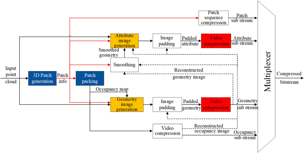
Figure 1. V-PCC encoder ISO/IEC (2020a).

Figure 2

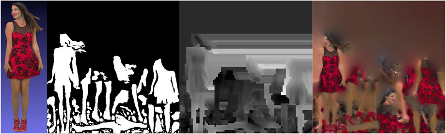
Figure 2. From left to right: original point cloud, occupancy map, geometry image, and color image.

One fundamental problem is the selection of the QP values that minimize the overall distortion given a target bit budget. In the reference software (test model) ISO/IEC (2020b) of the V-PCC standard, this problem is not addressed. For example, for the low-delay configuration of the software, it is assumed that the QP values of all the frames in a group of frames are equal.

Our paper addresses this fundamental problem in two ways. First, we formulate the QP selection problem as a constrained combinatorial optimization problem where the variables are the QP values of the frames. Second, we propose a novel implementation of the differential evolution (DE) algorithm Price et al. (2005) to solve the problem. DE is a popular metaheuristic, which has demonstrated excellent performance on many global optimization problems Das and Suganthan (2011); Xue et al. (2022). Compared to other evolutionary algorithms, it is easier to implement and requires fewer parameters to adjust (only three). While DE was initially introduced for continuous unconstrained optimization problems, we adapt it to our combinatorial constrained optimization problem.

The remainder of the paper is organized as follows. In Section 2, we formulate the constrained combinatorial optimization problem that we aim to solve. In Section 3, we discuss related work. In Section 4, we outline the variant of DE proposed in this paper to select the quantization parameters. In Section 5, we compare the performance of the proposed method to that of the state-of-the-art Liu et al. (2021). In Section 6, we give concluding comments and suggest future work. This paper is an extended version of our conference paper Yuan et al. (2021d). We expand the literature review, provide a more detailed analysis of our method, give visual quality results, show how the QP selection problem can be tackled when the point cloud comprises multiple groups of frames, and extend our optimization framework to accommodate variable QP values within a frame.

2 Problem formulation

Suppose that we are given a sequence of N point clouds (frames) and a bit budget R_T. Our aim is to select for each frame i(i = 1, …, N), the quantization step size Q_g,i for the geometry video and the quantization step size Q_c,i for the color video in an optimal way. Both Q_g,i and Q_c,i are to be selected from the same finite set $\mathcal{S}=\{q_0,\dots ,q_{M-1}\}$. We formulate this problem as the constrained multi-objective optimization problem

$\begin{array}{c}\hfill \underset{{\mathbf{Q}}_{\mathbf{g}},{\mathbf{Q}}_{\mathbf{c}}}{\min }\left[D_g\left({\mathbf{Q}}_{\mathbf{g}},{\mathbf{Q}}_{\mathbf{c}}\right),D_c\left({\mathbf{Q}}_{\mathbf{g}},{\mathbf{Q}}_{\mathbf{c}}\right)\right]\\ \hfill \text{subject\hspace{0.17em}to\hspace{0.17em}}R\left({\mathbf{Q}}_{\mathbf{g}},{\mathbf{Q}}_{\mathbf{c}}\right)\le R_T\end{array}(1)$

where Q_g = (Q_g,1, Q_g,2, …, Q_g,N), Q_c = (Q_c,1, Q_c,2, …, Q_c,N), D_g(Q_g, Q_c) is the geometry distortion (error between the 3D coordinates of the points in the original point cloud and the 3D coordinates of the points in the point cloud obtained after reconstructing the point cloud from its compressed version), D_c(Q_g, Q_c) is the color distortion (error between the color of the points in the original point cloud and the color of the points in the point cloud obtained after reconstructing the point cloud from its compressed version), and R(Q_g, Q_c) is the number of bits allocated to the geometry and color information in the compressed point cloud. Here,

$D_g\left({\mathbf{Q}}_{\mathbf{g}},{\mathbf{Q}}_{\mathbf{c}}\right)=\frac{1}{N}{\displaystyle \sum _{i=1}^N}{D}_{g,i}\left(Q_{g,i},Q_{c,i}\right),(2)$

$D_c\left({\mathbf{Q}}_{\mathbf{g}},{\mathbf{Q}}_{\mathbf{c}}\right)=\frac{1}{N}{\displaystyle \sum _{i=1}^N}{D}_{c,i}\left(Q_{g,i},Q_{c,i}\right),(3)$

where D_g,i(Q_g,i, Q_c,i) and D_c,i(Q_g,i, Q_c,i) are the geometry and color distortions of the ith frame, respectively. Similarly,

$R\left({\mathbf{Q}}_{\mathbf{g}},{\mathbf{Q}}_{\mathbf{c}}\right)={\displaystyle \sum _{i=1}^N}{R}_{g,i}\left(Q_{g,i},Q_{c,i}\right)+R_{c,i}\left(Q_{g,i},Q_{c,i}\right),(4)$

where R_g,i(Q_g,i, Q_c,i) and R_c,i(Q_g,i, Q_c,i) are the number of bits for the geometry and color information in the ith frame, respectively.

Since the functions D_g and R_g,i do not depend on the colour quantization parameters, the terms D_g(Q_g, Q_c) and R_g,i(Q_g,i, Q_c,i) can be simplified to D_g(Q_g) and R_g,i(Q_g,i).

To simplify problem (1), we scalarize it as

$\begin{array}{c}\hfill \underset{{\mathbf{Q}}_{\mathbf{g}},{\mathbf{Q}}_{\mathbf{c}}}{\min }\omega D_g\left({\mathbf{Q}}_{\mathbf{g}},{\mathbf{Q}}_{\mathbf{c}}\right)+\left(1-\omega \right)D_c\left({\mathbf{Q}}_{\mathbf{g}},{\mathbf{Q}}_{\mathbf{c}}\right)\\ \hfill \text{subject\hspace{0.17em}to\hspace{0.17em}}R\left({\mathbf{Q}}_{\mathbf{g}},{\mathbf{Q}}_{\mathbf{c}}\right)\le R_T\end{array}(5)$

where ω is a weighting factor that trades off the geometry distortion against the color distortion. As the number of candidates in the problem is M^2N, finding an optimal solution with exhaustive search is not feasible when either M or N is large. This is the case in V-PCC, where M = 52 when HEVC is used, and N is typically at least equal to 4.

3 Related work

Extensive research has been conducted on finding globally optimal QPs for a group of frames in a 2D video. Ramchandran et al. (1994) propose a tree-based algorithm to obtain an optimal solution by assuming a monotonicity condition. However, the high time complexity of the algorithm renders it impractical Fiengo et al. (2017). Huang and Hang (2009) add a constraint on permissible video quality fluctuation across the frames and use the Viterbi algorithm to compute an optimal solution. To reduce the time complexity of the algorithm, the authors make assumptions of monotonicity and node clustering, which are not always valid. Fiengo et al. (2017) develop an analytical convex rate-distortion model for HEVC that accounts for inter-frame dependencies. The model uses a primal-dual algorithm to compute the optimal rate for each frame. However, since an approximation of the rate-distortion function is used, the solution may not be globally optimal. Moreover, the algorithm treats the problem as continuous, while the QP values are finite. Another approach, known as quantization parameter cascading, allocates different QP values to frames based on their hierarchical layer within a group of pictures Li et al. (2010), McCann et al. (2014), Zhao et al. (2016), Marzuki and Sim (2020). This approach is based on the observation that frames in lower layers contribute more to the overall rate-distortion performance than those in higher layers. However, this approach is applicable only to hierarchical prediction structures. HoangVan et al. (2021) use a trellis-based algorithm to adaptively select the QP value for each coded picture in a group of pictures. However, the algorithm is not guaranteed to find an optimal solution as it uses a greedy search strategy. Moreover, to reduce the complexity of the algorithm, both the number of candidate QP values and the number of iterations in the algorithm are severely constrained.

There is a lack of research on optimal QP selection for V-PCC. Extending the methods proposed for 2D video to V-PCC is challenging because the QP values have to be selected for two videos simultaneously. In the MPEG V-PCC test model ISO/IEC (2020b), the QP values are not optimized. For a given group of frames, one selects the QP values for the first frame, and the QP values for subsequent frames within the same group are set based on a fixed difference (e.g., zero, which is the default value in the low-delay configuration). This approach presents two major limitations: First, when aiming for a specific bitrate, there is no defined method for selecting the QP values for the first frame. Second, the enforced relationship between the QP values of the first frame and those of the following frames can compromise the rate-distortion performance.

In Liu et al. (2021), mathematical models for the rate and distortion are obtained via statistical analysis. The work assumes that QP_g,i = QP_g,1 and QP_c,i = QP_c,1 for i = 2, …, N, where QP_g,i and QP_c,i are the geometry QP and color QP values for the ith frame in a group of N frames, respectively. More precisely, the geometry distortion D_g is modeled as α_gQ_g,1 + β_g, the color distortion D_c is modeled as α_gcQ_g,1 + α_ccQ_c,1 + β_c, the number of bits for the geometry information is modeled as ${\gamma }_g{Q}_{g,1}^{{\theta }_g}$, and the number of bits for the color information is modeled as ${\gamma }_c{Q}_{c,1}^{{\theta }_c}$, where α_g, β_g, α_gc, α_cc, β_c, γ_g, θ_g, γ_c, θ_c are parameters for the models. Then, problem (5) is written as

$\begin{array}{c}\hfill \underset{Q_{g,1},Q_{c,1}}{\min }a{Q}_{g,1}+b{Q}_{c,1}+c\\ \hfill \text{subject\hspace{0.17em}to\hspace{0.17em}}{\gamma }_g{Q}_{g,1}^{{\theta }_g}+{\gamma }_c{Q}_{c,1}^{{\theta }_c}\le R_T\end{array}(6)$

where a, b, and c are parameters, and solved using an interior point method. Experimental results indicate that the method achieves comparable rate-distortion performance to exhaustive search (with the same constraint on the QP values) but with significantly lower time complexity. In Liu et al. (2020), the authors use the approach introduced in Liu et al. (2021) to allocate the total bitrate between the geometry and color information. They further partition each frame into seven regions and derive analytical models for the rate and distortion of each region. Subsequently, the optimal geometry QP values for all regions are obtained by minimizing the total geometry distortion subject to the allocated geometry bitrate. Finally, the optimal color QP values for the regions are determined by minimizing the total color distortion subject to the allocated color bitrate based on the optimal geometry QP values. Results for static point clouds show better rate accuracy but lower rate-distortion performance than the method in Liu et al. (2021). Although both methods are computationally efficient, their rate-distortion performance is restricted by the equality constraint on the QP values.

In Yuan et al. (2021a), the equality constraint on the QP values is lifted, and the QP selection problem is formulated as in (5). In addition, analytical models for the distortion and color functions are introduced. The distortion model of frame i is given as

$\begin{array}{cc}\hfill D_{g,i}& ={\alpha }_{g,i}{Q}_{g,i}+{\delta }_{g,i},\hfill \\ \hfill D_{c,i}& ={\alpha }_{c,i}{Q}_{c,i}+{\beta }_{c,i}{Q}_{g,i}+{\delta }_{c,i},\hfill \end{array}(7)$

where α_g,i, δ_g,i, α_c,i, β_c,i, and δ_c,i are model parameters. The overall distortion of a group of frames is then modeled as

$D=\frac{1}{N}\left({\displaystyle \sum _{i=1}^N}\omega D_{g,i}+\left(1-\omega \right)D_{c,i}\right)(8)$

The rate models of the first frame can be modeled as

$\begin{array}{cc}\hfill R_{g,1}& ={\gamma }_{g,1}{Q}_{g,1}^{{\theta }_{g,1}},\hfill \\ \hfill R_{c,1}& ={\gamma }_{c,1}{Q}_{c,1}^{{\theta }_{c,1}},\hfill \end{array}(9)$

where γ_g,1, γ_c,1, θ_g,1, and θ_c,1 are model parameters. By taking the inter-frame dependency into account, the rate model of the following frames can be written as

$\begin{array}{cc}\hfill R_{g,i}& ={\mathrm{\Pi }}_{k=1}^{i-1}\left({\varphi }_{g,\left(k,k+1\right)}{Q}_{g,k}+1\right){\gamma }_{g,i}{Q}_{g,i}^{{\theta }_{g,i}},\hfill \\ \hfill R_{c,i}& ={\mathrm{\Pi }}_{k=1}^{i-1}\left({\varphi }_{c,\left(k,k+1\right)}{Q}_{c,k}+1\right){\gamma }_{c,i}{Q}_{c,i}^{{\theta }_{c,i}},\hfill \end{array}(10)$

where ϕ_g,(k,k+1) and ϕ_{c,(k,k+1) (}k = 1, …, i − 1) are impact factors of the kth frame on the (k + 1)-th one, and γ_g,i, γ_c,i, θ_g,i, θ_c,i, (i = 2, …, N) are model parameters.

The parameters of the distortion and rate models are computed for the case N = 4. The point cloud is encoded for three different sets of quantization steps (Q_g, Q_c), and the corresponding actual distortions and number of bits are computed. Next, the resulting system of equations to find α_g,i, δ_g,i, α_c,i, β_c,i, δ_c,i(i = 1, …, 4) is solved. To determine the parameters of the rate models, the point cloud is encoded for eight more sets of quantization steps, and linear regression is used without including the impact factors to estimate the parameters γ_g,i, θ_g,i, γ_c,i, θ_c,i(i = 1, …, 4). Finally, the impact factors are empirically set to ϕ_g,(1,2) = ϕ_c,(1,2) = 0.004, ϕ_g,(2,3) = ϕ_c,(2,3) = 0.0015, ϕ_g,(3,4) = ϕ_c,(3,4) = 0.0010.

Both DE and an interior point method Byrd et al. (2006) are used to solve problem (5). While the interior point method is very fast, convergence is not guaranteed as the problem is not convex. Experiments Yuan et al. (2021a) show that the solution heavily depends on the starting point and is not better than the solution found by DE. The experiments also show that the rate-distortion performance of the solution based on DE is slightly lower than that of the method in Liu et al. (2021).

In Li et al. (2020), the QP values are computed at the level of the H.265/HEVC basic unit (BU) (a group of adjacent coding tree units (CTUs)) using a Lagrange multiplier technique. However, the method relies on several assumptions, including a heuristic relationship between the QP value and the Lagrange multiplier and a heuristic relationship between the Lagrange multiplier and the bitrate.

Wang et al. (2022) use a concatenation of a convolutional neural network and a long short-term memory network to predict the V-PCC QP values at the BU level. As in Li et al. (2020), the method is based on Lagrange optimization and makes several heuristic assumptions. For example, to estimate the number of bits allocated to the geometry and colour information in a frame, an exponential model is used. Also, the distortion of a BU is assumed to be inversely proportional to the number of bits allocated to this BU. Unlike the method in Li et al. (2020), the allocation of bits between geometry and texture information is done at the BU level rather than the video level.

One major limitation of the previous work on optimal QP selection for V-PCC is the reliance on analytical models for the rate and distortion functions. Since finding accurate models for dynamic point clouds is very challenging, alternative solutions that use the actual rate and distortion functions are desirable.

4 Proposed QP selection method

To describe how the proposed method searches for the optimal quantization parameters, let us rewrite the problem in (5) as

$\begin{array}{c}\hfill \underset{\mathbf{x}}{\min }D\left(\mathbf{x}\right)=\omega D_g\left(\mathbf{x}\right)+\left(1-\omega \right)D_c\left(\mathbf{x}\right)\\ \hfill \text{subject\hspace{0.17em}to\hspace{0.17em}}R\left(\mathbf{x}\right)\le R_T\end{array}(11)$

where

$\begin{array}{c}\hfill \mathbf{x}=\left(x_1,x_2,\dots ,x_{2N}\right)=\left(Q_{g,1},Q_{g,2},\dots ,Q_{g,N},Q_{c,1},Q_{c,2},\dots ,Q_{c,N}\right).\end{array}(12)$

Let f be the bijection that maps each quantization step $x\in \mathcal{S}=\{q_0,\dots ,q_{M-1}\}$ to a QP value $f(x)\in \mathcal{Q}=\{0,\dots ,M-1\}$. Each solution x = (x₁, x₂, …, x_2N) of problem (11) can be mapped in a unique way to a vector X = (X₁, X₂, …, X_2N) = F(x) = (f(x₁), f(x₂), …, f(x_2N)). Since f is a bijection, F is also a bijection, with F⁻¹((X₁, …, X_2N)) = (f⁻¹(X₁), …, f⁻¹(X_2N)).

For example, suppose that a group of four frames is encoded, that HEVC is used to encode the geometry and color videos, that the QP values for the four geometry frames are equal to 30, and that the QP values for the four color frames are equal to 32. Then, N = 4, X = (30, 30, 30, 30, 32, 32, 32, 32), and F⁻¹(X) = x = (20, 20, 20, 20, 26, 26, 26, 26).

The proposed DE variant operates on a population of NP vectors. At the beginning of the search, this population of randomly sampled vectors (or candidate solutions) X^(j) with j = 1, 2, …, NP is initially generated. Each candidate solution has the structure

${\mathbf{X}}^{\left(j\right)}=\left(X_1^{\left(j\right)},X_2^{\left(j\right)},\dots ,X_{2N}^{\left(j\right)}\right).(13)$

At each generation, two variation operators, namely, mutation and crossover, are applied to generate offspring solutions. For each element X^(j) of the population, an offspring solution U^(j) is generated as follows. For each candidate solution X^(j), three distinct vectors X^(r1), X^(r2), and X^(r3) that are different from X^(j) are randomly selected from the population. Then, for each design variable i, a scaling factor μ is sampled from an interval I. The corresponding design variable $V_i^{(j)}$ of the mutant individual is calculated as

$V_i^{\left(j\right)}=round\left(X_i^{\left(r1\right)}+\mu \left(X_i^{\left(r2\right)}-X_i^{\left(r3\right)}\right)\right)(14)$

where the round function rounds real numbers to the closest value in the set $\mathcal{Q}$. After calculating the design variables $V_i^{(j)}$, the mutant vector V^(j) is generated.

Unlike standard DE, where a fixed scaling factor is applied uniformly across all variables Neri and Tirronen (2010); Al-Dabbagh et al. (2018), our approach applies mutation on each design variable separately, with the scaling factor chosen randomly. This variation enhances population diversity throughout the search process Das et al. (2005). Moreover, we use rounding within the iterations, making the algorithm suitable for combinatorial optimization.

The crossover is then applied to V^(j) and X^(j) to generate the offspring U^(j). An index r is randomly sampled from {1, 2, …2N}. The design variable $V_i^{(j)}$ is copied into $U_i^{(j)}$. All the remaining design variables are then scanned. For each index i, a random number r_i is uniformly generated in (0,1), and the design variable $U_i^{(j)}$ of the offspring U^(j) is assigned according to the following equation:

$U_i^{\left(j\right)}=\left\{\begin{array}{c}{V}_i^{\left(j\right)}\text{\hspace{0.17em}if\hspace{0.17em}}{r}_i\le CR\text{\hspace{0.17em}OR\hspace{0.17em}}i=r\hfill \\ X_i^{\left(j\right)}\text{\hspace{0.17em}if\hspace{0.17em}}{r}_i>CR\text{\hspace{0.17em}AND\hspace{0.17em}}i\ne r\hfill \end{array}\right.(15)$

where the parameter CR is named crossover rate. In our implementation, we use a time-variant CR. For the first two-thirds of the run, we use a high value of CR (CR = 0.9), while for the remaining one-third of the run we use a low value of CR (CR = 0.1). This strategy is used to prevent the algorithm from stagnating Lampinen and Zelinka (2000). In the early stages of the evolution, the algorithm is allowed to extensively explore the decision space while in the late stages of the evolution, the proposed DE variant exploits the available solutions to quickly enhance upon them. The distortion of the newly generated offspring individual U^(j) is calculated as in (11) and compared with that of X^(j) to elect the new population individual for the following generation. If

$D\left(F^{-1}\left({\mathbf{U}}^{\left(j\right)}\right)\right)<D\left(F^{-1}\left({\mathbf{X}}^{\left(j\right)}\right)\right)(16)$

and if the condition on the bitrate constraint is satisfied, i.e., $R\left(F^{-1}\left({\mathbf{U}}^{(j)}\right)\right)\le R_T$, then U^(j) replaces X^(j). There is no replacement otherwise.

The pseudocode of the proposed DE variant for QP selection is displayed in Algorithm 1.

Algorithm 1.Proposed DE variant to select QP values for V-PCC.

1: Input: Population size NP, scaling factor interval I, number of generations n, set of QP values $\mathcal{Q}=\{\mathrm{0,1},\dots ,M-1\}$, target bitrate R_T.

2: Initialization: Generate a population of NP candidate solutions X⁽¹⁾, …, X^(NP) whose components $X_i^{(j)},i=1,\dots ,2N;j=1,\dots ,NP$ are randomly sampled from the set $\mathcal{Q}$.

3: for k = 1 to n do

4: for j = 1 to NP do

5:                ⊳ Apply mutation to generate a mutant V^(j).

6:   Randomly select from the population three distinct vectors X^(r1), X^(r2), and X^(r3) that are also different from X^(j)

7:  for i = 1 to 2N do

8:    Sample μ from the interval I

9:    $V_i^{(j)}\leftarrow round\left(X_i^{(r1)}+\mu \left(X_i^{(r2)}-X_i^{(r3)}\right)\right)$

10:  end for

11: ⊳ Apply crossover to the parent solution X^(j) and the mutant solution V^(j) to generate the offspring solution U^(j)

12:  U^(j) ←X^(j)

13:  if $k<\frac{2}{3}n$ then

14:      Set the crossover rate CR to 0.9

15:  else

16:  CR = 0.1

17:  end if

18:  for i = 1 to 2N do

19:    Randomly sample r ∈ {1, 2, …2N}

20:    Generate a uniformly distributed random number r_i ∈ (0, 1)

21:    if r_i ≤ CR OR i = r then

22:      $U_i^{(j)}\leftarrow V_i^{(j)}$

23:    end if

24:  end for

25: 25: ⊳ Compare the quality of the offspring solution U^(j) against its parent solution X^(j) to select a candidate for the subsequent generation

26:   if $D\left(F^{-1}\left({\mathbf{U}}^{(j)}\right)\right)<D\left(F^{-1}\left({\mathbf{X}}^{(j)}\right)\right)$ and $R\left(F^{-1}\left({\mathbf{U}}^{(j)}\right)\right)\le R_T$ then

27:   Save U^(j)

28:  end if

29: end for

30: for j = 1 to NP do

31:  if U^(j) ≠ ∅ then

32:    X^(j) ←U^(j)

33:  end if

34: end for

35: end for

36: Output: Select the candidate solution associated with the lowest distortion value.

5 Experimental results

In our experiments, we used dynamic point clouds from the MPEG repositories http://mpegfs.int-evry.fr/MPEG/PCC/DataSets/pointCloud/CfP/datasets/and http://mpegfs.int-evry.fr/mpegcontent/. We compared the rate-distortion performance of our QP selection technique to that of the state-of-the-art Liu et al. (2021). To compare the rate-distortion performance, we computed the Bjøntegaard delta (BD) rate Bjøntegaard (2001), which gives the average reduction in bitrate at the same distortion, and the BD distortion Bjøntegaard (2001), which gives the average reduction in distortion at the same bitrate. We also compared the visual quality of the reconstructed point clouds and the bitrate error (BE). The bitrate error is the error between the achieved bitrate and the target bitrate. It measures the accuracy of a rate control technique and is calculated as

$BE=\frac{|R-R_T|}{R_T}\times \%,(17)$

where R is the achieved bitrate and R_T is the target bitrate. The bitrates are expressed in kilobits per million points (kbpmp). To measure the distortions, we used the symmetric point-to-point metrics Mekuria et al. (2016) based on the root mean squared error. We also computed the peak signal-to-noise ratio (PSNR) for the geometry information (PSNR_G) and the PSNR for the color information (PSNR_C), see Mekuria et al. (2016). Only the luminance component was considered in the computation of the color distortion. To measure the overall distortion (5), we set ω = 1/2, that is, the geometry distortion and color distortion were equally important. The set of QP values for the geometry video and color video was $\mathcal{Q}=\{0,\dots ,51\}$.

Section 5.1 presents the results when only one group of frames is encoded. Section 5.2 gives the results when two groups of frames are encoded. Section 5.3 shows visual quality results. Section 5.4 presents results for a more general optimization framework where QP values may be variable within the same frame. The source code used for Section 5.1 is available from Yuan et al. (2021c). The source code used for Section 5.2 is available from Yuan et al. (2021b).

5.1 One group of frames

We applied our QP selection method to V-PCC Test Model Category 2 Version 12 ISO/IEC (2020b). This version of the V-PCC reference software uses HEVC Test Model Version 16.20 to compress the geometry and color videos. We used the HEVC low-delay configuration with group of pictures (GOP) structure IPPP to encode one group of four frames (i.e., N = 4). In our algorithm, the population size NP was 50, the number of generations n was 75, and the scaling factor μ was selected in the interval I = [0.1, 0.9]. The values of the parameters NP and n were set experimentally to ensure an acceptable trade-off between reconstruction fidelity and time complexity. In Step 2 of our algorithm, we used the analytical model in Yuan et al. (2021a) to estimate the bitrate of the generated vectors. Only vectors that satisfied the bitrate constraint were included in the initial population. Checking the bitrate of the initial population is not necessary but it allows the algorithm to find high-quality solutions in fewer iterations.

Table 1 compares the solutions found by our algorithm to those found by the state-of-the-art algorithm in Liu et al. (2021). Table 2 and Figure 3 compare the rate-distortion performance of the proposed method to that of the method in Liu et al. (2021) for the four point clouds Soldier, Queen, Loot, and Longdress. The results show that our method outperformed the method in Liu et al. (2021) in terms of rate-distortion performance and bitrate accuracy. For example, the BD rate was up to −43.04%, and the highest BE was only 1.52%, while it reached 25.72% for the method in Liu et al. (2021). Note that the method in Liu et al. (2021) was shown to provide results comparable to exhaustive search subject to the V-PCC test model offset constraint QP_g,i = QP_g,1, QP_c,i = QP_c,1, i = 2, …, N. Another advantage of the proposed method is that unlike the method in Liu et al. (2021), the bitrate cannot exceed the target bitrate. This is because the true rate and distortion functions rather than approximations with mathematical models are used in the optimization.

Table 1

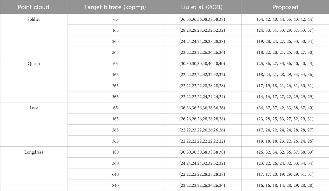
Table 1. Selection of QP values for various target bitrates. The solutions are presented in the order (QP_g,1, QP_g,2, QP_g,3, QP_g,4, QP_c,1, QP_c,2, QP_c,3, QP_c,4).

Table 2

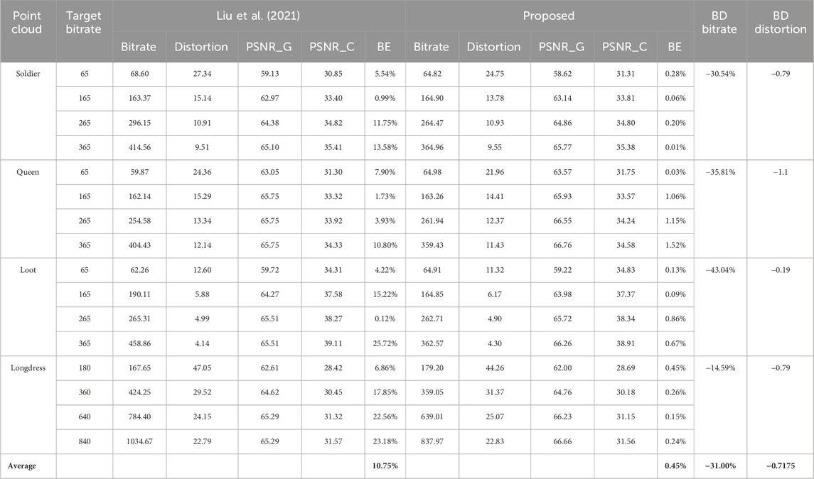
Table 2. Distortion and bitrate error for various target bitrates. The bitrates are expressed in kbpmp. The PSNRs are expressed in dB.

Figure 3

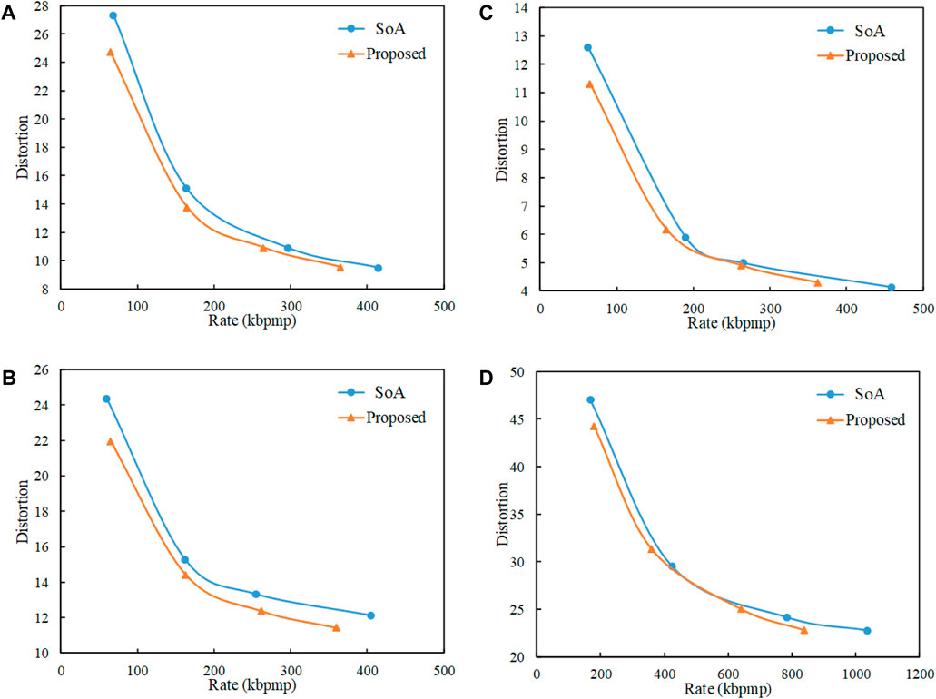
Figure 3. Comparison of the rate-distortion curves of the proposed method and the state-of-the-art method (SoA) Liu et al. (2021).(A) Soldier, (B) Queen, (C) Loot, (D) Longdress.

Figure 4 shows how the distortion decreased as a function of the number of iterations in the proposed algorithm for Loot at the target bitrate 165 kbpmp. While the distortion was still decreasing after 70 iterations, the rate of decrease was starting to stagnate.

Figure 4

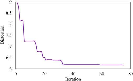
Figure 4. Distortion vs iteration number in Algorithm 1. The results are for Loot and target bitrate 165 kbpmp.

Table 3 compares the time complexity of the method in Liu et al. (2021), the proposed method, and exhaustive (full) search. For the method in Liu et al. (2021), the optimization process is based on the barrier method whose time complexity is negligible. However, there is a pre-processing step to compute the parameters of the analytical models for the distortion and rate functions. This step requires the encoding of the input point cloud three times. For the proposed method, the input point cloud is encoded at least NP times during the initialization to compute the rate and distortion of each vector in the population and NP times at each subsequent iteration to compute the rate and distortion of the offspring.

Table 3

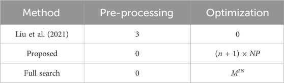
Table 3. Number of V-PCC encodings for M QP values and N frames. In the proposed algorithm, the number of generations is n and the population size is NP.

5.2 Two groups of frames

In this section, we provide results when the point cloud was encoded as two groups of frames, where each group consisted of four frames. The aim of the experiment is to show that the proposed quantization parameter optimization method can also be applied successfully when the dynamic point cloud consists of a larger number of frames. Note that optimizing the QP selection for each group of frames separately would be suboptimal, as it is unclear how to distribute the total bitrate between the first and second groups of frames. For each group of frames, we used the HEVC low-delay configuration with GOP structure IPPP. To accelerate the encoding procedure for the geometry and color videos, we limited the motion search range to 4, “MaxPartitionDepth” to 1, and the transform size to 16 in the configuration file of the HEVC encoder. In the proposed algorithm, N = 8 in (12), the size of the population was 80, the number of iterations was 150, and the range of the scaling factor was the interval [0.1, 0.9]. In the initialization step, a vector was included only if it satisfied the rate constraint, where the rate was computed according to the analytical model of the method in Yuan et al. (2021a). In the method in Liu et al. (2021), we took all eight frames of the two groups of frames as a whole to calculate the model parameters. The rate and distortion models for the eight frames were then used to compute the solution of the constrained optimization problem with the interior point method in Liu et al. (2021) for the given target bitrates. The resulting QPs for the proposed method and the method in Liu et al. (2021) are given in Table 4 for the four point clouds Soldier, Queen, Loot, and Longdress.

Table 4

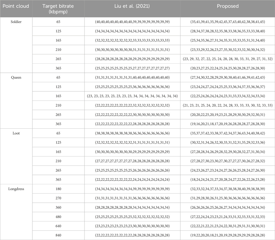
Table 4. Selection of QP values for various target bitrates when two groups of frames are encoded. The QP values for the first group are followed by those for the second group. For each group, the QP values are ordered as (QP_g,1, QP_g,2, QP_g,3, QP_g,4, QP_c,1, QP_c,2, QP_c,3, QP_c,4).

The results in Table 5 and Figure 5 demonstrate that the proposed method outperformed the state-of-the-art method Liu et al. (2021) in terms of rate-distortion performance and bitrate accuracy. For example, the BD rate was up to −10.15%, and the average BE was only 0.29%, while it reached 4.45% for the method in Liu et al. (2021). Because the HEVC video encoder configuration was simplified to reduce the encoding time, the gains shown in Table 5 are smaller than those shown in Table 2. We expect the rate-distortion gains for two groups of frames to be at least as high as for one group of frames if the same encoder configuration as in Section 5.1 is used.

Table 5

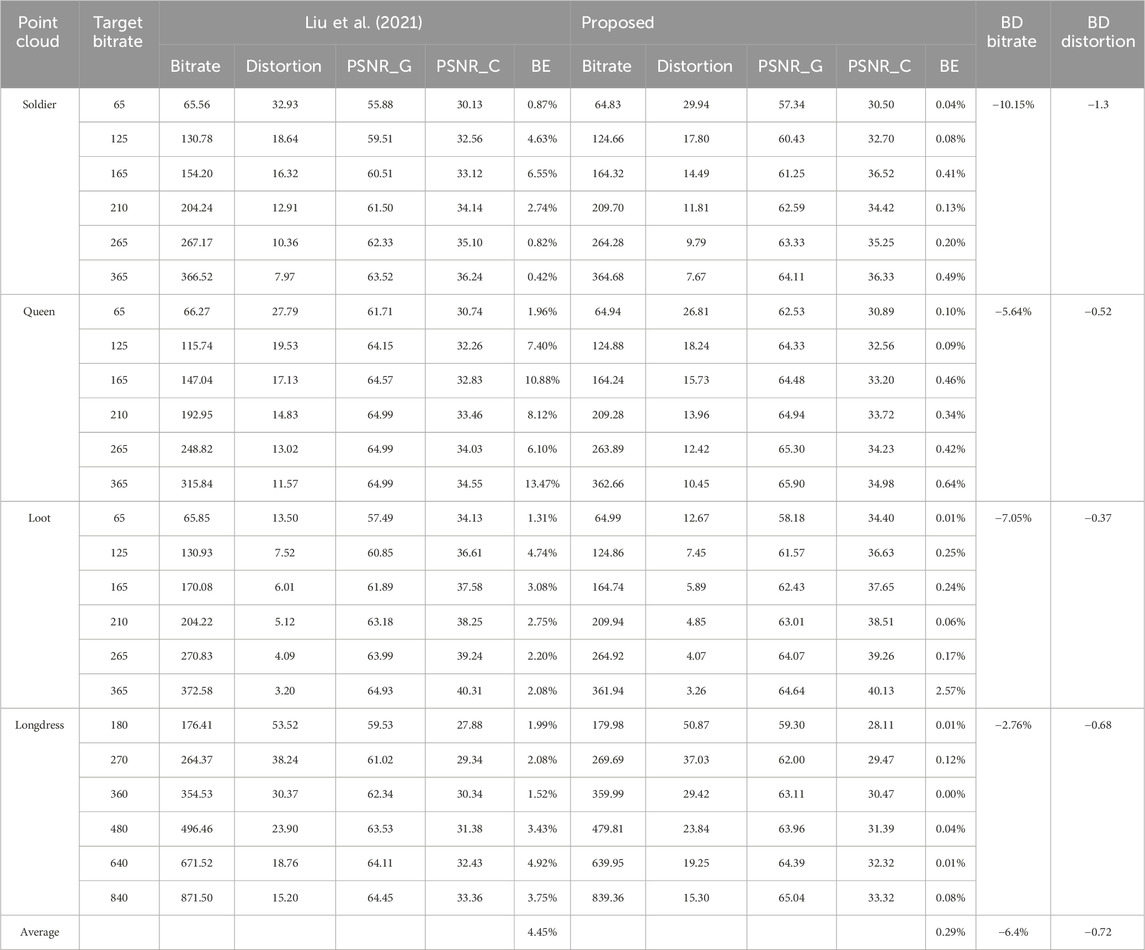
Table 5. Rate-distortion performance and bitrate accuracy (two GOPs). The bitrates are expressed in kbpmp. The PSNRs are expressed in dB.

Figure 5

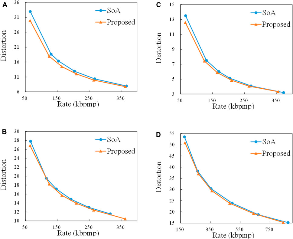
Figure 5. Comparison of the rate-distortion curves of the proposed method and the state-of-the-art method (SoA) for two GOPs. (A) Soldier, (B) Queen, (C) Loot, (D) Longdress.

5.3 Visual quality results

In this section, we compare the visual quality of the reconstructed point clouds for the proposed algorithm and the method in Liu et al. (2021). To render images of the point cloud, we used the MPEG PCC renderer software Guede et al. (2017). This tool converts the point clouds to videos based on a specified view angle. Both the width and height of the rendered videos were 480.

Figure 6 shows the results when a single group of frames was encoded as in Section 5.1. The point cloud images obtained from the proposed method had better quality than those obtained with the method in Liu et al. (2021), especially for edges and complex textures. Note that for Longdress, Queen, and Soldier the visual quality was better despite a lower encoding bitrate. This was possible because the proposed algorithm can determine the QPs for different frames flexibly based on the content of the texture.

Figure 6

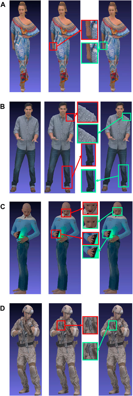
Figure 6. Visual quality comparison for one group of frames. (A) Longdress (1054th frame, i.e., fourth frame of the group. Left: original, rate = 179,943.42 kbpmp. Middle: method in Liu et al. (2021), rate = 424.25 kbpmp. Right: proposed, rate = 359.05 kbpmp). (B) Loot (1004th frame, i.e., fourth frame of the group. Left: original, rate = 173,765.31 kbpmp. Middle: method in Liu et al. (2021), rate = 62.26 kbpmp. Right: proposed, rate = 64.91 kbpmp). (C) Queen (1004th frame, i.e., fourth frame of the group. Left: original, rate = 172,007.50 kbpmp. Middle: method in Liu et al. (2021), rate = 404.43 kbpmp. Right: proposed, rate = 359.43 kbpmp). (D) Soldier (1819th frame, i.e., fourth frame of the group. Left: original, rate = 176,810.67 kbpmp. Middle: method in Liu et al. (2021), rate = 68.60 kbpmp. Right: proposed, rate = 64.82 kbpmp).

Figure 7 shows the results when two groups of frames were encoded as in Section 5.2. Here also, the visual quality of the point clouds encoded with QPs selected with the proposed algorithm was better.

Figure 7

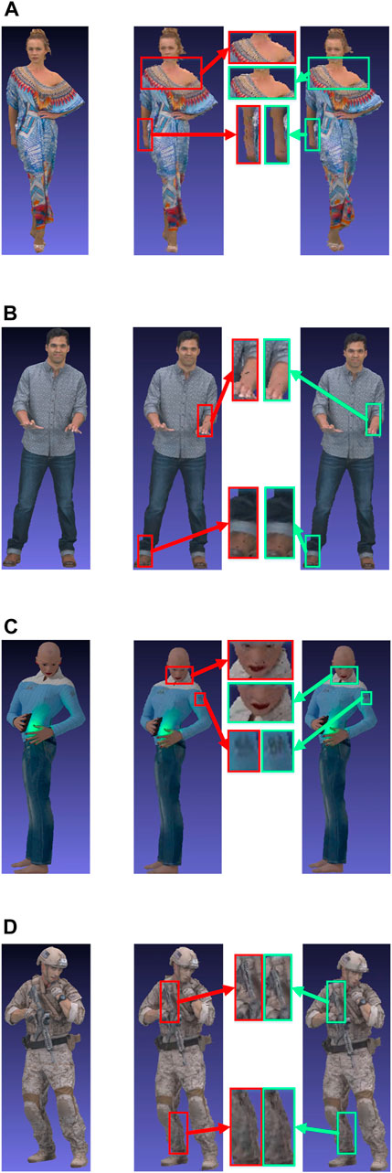
Figure 7. Visual quality comparison for two groups of frames. (A) Longdress (1058th frame, i.e., eighth frame of the two groups. Left: original, rate = 179,994.95 kbpmp. Middle: method in Liu et al. (2021), rate = 176.41 kbpmp. Right: proposed, rate = 179.98 kbpmp). (B) Loot (1008th frame, i.e., eighth frame of the two groups. Left: original, rate = 173,822.11 kbpmp. Middle: method in Liu et al. (2021), rate = 170.08 kbpmp. Right: proposed, rate = 164.74 kbpmp). (C) Queen (1008th frame, i.e., eighth frame of the two groups. Left: original, rate = 172,008.44 kbpmp. Middle: method in Liu et al. (2021), rate = 115.74 kbpmp. Right: proposed, rate = 124.88 kbpmp). (D) Soldier (1816th frame, i.e., first frame of the two groups. Left: original, rate = 176,805.24 kbpmp. Middle: method in Liu et al. (2021), rate = 65.56 kbpmp. Right: proposed, rate = 64.83 kbpmp).

5.4 Group-level optimization

In the previous sections, all CTUs within a frame were encoded using the same QP value. In this section, we extend our optimization framework by dividing the frame into groups of CTUs, allowing different groups to use distinct QP values. Figure 8 illustrates this approach. Since our original framework is a particular case where the number of groups in a frame is equal to one, we anticipate a reduction in distortion. However, the introduction of multiple QP values results in an increased bitrate. Furthermore, the complexity of the DE algorithm also rises, as the dimension of the vector x in (12) is multiplied by the number of groups. For high-dimensional problems, it is necessary to increase both the population size and the number of generations. However, a larger population size makes verifying that the vectors in the initial population meet the rate constraint more challenging. To address this issue, we apply the DE algorithm to the unconstrained problem min_xD(x) + λR(x), where λ is a Lagrange multiplier.

Figure 8

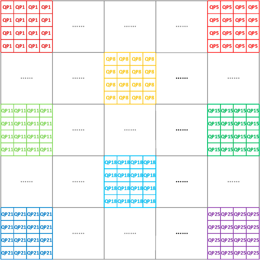
Figure 8. Frame partition into groups. A 1280 × 1280 frame is partitioned into 25 groups, each of which contains 16 CTUs of size 64 ×64.

To test the hypothesis that group-level optimization can lead to better solutions, we compared the solutions obtained with frame-level optimization (as in Section 5.1) to those obtained with group-level optimization. We used the HEVC low-delay configuration with GOP structure IPPP. To accelerate the encoding procedure for the geometry and color videos, we limited the motion search range to 4, “MaxPartitionDepth” to 1, and the transform size to 16 in the configuration file of the HEVC encoder. For frame-level optimization, the population size NP was 50, the number of generations n was 75, and the scaling factor μ was selected in the interval I = [0.1, 0.9]. The dimension of the vector in the DE algorithm was 8. For group-level optimization, each frame was split horizontally into two groups (Figure 9). Thus, the dimension of the vector was 16. In addition, we set the population size (NP) to 80 and the number of generations (n) to 150. The scaling factor was selected in the interval I = [0.1, 0.9].

Figure 9

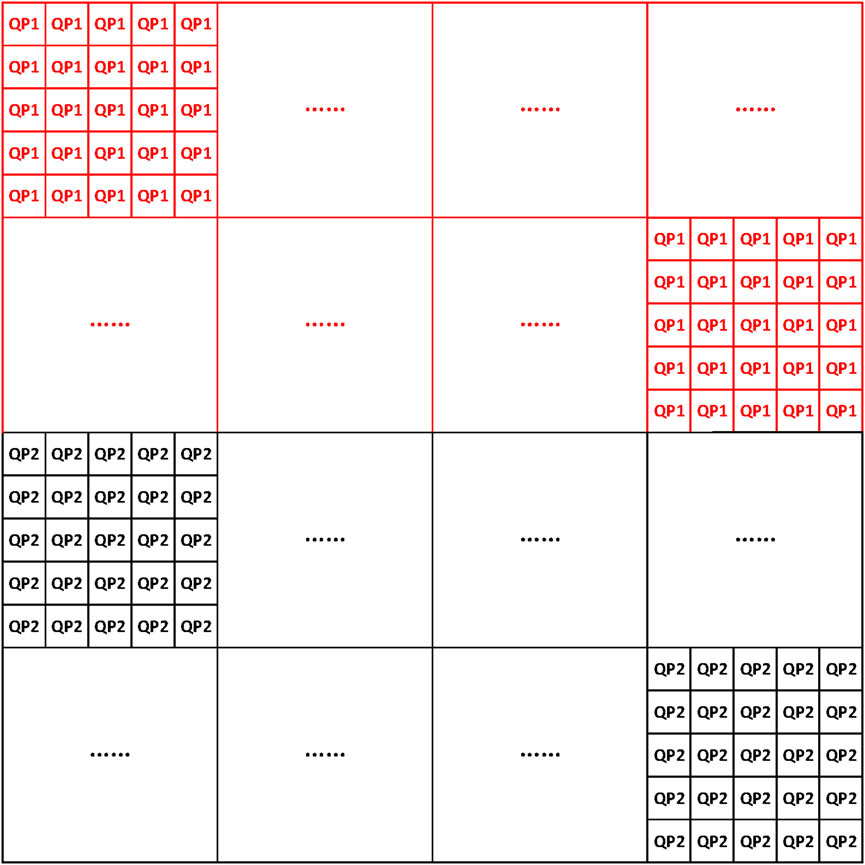
Figure 9. Frame partition into two groups. A 1280 × 1280 frame is partitioned into two groups, each of which contains 200 CTUs of size 64 × 64.

Table 6 presents the results. For the four point clouds, group-level optimization resulted in bitrate savings. Although the reduction in bitrate was small, the experiment highlights the potential of our approach.

Table 6

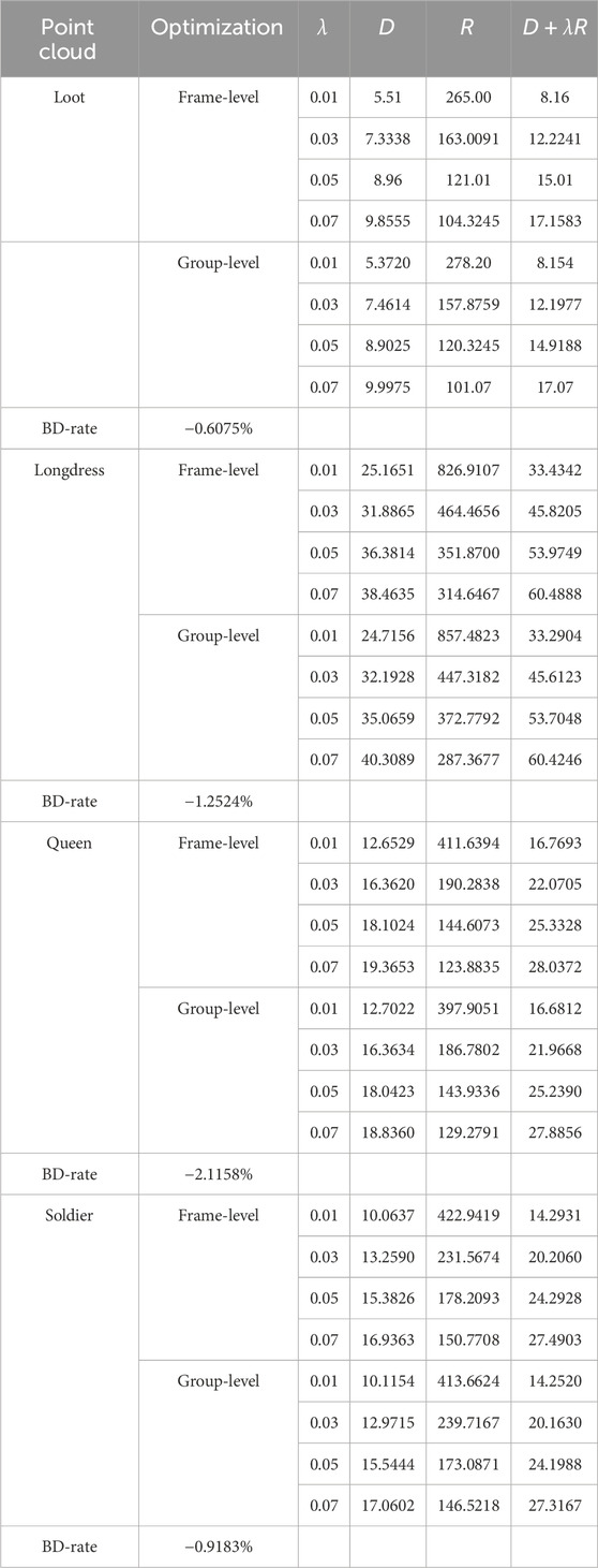
Table 6. Rate-distortion results. Frame-level optimization is used as the anchor in the BD-rate calculation. The rate is calculated in kbpmp.

Table 7 shows the QP values selected by the DE algorithm for group-level optimization. In almost all cases, the QP value selected for the first group was different from the one selected for the second group.

Table 7

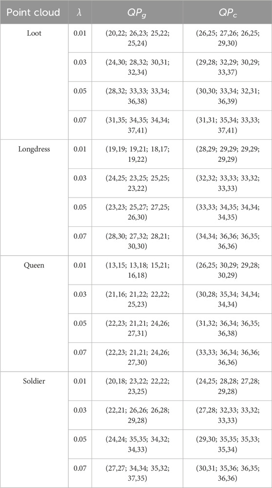
Table 7. Selected QP values. Four geometry frames and four color frames are encoded. The QP for the upper group of the first frame is listed first, followed by the QP for the bottom group of the first frame, and so on.

Table 8 compares the CPU time of the frame-level optimization and group-level optimization for the first generation of the DE algorithm when λ = 0.01. The computations were conducted on an Intel^® Xeon^® W-2255 CPU, operating at a frequency of 3.70 GHz and equipped with 128 GB of RAM. The CPU time for group-level optimization is about 1.6 times that of frame-level optimization, reflecting the ratio of their population sizes, 80:50.

Table 8

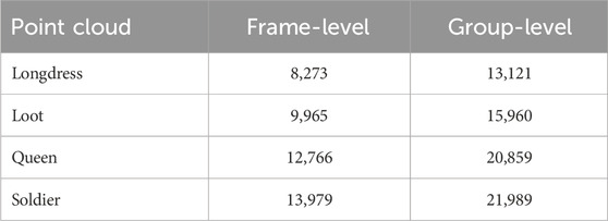
Table 8. CPU time (in s) for one iteration of frame-level optimization and group-level optimization when λ = 0.01.

6 Conclusion

We proposed a method that optimizes the selection of the QP values of the geometry video and color video for V-PCC. Extensive experimental results showed that our method can significantly improve the rate-distortion performance and the bitrate accuracy of the standard approach in which the QP values of all frames in a group of frames are assumed to be equal. In our method, the objective function and the constraint are the actual distortion and rate functions. Consequently, our method is more accurate than all previous works Li et al. (2020), Yuan et al. (2021a), Liu et al. (2021), which select the QP values by optimizing analytical models of these functions.

To tackle the optimization problem, we used a variant of the DE algorithm. Compared to the standard DE algorithm, we implemented three changes. First, we adapted the DE algorithm to the constrained combinatorial nature of the problem. Second, we decreased the crossover rate after two-thirds of the iterations to prevent stagnation of the algorithm. Third, we randomly selected the scaling factor to ensure population diversity.

Each iteration in our DE algorithm requires the encoding of the point cloud NP times. Since the V-PCC encoder has a high time complexity, we restricted the number of generations to 75 for one group of frames and 150 for two groups of frames and one group of frames with two groups. We anticipate that increasing the number of generations will lead to better results as the recommended number is higher for the population size and dimension of the problem at hand Suganthan et al. (2005). Note that because of its high complexity, our method is not suitable for real-time applications.

Future work could focus on optimizing the partitioning of a frame into groups of CTUs for group-level optimization. This optimization should account for both the geometry of the partitions and the number of partitions. Our optimization framework may lead to significant fluctuations in the QP values within a group of frames, which could negatively affect the subjective visual quality. However, this issue can be mitigated by introducing appropriate constraints on the problem variables. Finally, future research could explore more sophisticated variants of DE Das and Suganthan (2011) and other global optimization algorithms, such as genetic algorithms and particle swarm optimization.

Data availability statement

The datasets presented in this study can be found in online repositories. The names of the repository/repositories and accession number(s) can be found in the article/supplementary material.

Author contributions

HY: Conceptualization, Methodology, Writing–original draft, Investigation, Software. RH: Conceptualization, Methodology, Writing–original draft. FN: Conceptualization, Methodology, Writing–original draft. SY: Conceptualization, Methodology, Writing–review and editing. XL: Writing–review and editing, Investigation, Methodology, Software. LZ: Writing–review and editing. YZ: Conceptualization, Methodology, Writing–review and editing.

Funding

The author(s) declare that financial support was received for the research, authorship, and/or publication of this article. This work has received funding from the European Union’s Horizon 2020 research and innovation programme under the Marie Skłodowska-Curie grant agreement No. 836192, from the National Natural Science Foundation of China under grants 62222110, 62172259, and 62172400, and from the Chinese Academy of Sciences President’s International Fellowship Initiative (PIFI) under grant 2022VTA0005.

Conflict of interest

Authors HY, RH, FN, and SY hold a patent (GB2606000) related to this research.

The remaining authors declare that the research was conducted in the absence of any commercial or financial relationships that could be construed as a potential conflict of interest.

Authors HY, RH, FN, and XL declared that they were an editorial board member of Frontiers, at the time of submission. This had no impact on the peer review process and the final decision.

The reviewer ZJ declared a shared affiliation with the author YZ to the handling editor at the time of review.

Publisher’s note

All claims expressed in this article are solely those of the authors and do not necessarily represent those of their affiliated organizations, or those of the publisher, the editors and the reviewers. Any product that may be evaluated in this article, or claim that may be made by its manufacturer, is not guaranteed or endorsed by the publisher.

References

Al-Dabbagh, R. D., Neri, F., Idris, N., and Baba, M. S. (2018). Algorithmic design issues in adaptive differential evolution schemes: review and taxonomy. Swarm Evol. Comput. 43, 284–311. doi:10.1016/j.swevo.2018.03.008

CrossRef Full Text | Google Scholar

Berger, M., Tagliasacchi, A., Seversky, L., Alliez, P., Guennebaud, G., Levine, J., et al. (2017). A survey of surface reconstruction from point clouds. Comput. Graph. Forum 36, 301–329. doi:10.1111/cgf.12802

CrossRef Full Text | Google Scholar

Bjøntegaard, G. (2001). Calculation of average psnr differences between rd curves. Austin, TX, USA, April: VCEG-M33.

Google Scholar

Budagavi, M., Fuldseth, A., and Bjøntegaard, G. (2014) HEVC transform and quantization. Cham: Springer International Publishing, 141–169.

CrossRef Full Text | Google Scholar

Byrd, R. H., Hribar, M. E., and Nocedal, J. (2006). An interior point algorithm for large-scale nonlinear programming. SIAM J. Optim. 9, 877–900. doi:10.1137/s1052623497325107

CrossRef Full Text | Google Scholar

Das, S., Konar, A., and Chakraborty, U. K. (2005). “Two improved differential evolution schemes for faster global search,” in Proc. 7th Annual Conf. on Genetic and Evolutionary Computation (GECCO’05), Washington, DC, USA, June, 2005.

CrossRef Full Text | Google Scholar

Das, S., and Suganthan, P. N. (2011). Differential evolution: a survey of the state-of-the-art. IEEE Trans Evol. Comput. 15, 4–31. doi:10.1109/tevc.2010.2059031

CrossRef Full Text | Google Scholar

Fiengo, A., Chierchia, G., Cagnazzo, M., and Pesquet-Popescu, B. (2017). Rate allocation in predictive video coding using a convex optimization framework. IEEE Trans. Image Process 26, 479–489. doi:10.1109/tip.2016.2621666

PubMed Abstract | CrossRef Full Text | Google Scholar

Graziosi, D., Nakagami, O., Kuma, S., Zaghetto, A., Suzuki, T., and Tabatabai, A. (2020). An overview of ongoing point cloud compression standardization activities: video-based (v-pcc) and geometry-based (g-pcc). APSIPA Trans. Signal Inf. Process. 9. doi:10.1017/atsip.2020.12

CrossRef Full Text | Google Scholar

Guede, C., Ricard, J., Lasserre, S., and Schaeffer, R. (2017). “User manual for the pcc rendering software,” in ISO/IEC JTC1/SC29/WG11 MPEG2017/N16902 (Hobart, Australia).

Google Scholar

HoangVan, X., Dao Thi Hue, L., and Nguyen Canh, T. (2021). A trellis based temporal rate allocation and virtual reference frames for high efficiency video coding. Electronics 10, 1384. doi:10.3390/electronics10121384

CrossRef Full Text | Google Scholar

Huang, K., and Hang, H. (2009). Consistent picture quality control strategy for dependent video coding. IEEE Trans. Image Process 18, 1004–1014. doi:10.1109/tip.2009.2014259

PubMed Abstract | CrossRef Full Text | Google Scholar

ISO/IEC (2020a). “V-PCC codec description,” in ISO/IEC jtc 1/SC 29/WG 7 N00012 (Washington, DC, USA: ISO).

Google Scholar

ISO/IEC (2020b). “V-PCC test model v12,” in ISO/IEC jtc 1/SC 29/WG7 N00006 (Washington, DC, USA: ISO).

Google Scholar

Lampinen, J., and Zelinka, I. (2000). “On the stagnation of the differential evolution algorithm,” in Proc. MENDEL’00 6th International Mendel Conference on Soft Computing, Czech, Republic, July, 2000, 76–83.

Google Scholar

Li, L., Li, Z., Liu, S., and Li, H. (2020). Rate control for video-based point cloud compression. IEEE Trans. Image Process. 29, 6237–6250. doi:10.1109/TIP.2020.2989576

PubMed Abstract | CrossRef Full Text | Google Scholar

Li, X., Amon, P., Hutter, A., and Kaup, A. (2010). “Adaptive quantization parameter cascading for hierarchical video coding,” in Proc. IEEE Int. Symp. Circuits Syst. (ISCAS), Paris, France, May, 2020, 4197–4200.

CrossRef Full Text | Google Scholar

Liu, Q., Yuan, H., Hamzaoui, R., and Su, H. (2020). “Coarse to fine rate control for region-based 3d point cloud compression,” in Proc. IEEE Int. Conf. on Multimedia & Expo Workshops (ICMEW), Taipei City, Taiwan, July, 2020.

CrossRef Full Text | Google Scholar

Liu, Q., Yuan, H., Hou, J., Hamzaoui, R., and Su, H. (2021). Model-based joint bit allocation between geometry and color for video-based 3d point cloud compression. IEEE Trans. Multimedia 23, 3278–3291. doi:10.1109/tmm.2020.3023294

CrossRef Full Text | Google Scholar

Marzuki, I., and Sim, D. (2020). Perceptual adaptive quantization parameter selection using deep convolutional features for HEVC encoder. IEEE Access 8, 37052–37065. doi:10.1109/access.2020.2976142

CrossRef Full Text | Google Scholar

McCann, K., Rosewarne, C., Bross, B., Naccari, M., Sharman, K., and Sullivan, G. J. (2014). High efficiency video coding (hevc) test model 16 (hm 16) encoder description. JCTVC-R 1002.

Google Scholar

Mekuria, R., Li, Z., Tulvan, C., and Chou, P. (2016). Evaluation criteria for pcc (point cloud compression). n16332. geneva: iso/iec jtc1/sc29/wg11.

Google Scholar

Neri, F., and Tirronen, V. (2010). Recent advances in differential evolution: a survey and experimental analysis. Artif. Intell. Rev. 33, 61–106. doi:10.1007/s10462-009-9137-2

CrossRef Full Text | Google Scholar

Price, K., Storn, R. M., and Lampinen, J. A. (2005). Differential evolution: a practical approach to global optimization. Heidelberg: Springer.

Google Scholar

Ramchandran, K., Ortega, A., and Vetterli, M. (1994). Bit allocation for dependent quantization with applications to multiresolution and MPEG video coders. IEEE Trans. Image Process 3, 533–545. doi:10.1109/83.334987

PubMed Abstract | CrossRef Full Text | Google Scholar

Suganthan, P. N., Hansen, N., Liang, J. J., Deb, K., Chen, Y. P., Auger, A., et al. (2005). “Problem definitions and evaluation criteria for the CEC 2005 special session on real-parameter optimization,”. Tech. rep. Technical Report. Singapore: Nanyang Technological University.

Google Scholar

Sullivan, G., Ohm, J.-R., Han, W., and Wiegand, T. (2012). Overview of the high efficiency video coding (hevc) standard. IEEE Trans. Circuits Syst. Video Technol. 22, 1649–1668. doi:10.1109/tcsvt.2012.2221191

CrossRef Full Text | Google Scholar

Wang, T., Li, F., and Cosman, P. C. (2022). Learning-based rate control for video-based point cloud compression. IEEE Trans. Image Process. 31, 2175–2189. doi:10.1109/TIP.2022.3152065

PubMed Abstract | CrossRef Full Text | Google Scholar

Wu, C.-H., Hsu, C.-F., Hung, T.-K., Griwodz, C., Ooi, W. T., and Hsu, C.-H. (2022). Quantitative comparison of point cloud compression algorithms with pcc arena. IEEE Trans. Multimed. 25, 3073–3088. doi:10.1109/TMM.2022.3154927

CrossRef Full Text | Google Scholar

Xue, Y., Tong, Y., and Neri, F. (2022). An ensemble of differential evolution and adam for training feed-forward neural networks. Inf. Sci. 608, 453–471. doi:10.1016/j.ins.2022.06.036

CrossRef Full Text | Google Scholar

Yuan, H., Hamzaoui, R., Neri, F., and Yang, S. (2021a). “Model-based rate-distortion optimized video-based point cloud compression with differential evolution,” in Proceedings of the 11th International Conference on Image and Graphics (ICIG 2021), Haikou, China, September, 2021, 735–747.

CrossRef Full Text | Google Scholar

Yuan, H., Hamzaoui, R., Neri, F., and Yang, S. (2021b). Source code for rate-distortion optimization of video-based point cloud compression with differential evolution (1.0). Zenodo. doi:10.5281/zenodo.5552760

CrossRef Full Text | Google Scholar

Yuan, H., Hamzaoui, R., Neri, F., Yang, S., and Wang, T. (2021c) Data files for IEEE MMSP 2021 paper (1.0). Zenodo. doi:10.5281/zenodo.5211174

CrossRef Full Text | Google Scholar

Yuan, H., Hamzaoui, R., Neri, F., Yang, S., and Wang, T. (2021d). “Global rate-distortion optimization of video-based point cloud compression with differential evolution,” in Proc. 23rd International Workshop on Multimedia Signal Processing, Tampere, Finland, October, 2021.

CrossRef Full Text | Google Scholar

Zhao, T., Wang, Z., and Chen, C. W. (2016). Adaptive quantization parameter cascading in hevc hierarchical coding. IEEE Trans. Image Process. 25, 2997–3009. doi:10.1109/tip.2016.2556941

PubMed Abstract | CrossRef Full Text | Google Scholar