Voice synthesis using power-balanced simulation of a quasi-1D model of the vocal apparatus

The vocal apparatus is a biophysical dynamic system capable of self-oscillation, which involves fluid–structure interactions and human control. This study on the sound synthesis of voiced sounds presents a physical quasi-1D model of the vocal apparatus in the port-Hamiltonian framework and its validation through numerical experiments. The modelling ensures balanced power exchanges between fluid, tissues, and human control. Fluid is represented in the larynx and in the vocal tract using a unified 1D PDE handling transverse geometry variations. A regularisation procedure is introduced to mitigate the numerically stiff behaviour of the model observed at channel closure. Vocal folds and vocal tract walls are represented by lumped element models as well as the radiation load at the lips, which consists of a first-order high-pass filter. Spatial discretisation of the fluid model and temporal discretisation of the full system are made using structure-preserving methods to ensure energy consistency (passivity). The second part of this paper focuses on numerical experiments to progressively characterise the model and assess its validity. These experiments begin with frequency response analysis of a static vocal tract under quasi-linear conditions followed by simulations of vowel transitions (diphthongs) under forced excitation. Next, self-oscillation studies are conducted on an isolated larynx where contact parameters are adjusted. Lastly, full simulations of the self-oscillating vocal apparatus with co-articulation, representing a voice synthesizer capable of articulating vowels, are presented. The dynamics are also analysed in terms of energy transfer and passivity. Finally, these results are discussed to establish a basis for future model refinements and to identify directions for enhancing the accuracy and realism of vocal synthesis.

1 Introduction

Understanding the mechanisms of voice production has been the focus of numerous studies on the physical modelling of the vocal apparatus. Highly detailed models that capture the range of physically relevant phenomena typically involve high-dimensional representations, which can be computationally intensive. Consequently, these studies often focus on specific components or aspects of the vocal apparatus (e.g., Alipour et al., 2000; Gunter, 2003; Xue et al., 2010; Guasch et al., 2013; Zhang, 2015; Valášek, 2021). In contrast, low-order models aim to replicate the qualitative behaviour of the vocal apparatus along with certain quantitative features (such as the relationship between subglottal pressure and fundamental frequency, as demonstrated in Ruty et al. (2007)) while maintaining relatively low computational costs. This computationally efficient approach has been a key focus since the early days of sound synthesis, with foundational models like the Kelly–Lochbaum model (Kelly, 1962) or digital implementations of lumped-parameter physical models (e.g., Maeda, 1982) for the vocal tract. These models are well-suited for vocal synthesizer applications or parameter studies. For the laryngeal part, low-order models (e.g., Ishizaka and Flanagan, 1972; Story and Titze, 1994; see also the review in Erath et al., 2013) typically represent the vocal folds as assemblies of lumped mass-spring-damper elements and assume a quasi-steady behaviour of fluid flow in the glottis. However, this approach introduces a one-way coupling between the flow and the vocal folds, limiting the model’s ability to accurately represent power exchanges between the fluid and tissue, and it may introduce instabilities in numerical simulations.

Recent efforts have focused on developing power-balanced, reduced-order models of voice production within the port-Hamiltonian (pH) framework first introduced in Maschke and van der Schaft (1992). Notably, Encina et al. (2015) reformulated the body-cover vocal fold model from Story and Titze (1994), and early self-oscillating power-balanced models were introduced in Hélie and Silva (2017) and Mora et al. (2018) using lumped representations of glottal flow. Subsequent research by Mora et al. (2021b) and Wetzel (2021) proposed discrete, scalable models of compressible fluid within tubes with moving boundaries, tailored for vocal tract applications. However, this set of studies primarily focused on isolated larynx models (possibly coupled with an oversimplified acoustic load) or on isolated vocal tracts under basic configurations.

This paper presents a complete simplified power-balanced model of the vocal apparatus within the pH framework, designed for the synthesis of voiced sounds. A one-dimensional distributed fluid model is developed and described as a port-Hamiltonian system of partial differential equations, accounting for compressibility, time-varying geometry, and convective acceleration. A new regularisation procedure for handling glottal closure is introduced. This model is then spatially discretised in a structure-preserving manner, from which the discrete fluid model from Mora et al. (2021b) is recovered. The vocal fold model is based on the lumped-element body-cover model from Story and Titze (1994), while the vocal tract walls are represented by a series of simpler mass-spring damper systems. At the lips, the radiation condition is modelled as an impedance load, represented by a first-order high-pass filter, tuned according to acoustic considerations and designed to be passive and compatible with time-varying configurations. Each component is formulated within the pH framework and interconnected via ports using a two-way coupling, ensuring a global power balance. Simulations are performed using an energy-preserving time integration method across various configurations, including the vocal tract alone, the larynx alone, and the complete assembly. Notably, the ability of the complete model to reproduce the co-articulation of diphthongs in self-oscillating configurations is demonstrated—an achievement that, to the best of our knowledge, is unprecedented in the context of energy-based modelling of voice production. Energy-based modelling explicitly reveals the power exchanges and dissipated power signals, which are discussed in detail.

After positioning our contributions within the existing literature on voice production modelling in Section 1, the remainder of this paper is organised as follows. Section 2 introduces the fluid and tissue models used in the experiments. Section 3 presents a series of numerical experiments based on these models, progressively increasing in complexity and realism, to assess their validity and capabilities. Finally, Section 4 discusses the results and outlines potential directions for future work.

2 Model

Energy-based models for fluid dynamics and vocal folds are proposed within the port-Hamiltonian framework. These models are subsequently interconnected, resulting in power-preserving fluid–structure interactions. Symmetry around the laryngeal midplane is assumed, allowing reduction of the problem to the case of a single vocal fold and simplifying the presentation.

2.1 Fluid flow model

The modelling of the fluid flow is proposed within the framework of port-Hamiltonian systems. It relies on the strict separation of the intrinsic behaviour of the fluid (described by means of the Hamiltonian, summing up kinetic energy and internal energy, or more specifically by the fluid behaviour law relating the pressure to the mass density) from the evolution laws (provided as mass and momentum conservation laws). As an original contribution of this paper, the latter are formulated as 1D partial differential equations under a detailed set of assumptions. Spatial discretisation is applied to obtain a discrete model, similar to that used in Mora et al. (2021b), with the change of state variables proposed in Risse et al. (2024). Here, the model with this revised set of state variables is presented. The model is constructed as a conservative system (the energy conservation naturally derives from the port-Hamiltonian systems), and lumped dissipation laws are added after spatial discretisation.

2.1.1 Formulation as a continuous 1D PDE system

The time-varying fluid domain is described in 3D cartesian space as follows:

$\mathrm{\Omega }\left(t\right)=\left\{\xi =\left(x,y,z\right)|x\in \left(0,l_0\right),y\in \left(0,h\left(x,t\right)\right),z\in \left(0,L_0\right)\right\}.(1)$

Figure 1 presents the domain as well as its boundaries. Boundaries ${\partial }_{\mathrm{\Omega }}^L$ and ${\partial }_{\mathrm{\Omega }}^R$ represent the inlet and outlet of the tube through which fluid can flow. In contrast, ${\partial }_{\mathrm{\Omega }}^A$ denotes a rigid, sealed, and impermeable boundary, while ${\partial }_{\mathrm{\Omega }}^B$ corresponds to a mobile impervious fluid–structure interface.

Figure 1

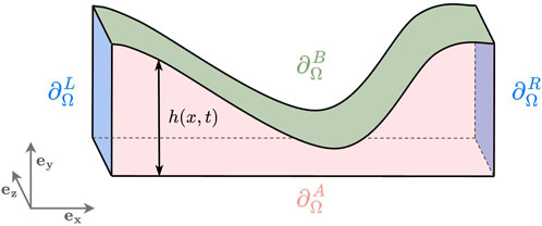
Figure 1. Fluid domain $\mathrm{\Omega }(t)$ and associated boundaries.

The following assumptions are made for the fluid in $\mathrm{\Omega }(t)$:

Hypothesis 1. The fluid is composed of an ideal gas (H1a) undergoing homentropic flow (i.e., constant entropy in space and time) (H1b).

Hypothesis 2. The fluid is inviscid.

Hypothesis 3. The flow is irrotational.

Let $\mathbf{v}$ denote the fluid velocity, $\rho$ the volumetric mass density, $P$ the pressure, and $u$ the specific internal energy (i.e., the internal energy per unit mass). The specific enthalpy is defined as $\mathfrak{h}=u+\frac{P}{\rho }$, while the total specific enthalpy is ${\mathfrak{h}}_{\text{tot}}=\frac{1}{2}{\mathbf{v}}^2+\mathfrak{h}$. Accounting for the fundamental thermodynamic relation $\mathrm{d}u(\rho ,s)=-P(\rho ,s)\mathrm{d}\left(1/\rho \right)+T(\rho ,s)\mathrm{d}s$ and for hypothesis (H1b) (with constant specific entropy $s=s_0$, i.e., $\mathrm{d}s\equiv 0$), the pressure $P$, temperature $T$, specific internal energy $u$, and specific enthalpy $\mathfrak{h}$ depend effectively on $\rho$ only with

$\left(a\right):\mathrm{d}u\left(\rho \right)=-P\left(\rho \right)d\left(1/\rho \right)=\frac{P\left(\rho \right)}{{\rho }^2}\mathrm{d}\rho \iff \left(b\right):\frac{1}{\rho }\mathrm{d}P\left(\rho \right)=\mathrm{d}\mathfrak{h}\left(\rho \right).(2)$

Under Hypotheses 2 and 3, Euler equations for irrotational flow in the domain $\mathrm{\Omega }$ can be written as

${\partial }_t\rho +\text{div}\left(\rho \mathbf{v}\right)=0\left(\text{mass\hspace{0.17em}equation}\right),(\mathrm{3a})$

${\partial }_t\mathbf{v}+\underset{\stackrel{\left(2b\right)}{=}\mathbf{g}\mathbf{r}\mathbf{a}\mathbf{d}\left({\mathfrak{h}}_{\mathit{tot}}\right)}{\underbrace{\mathbf{g}\mathbf{r}\mathbf{a}\mathbf{d}\left(\frac{1}{2}{\mathbf{v}}^2\right)+\frac{1}{\rho }\mathbf{g}\mathbf{r}\mathbf{a}\mathbf{d}\left(P\right)}}=0\left(\text{momentum\hspace{0.17em}equation}\right).(\mathrm{3b})$

To close the system of equations, thermodynamic considerations are used to provide expressions for functions $P(\rho )$ and $u(\rho )$. The following additional hypothesis is used, which provides a valid approximation within the amplitude range of typical voice pressure signals.

Hypothesis 4. The function $\rho \mapsto P(\rho )$ is linearised around the equilibrium at rest, with ${\rho }_0$ and $P_0=P({\rho }_0)$ and assuming $P(\rho )-P_0=c_0^2(\rho -{\rho }_0)$.

The corresponding expression for the specific internal energy (i.e. per unit mass) $u(\rho )$ is obtained by integrating Equation 2 from $u_0=u({\rho }_0)$, yielding $u(\rho )-u_0=c_0^2\ln \left(\rho /{\rho }_0\right)+\left(P_0-c_0^2{\rho }_0\right)\left(1/{\rho }_0-1/\rho \right)$. The enthalpy is then given by $\mathfrak{h}(\rho )\equiv \partial \left(\rho u(\rho )\right)/\partial \rho ={\mathfrak{h}}_0+c_0^2\ln \left(\rho /{\rho }_0\right)$. Note that the choice of constants $P_0$, $u_0$, and ${\mathfrak{h}}_0$ does not affect the dynamics of the fluid system. In the numerical experiments, pressure fluctuations $\widehat{P}=P-P_0$ and enthalpy fluctuations $\widehat{\mathfrak{h}}=\mathfrak{h}-{\mathfrak{h}}_0$ are used, ensuring that the resulting values and interpretations remain independent of these constants.¹

We now explicitly consider the fluid flow in the geometry depicted in Figure 1 and perform the 1D reduction. The boundary conditions are as follows. Boundaries ${\partial }_{\mathrm{\Omega }}^L$ and ${\partial }_{\mathrm{\Omega }}^R$ will be forced by either a prescribed enthalpy or a prescribed mass flow. At the sealed impermeable boundary ${\partial }_{\mathrm{\Omega }}^A$, the normal component of the fluid velocity is zero. At the mobile fluid–structure interface ${\partial }_{\mathrm{\Omega }}^B$, the continuity of normal velocity and stress is assumed. The 3D equations are reduced to a set of 1D equations by making the following additional assumptions and integrating over a section $S(x_0,t)=\{\alpha \in \mathrm{\Omega }(t)\mid x=x_0\}$ with area $\bar{S}(x,t)=L_{0}h(x,t)$.

Hypothesis 5. $v_z=0$ in $\mathrm{\Omega }$

Hypothesis 6. The fluid–structure interfaces ${\partial }_{\mathrm{\Omega }}^A$ and ${\partial }_{\mathrm{\Omega }}^B$ are impervious, meaning that the normal velocity components of the boundary and fluid are equal—$\mathbf{w}\cdot \mathbf{n}=\mathbf{v}\cdot \mathbf{n}$—where $\mathbf{w}$ represents the boundary velocity and $\mathbf{n}$ is the unit normal to the boundary.

Hypothesis 7. The contribution of the transverse velocity $v_y$ to the kinetic energy $1/2\rho \mathbf{v}\cdot \mathbf{v}$ is negligible.

Hypothesis 8. $v_x$ and $\rho$ are independent of the $y$ and $z$ coordinates. This assumption corresponds to a plane wave model in acoustics.

Hypothesis 9. The moving boundary ${\partial }_{\mathrm{\Omega }}^B$ has no component in the $x$ direction $\mathbf{w}=w_y{\mathbf{e}}_{\mathbf{y}}=\dot{h}{\mathbf{e}}_{\mathbf{y}}$.

Mass equation: considering a cross-section $S(x)$ of area $\bar{S}$ and introducing the linear mass density $\mu =\rho \bar{S}$ and the axial mass flow $q_x=\bar{S}\rho v_x$, the integration of Equation 3a over $S$ yields, using Hypotheses 5 and 6),²

${\partial }_t\mu +{\partial }_x{q}_x=0.(4)$

Axial momentum equation: the integration of Equation 3b and the use of Hypotheses 7 and 8 yield

${\partial }_t{v}_x+{\partial }_x{\mathfrak{h}}_{\mathit{tot}}=0.(5)$

The distributed state ${\mathit{\alpha }}_f^{1\text{D}}={[v_x,\mu ,h]}^{⊺}$ is introduced, from which the Hamiltonian (energy of the system) is written as the sum of kinetic and compression energies (valid for $\mu \ge 0$ and $h\ge 0$).

${\mathcal{H}}_f^{1\text{D}}\left({\mathit{\alpha }}_f^{1\text{D}}\right)={\int }_0^{l_0}\left[\frac{1}{2}\mu v_x^2+\mu u\left(\frac{\mu }{L_{0}h}\right)\right]dx.(6)$

Efforts are obtained as variational derivatives of the Hamiltonian with respect to the state variables (e.g., Olver, 1986, chapter 4, for a definition of variational derivative).

${\delta }_{v_x}{\mathcal{H}}_f^{1\text{D}}=\mu v_x≕q_x,{\delta }_{\mu }{\mathcal{H}}_f^{1\text{D}}=\frac{1}{2}{v}_x^2+\mathfrak{h}≕{\mathfrak{h}}_{\mathit{tot}},{\delta }_h{\mathcal{H}}_f^{1\text{D}}=-L_0{\rho }^2{u}^{\prime }\left(\rho \right)≕-L_{0}P.(7)$

The pH formulation including the dynamics of the geometry configuration given by Hypothesis 9 then reads

$\left[\begin{array}{c}\hfill {\partial }_t{v}_x\hfill \\ \hfill {\partial }_t\mu \hfill \\ \hfill {\partial }_{t}h\hfill \\ \hfill y_{\mathit{dis}}=L_{0}P\hfill \end{array}\right]=\left[\begin{array}{cccc}\hfill 0\hfill & \hfill -{\partial }_x\hfill & \hfill 0\hfill & \hfill 0\hfill \\ \hfill -{\partial }_x\hfill & \hfill 0\hfill & \hfill 0\hfill & \hfill 0\hfill \\ \hfill 0\hfill & \hfill 0\hfill & \hfill 0\hfill & \hfill 1\hfill \\ \hfill 0\hfill & \hfill 0\hfill & \hfill -1\hfill & \hfill 0\hfill \end{array}\right]\left[\begin{array}{cc}\hfill {\delta }_{v_x}{\mathcal{H}}_f^{1\text{D}}\hfill & \hfill =q_x\hfill \\ \hfill {\delta }_{\mu }{\mathcal{H}}_f^{1\text{D}}\hfill & \hfill ={\mathfrak{h}}_{\mathit{tot}}\hfill \\ \hfill {\delta }_h{\mathcal{H}}_f^{1\text{D}}\hfill & \hfill =-L_{0}P\hfill \\ \hfill u_{\mathit{dis}}\hfill & \hfill =w_y\hfill \end{array}\right],(8)$

where the velocity $u_{\mathit{dis}}=w_y$ of the boundary ${\partial }_{\mathrm{\Omega }}^B$ is used as a distributed input for the system, and the corresponding power conjugated output is given by $y_{\mathit{dis}}=$ −L₀P. In addition to this distributed fluid–structure interaction, boundary conditions have to be defined at the open boundaries ${\partial }_{\mathrm{\Omega }}^L$ and ${\partial }_{\mathrm{\Omega }}^R$. The power balance over the domain is expressed as a function of the trace of the efforts at the boundaries:

$\frac{d}{dt}{\mathcal{H}}_f^{1\text{D}}={\int }_0^{l_0}{\left({\delta }_{{\mathit{\alpha }}_f^{1\text{D}}}{\mathcal{H}}_f^{1\text{D}}\right)}^{⊺}{\dot{\mathit{\alpha }}}_f^{1\text{D}}dx=-{\left[q_x{\mathfrak{h}}_{\mathit{tot}}\right]}_0^{l_0}-L_0{\int }_0^{l_0}P{w}_{y}dx,(9)$

Splitting the exchanged power into a distributed contribution ${\int }_0^{l_0}{y}_{\mathit{dis}}{u}_{\mathit{dis}}dx$ due to the variation of geometry and contributions $q_x(0){\mathfrak{h}}_{\mathit{tot}}(0)$ and $q_x(l_0){\mathfrak{h}}_{\mathit{tot}}(l_0)$ of the incoming and outgoing fluid flows at the open ends of the tube. As we considered nonlinear effects in the momentum conservation, power flows at the open boundaries correspond to the product of total enthalpy and mass flow. Linearisation of the system would yield the usual acoustic power flow as a product of volume flow and pressure. In general, three configurations of open ends are to be considered:

(C0) Total enthalpy control on both sides, with mass flows as power-conjugated outputs.

(C1) Mass flow control on both sides, with total specific enthalpies as power conjugated outputs.

(C2) Mixed boundary conditions—(C0) on one side, (C1) on the other.

Remark 1. The reduction from 3D equations to a 1D reduced model involved the definition of a new state variable $h$ describing the geometry of the channel. In this respect, the procedure used and the resulting 1D equations are reminiscent of the shallow water equations.

2.1.2 Spatial discretisation: finite differences on staggered grids

The 1D continuous equation is semi-discretised using a power-preserving finite difference approximation on a staggered grid (Trenchant et al., 2018). For the sake of brevity, only the configuration (C1) where mass flows inputs are considered at both ends of the domain is detailed here, but other configurations can be obtained using the same procedure. The 1D mesh is first presented, and then field approximations are made on that mesh. The resulting dynamics obtained from injection of these approximations in Equation 8 and integration on mesh volumes are presented using a set of chosen discrete state variables.

2.1.2.1 Meshing of the 1D domain

• The domain is divided in a primal grid of $N$ sub-intervals (or edges) $\mathbf{e}=\{e_0,\dots ,e_{N-1}\}$ of lengths ${\mathbf{l}}_d={[l_{d0},\dots ,l_{dN-1}]}^{⊺}$, yielding $N+1$ nodes $\mathbf{x}={[x_0,\dots ,x_N]}^{⊺}$, including boundary nodes.

• The dual grid is built from the primal grid. Its $N+2$ nodes are defined as $\tilde{\mathbf{x}}={[x_0,{\tilde{x}}_0,\dots ,{\tilde{x}}_{N-1},x_N]}^{⊺}={[x_0,{(A\mathbf{x})}^{⊺},x_N]}^{⊺}$ using the averaging operator

$A=\frac{1}{2}\left[\begin{array}{ccccc}\hfill 1\hfill & \hfill 1\hfill & \hfill \hfill & \hfill \hfill & \hfill \left(0\right)\hfill \\ \hfill \hfill & \hfill \ddots \hfill & \hfill \ddots \hfill & \hfill \hfill \\ \hfill \hfill & \hfill \ddots \hfill & \hfill \ddots \hfill & \hfill \hfill \\ \hfill \left(0\right)\hfill & \hfill \hfill & \hfill \hfill & \hfill 1\hfill & \hfill 1\hfill \end{array}\right]\in {\mathbb{R}}^{N\times \left(N+1\right)}.(10)$

A total of $N+1$ edges $\tilde{\mathbf{e}}=\{{\tilde{e}}_0,\dots ,{\tilde{e}}_N\}$ of lengths ${\tilde{\mathbf{l}}}_d=A^{⊺}{\mathbf{l}}_d={[{\tilde{l}}_{d0},\dots ,{\tilde{l}}_{dN}]}^{⊺}$ are naturally obtained for the dual grid (Figure 2).

Figure 2

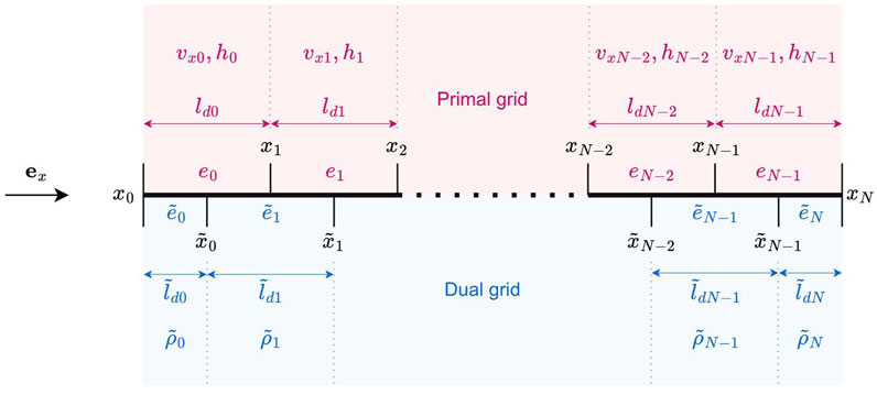
Figure 2. Staggered grid discretisation with notations for the primal grid (upper part) and dual grid (lower part).

Remark 2. We introduce the notations for Hadamard (elementwise) operations on vectors: multiplication ${(a\odot b)}_i=a_i{b}_i$, division ${(a\oslash b)}_i=a_i/b_i$, and exponentiation ${(a^{°2})}_i={(a_i)}^2$.

2.1.2.2 Approximation of the fields

• Velocity $v_x(x,t)$ and height $h(x,t)$ are assumed to be piecewise constant on edges of the primal grid and are denoted by their discrete values:

${\mathit{v}}_x\left(t\right)={\left[v_{x,0}\left(t\right),\dots ,v_{x,N-1}\left(t\right)\right]}^{⊺}\in {\mathbb{R}}^N,\text{\hspace{0.17em}and\hspace{0.17em}}\mathit{h}\left(t\right)={\left[h_0\left(t\right),\dots ,h_{N-1}\left(t\right)\right]}^{⊺}\in {\mathbb{R}}^N.(\mathrm{11a})$

The choice of discretisation for $h(x,t)$ allows the definition of volumes of fluid associated with edges of the primal grid $\mathit{V}(\mathit{h})=L_0{\mathit{l}}_d\odot \mathit{h}$ and of the dual grid $\tilde{\mathit{V}}(\mathit{h})=A^{⊺}\mathit{V}(\mathit{h})$.³

• Volumetric mass density $\rho (x,t)$ is assumed to be piecewise constant on edges of the dual grid with the set of discrete values:

$\tilde{\mathit{\rho }}\left(t\right)=\left[{\tilde{\rho }}_0\left(t\right),\dots ,{\tilde{\rho }}_N\left(t\right)\right]\in {\mathbb{R}}^{N+1}.(\mathrm{11b})$

2.1.2.3 Choice of state variables and discrete Hamiltonian

The state is chosen to be

${\mathit{\alpha }}_f={\left[{\mathit{\nu }}^{⊺},{\tilde{\mathit{m}}}^{⊺},{\mathit{h}}^{⊺}\right]}^{⊺},(12)$

with the degrees of freedom of velocity $\mathit{\nu }(t)={\mathit{l}}_d\odot {\mathit{v}}_x(t)\in {\mathbb{R}}^N$ on the primal grid and of masses of fluid $\tilde{\mathit{m}}(t)=\tilde{\mathit{V}}(\mathit{h})\odot \tilde{\mathit{\rho }}(t)\in {\mathbb{R}}^{N+1}$ in the volumes of the dual grid. This choice is motivated by the simplicity of the port-Hamiltonian formulation resulting from it and has no impact on the dynamics of the system.

The energy of the discrete fluid system is obtained by injecting field approximations in Equation 6, yielding

$H_f\left({\mathit{\alpha }}_f\right)=\frac{1}{2}{\left(\mathit{\nu }\oslash {\mathit{l}}_d\right)}^{⊺}\mathrm{d}\mathrm{i}\mathrm{a}\mathrm{g}\left(\mathit{m}(\tilde{\mathit{m}},\mathit{h})\right)\left(\mathit{\nu }\oslash {\mathit{l}}_d\right)+{\tilde{\mathit{m}}}^{⊺}u\left(\tilde{\mathit{\rho }}\right),(13)$

making use of functions of the state variables to reconstruct the volumetric mass densities in volumes of the dual grid $\tilde{\mathit{\rho }}(\tilde{\mathit{m}},\mathit{h})=\tilde{\mathit{m}}\oslash \tilde{\mathit{V}}(\mathit{h})$ and primal grid $\mathit{\rho }(\tilde{\mathit{m}},\mathit{h})=A\tilde{\mathit{\rho }}(\tilde{\mathit{m}},\mathit{h})$ and the masses of fluid in volumes of the primal grid $\mathit{m}(\tilde{\mathit{m}},\mathit{h})=\mathit{V}(\mathit{h})\odot \left(A\tilde{\mathit{\rho }}(\tilde{\mathit{m}},\mathit{h})\right)$. We also introduce the function of the state reconstructing the mean squared velocity in volumes of the dual grid $\widetilde{{\mathit{v}}^2}(\mathit{\nu },\mathit{h})=\left(A\left(\mathit{h}\odot {\mathit{\nu }}^{◦2}\oslash {\mathit{l}}_d\right)\right)\oslash \left(A(\mathit{h}\odot {\mathit{l}}_d)\right)$. Effort are naturally obtained as the gradient of the Hamiltonian:

${\partial }_{\mathit{\nu }}{H}_f=\mathit{m}(\tilde{\mathit{m}},\mathit{h})\odot \mathit{\nu }\oslash {\mathit{l}}_d^{◦2}=:\mathit{q},(\mathrm{14a})$

${\partial }_{\tilde{\mathit{m}}}{H}_f=\frac{1}{2}\mathrm{d}\mathrm{i}\mathrm{a}\mathrm{g}\left(1\oslash \tilde{\mathit{V}}(\mathit{h})\right)A^{⊺}\left(\mathit{V}(\mathit{h})\odot {\mathit{\nu }}^{◦2}\oslash {\mathit{l}}_d^{◦2}\right)+u\left(\tilde{\mathit{\rho }}\right)+\left(\tilde{\mathit{\rho }}\odot u^{\prime }\left(\tilde{\mathit{\rho }}\right)\right)=:{\tilde{\mathfrak{h}}}_{\mathit{tot}},(\mathrm{14b})$

${\partial }_{\mathit{h}}{H}_f=-L_0{\mathit{l}}_d\odot \left[A\left({\tilde{\mathit{\rho }}}^2\odot u^{\prime }\left(\tilde{\mathit{\rho }}\right)\right)-\frac{1}{2}\left(A\left(\tilde{\mathit{\rho }}\odot \widetilde{{\mathit{v}}^2}(\mathit{\nu },\mathit{h})\right)-\left(\mathit{\rho }\odot {\mathit{\nu }}^{◦2}\oslash {\mathit{l}}_d^{◦2}\right)\right)\right]=:-{\mathbf{F}}_c,(\mathrm{14c})$

and provide the mass flow rates $\mathit{q}$ averaged over the volumes of the primal grid, the enthalpy ${\tilde{\mathfrak{h}}}_{\mathit{tot}}$ averaged over the volumes of the dual grid, and the net reaction force ${\mathbf{F}}_c$ of the fluid at the fluid-structure interfaces of the primal grid.

2.1.2.4 Semi-discrete dynamical system

Injecting the field approximations in the 1D conservation equations and integrating Equation 3b on the edges of the primal grid and Equation 3a on the edges of the dual grid yields the semi-discrete dynamical system. one obtains the port-Hamiltonian formulation:

$\left[\begin{array}{c}\hfill {\partial }_t\mathit{\nu }\hfill \\ \hfill {\partial }_t\tilde{\mathit{m}}\hfill \\ \hfill {\partial }_t\mathit{h}\hfill \end{array}\right]=-\underset{J_f}{\underbrace{\left[\begin{array}{ccc}\hfill 0\hfill & \hfill D^{-}\hfill & \hfill 0\hfill \\ \hfill D^{+}\hfill & \hfill 0\hfill & \hfill 0\hfill \\ \hfill 0\hfill & \hfill 0\hfill & \hfill 0\hfill \end{array}\right]}}\left[\begin{array}{c}\hfill {\partial }_{\mathit{\nu }}{H}_f=\mathit{q}\hfill \\ \hfill {\partial }_{\tilde{\mathit{m}}}{H}_f={\tilde{\mathfrak{h}}}_{\mathit{tot}}\hfill \\ \hfill {\partial }_{\mathit{h}}{H}_f=-{\mathbf{F}}_c\hfill \end{array}\right]+G_f{\mathbf{u}}_f,(15)$

where ${\mathbf{u}}_{\mathbf{f}}={[q_{in},q_{\mathit{out}},{\mathbf{w}}_y^{⊺}]}^{⊺}$ is the input vector composed of the ingoing mass flow $q_{in}$ at $x=x_0$, outgoing mass flow $q_{\mathit{out}}$ at $x=x_N$, and fluid structure interface velocities ${\mathbf{w}}_y$. The finite difference matrix $D^{-}=-{(D^{+})}^{⊺}\in {\mathbb{R}}^{N\times (N+1)}$ and the input matrix $G_f\in {\mathbb{R}}^{(3N+1)\times (3N)}$ are written as

$D^{-}=\left[\begin{array}{ccccc}\hfill -1\hfill & \hfill 1\hfill & \hfill \hfill & \hfill \hfill & \hfill \left(0\right)\hfill \\ \hfill \hfill & \hfill \ddots \hfill & \hfill \ddots \hfill & \hfill \hfill \\ \hfill \hfill & \hfill \hfill & \hfill \ddots \hfill & \hfill \ddots \hfill \\ \hfill \left(0\right)\hfill & \hfill \hfill & \hfill \hfill & \hfill -1\hfill & \hfill 1\hfill \end{array}\right],G_f=\left[\begin{array}{ccc}\hfill 0_{N,1}\hfill & \hfill 0_{N,1}\hfill & \hfill 0_{N,N}\hfill \\ \hfill G_{ml}\hfill & \hfill G_{mr}\hfill & \hfill 0_{N+1,N}\hfill \\ \hfill 0_{N,1}\hfill & \hfill 0_{N,1}\hfill & \hfill {\mathbf{I}}_{N,N}\hfill \end{array}\right],G_{ml}=\left[\begin{array}{c}\hfill 1\hfill \\ \hfill 0\hfill \\ \hfill ⋮\hfill \\ \hfill 0\hfill \end{array}\right],G_{mr}=\left[\begin{array}{c}\hfill 0\hfill \\ \hfill ⋮\hfill \\ \hfill 0\hfill \\ \hfill -1\hfill \end{array}\right].(16)$

The power-conjugated outputs of the system are obtained by skew-symmetry as ${\mathbf{y}}_f=-G_f^{⊺}\nabla H_f={[-{\tilde{\mathfrak{h}}}_{\mathit{tot0}},{\tilde{\mathfrak{h}}}_{\mathit{totN}},{\mathbf{F}}_c^{⊺}]}^{⊺}$, such that $\frac{d{H}_f}{dt}+{\mathbf{y}}_f^{⊺}{\mathbf{u}}_f=0$.

Remark 3. Note that the reaction force ${\mathbf{F}}_c$ contains the discrete equivalent of the pressure integral on the moving boundary with an additional term depending on the squared velocity. The latter contribution is a consequence of the chosen discretisation procedure.

2.1.3 Lumped dissipation laws

The fluid system presented in Equation 15 has no dissipative effects. Indeed, it was first built from conservative Euler equations as it simplifies the process (Hypothesis 4 does not allow a correct representation of dissipation effects when going from 3D to 1D). Lumped dissipation laws are now introduced to account for the various effects below.

• Friction forces induced by the shear stress in the fluid. According to Stevens (1971), half⁴ of the net drag force for a viscous fluid flowing in a rectangular slit of section area $2h_j{L}_0$ and length $l_{dj}$ with a mass flow rate $q$ is written as follows:

$F_v=\frac{3{\mu }_{0}q}{{\rho }_0^2}\frac{l_{dj}}{L_0{h}_j^3},(17)$

with ${\mu }_0$ the dynamic viscosity of air.

• Loss of kinetic energy due to the flow separation that can occur at the exit of the constriction, with transfer to the small scales of the velocity field in the downstream mixing region. This results in a drop in the total specific enthalpy of $\mathrm{\Delta }{\mathfrak{h}}_{\mathit{tot}}=\frac{1}{2}{\delta }_k\frac{q^2}{{({\rho }_0{L}_{0}h)}^2}$ for positive flow rate $q>0$ and with the kinetic energy dissipation coefficient $0\le {\delta }_k\le 1$.

• Acoustic radiation at the lips. For simplicity, we consider the approximation of the acoustic radiation impedance by a first-order high-pass filter $Z_{\mathit{rad}}=R_{\mathit{rad}}\frac{j\omega /{\omega }_0}{1+j\omega /{\omega }_0}$ with fixed coefficients $R_{\mathit{rad}}$ and $L_{\mathit{rad}}$ and cut-off pulsation ${\omega }_0=R_{\mathit{rad}}/L_{\mathit{rad}}$. Following (Flanagan (1965)—section 4.2; Equation 4.4), coefficients are obtained from a low-frequency approximation as $R_{\mathit{rad}}=Z_{0}128/9{\pi }^2$ and $L_{\mathit{rad}}=Z_{0}8r/3\pi c_0$, where $r$ is the output radius and $Z_0={\rho }_0{c}_0/\pi r^2$. We fix the coefficients using a radius of $r=\sqrt{\frac{5e-4}{\pi }}$, corresponding to the output section for vowel /ɑ/. A natural extension left for the future is considering time-dependent coefficients of the filter as functions of the output cross-section area.

The dynamics of the fluid system are modified to account for these phenomena through the introduction of the dissipation matrix $R_f$

${\partial }_t{\mathit{\alpha }}_f=\left(J_f-R_f\left(\mathit{\alpha }\right)\right)\nabla H_f+G_f{\mathbf{u}}_f,R_f\left(\mathit{\alpha }\right)=\left[\begin{array}{ccc}\hfill \mathrm{d}\mathrm{i}\mathrm{a}\mathrm{g}\left(R_{\nu }\left({\mathit{\alpha }}_f\right)\right)\hfill & \hfill 0\hfill & \hfill 0\hfill \\ \hfill 0\hfill & \hfill 0\hfill & \hfill 0\hfill \\ \hfill 0\hfill & \hfill 0\hfill & \hfill 0\hfill \end{array}\right],(18)$

where $R_{\nu }(\mathit{\alpha })$ is the dissipation vector. Identification with Equation 17 yields

$R_{\nu }\left({\mathit{\alpha }}_f\right)=\frac{3{\mu }_0{\mathit{l}}_d}{{\rho }_0^2{L}_0}\oslash {\mathit{h}}^{◦3},(19)$

for friction forces, to be completed by an additional term $r_g={\delta }_k{q}_j^2/2{\left({\rho }_0{L}_0{h}_j\right)}^2$ when $q_j>0$ for the kinetic energy loss term at the exit of the glottis (at the $j$-th term of $R_{\nu }$). Finally, the acoustic radiation model presented in Supplementary Appendix SA4.3 is connected in a power-balanced manner to the fluid model at the exit of the vocal tract, writing $q_{\mathit{out}}=q_{\mathit{rad}}$ and ${\tilde{\mathfrak{h}}}_{\mathit{tot,N}}+{\tilde{\mathfrak{h}}}_{\mathit{tot,rad}}=0$.

Remark 4. In the vocal tract, visco-thermal losses and fluid–tissue coupling are relevant dissipation phenomena. A lumped tissue model for the vocal tract walls is presented in Section 2.3. Visco-thermal losses are left for future studies.

2.1.4 Equivalent circuit representation of a section of the semi-discretised model

An equivalent circuit representation of a portion of the fluid domain (more precisely to an edge of the primal grid) is depicted in Figure 3, evidencing two sub-circuits. The lower sub-circuit accounts for axial inertia and mass accumulation as in classical transmission line structures, while the upper one handles the reaction of the fluid to a change of geometry (connected to a model of tissues to be described in the next sections). Even if the two sub-circuits seem to be disconnected, they are in reality coupled through the multivariate non-separable Hamiltonian $H_f$ that intrinsically links the various energy-storing components.

Figure 3

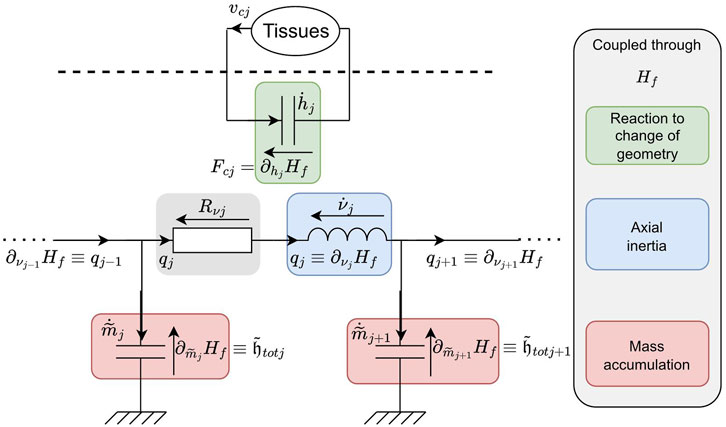
Figure 3. Equivalent circuit representation of a cell of the semi-discrete fluid model. Component laws are coupled through the Hamiltonian and thus depend on the state of the current cell and of the neighbouring sections.

2.2 Vocal fold model

The classical body-cover model of the vocal fods presented in Story and Titze (1994) is used. It consists of a body mass coupled with two cover masses. The port-Hamiltonian formulation has been developed in Encina et al. (2015).

2.2.1 Presentation

The assembly, presented in the left section of Figure 4, comprises the three masses coupled together by four springs and three dampers. Derivation of the port-Hamiltonian formulation of this assembly is recalled here. The body mass $m_b$ describes the displacement of the in-depth vocalis muscle while the lower and upper cover masses $m_l$ and $m_u$ correspond to movements of upstream and downstream parts of the superficial layers (vocal ligament and epithelium). The state of this system, identified by the subscript $t$ for “tissues”, can be chosen as

${\mathit{\alpha }}_t={\left[q_l,q_u,q_b,{\pi }_l,{\pi }_u,{\pi }_b\right]}^{⊺},(20)$

where $q_l$, $q_u$, and $q_b$ are the displacement of the three masses around the equilibrium positions, and ${\pi }_l$, ${\pi }_u$, and ${\pi }_b$ are the momentum of the three masses. From the state, potential energy functions and total potential energy are denoted:

$U_t\left({\mathit{\alpha }}_t\right)=U_l(\underset{≔e_l}{\underbrace{q_l-q_b}})+U_u(\underset{≔e_u}{\underbrace{q_u-q_b}})+U_b(\underset{≔e_b}{\underbrace{q_b}})+U_{lu}(\underset{≔e_{lu}}{\underbrace{q_u-q_l}}).(21)$

Figure 4

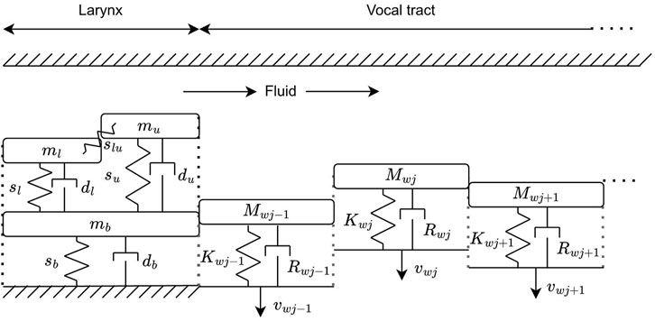
Figure 4. Tissue schematics: body cover model for the vocal fold and mass spring damper systems for vocal tract walls.

The resultant force of the springs on each mass $F_{ri}$ are directly recovered by differentiation with respect to masses displacements:

$F_{ri}={\partial }_{q_i}U\left({\mathit{\alpha }}_t\right).(22)$

The total kinetic energy of the system is computed as

$K_t\left({\mathit{\alpha }}_t\right)=\frac{1}{2}\left(\frac{{\pi }_l^2}{m_l}+\frac{{\pi }_u^2}{m_u}+\frac{{\pi }_b^2}{m_b}\right),(23)$

such that the Hamiltonian is given by

$H_t\left({\mathit{\alpha }}_t\right)=U_t\left({\mathit{\alpha }}_t\right)+K_t\left({\mathit{\alpha }}_t\right).(24)$

The port-Hamiltonian formulation of the dynamics including linear dissipation effects and external interactions is

${\dot{\mathit{\alpha }}}_t=\left(J_t-R_t\right)\nabla H_t\left({\mathit{\alpha }}_t\right)+G_t{\mathbf{u}}_t,(25)$

with

$J_t=\left[\begin{array}{cc}\hfill 0\hfill & \hfill \mathbb{I}\hfill \\ \hfill -\mathbb{I}\hfill & \hfill 0\hfill \end{array}\right],R_t=\left[\begin{array}{cc}\hfill 0\hfill & \hfill 0\hfill \\ \hfill 0\hfill & \hfill R\hfill \end{array}\right],R=\left[\begin{array}{ccc}\hfill r_l\hfill & \hfill 0\hfill & \hfill -r_l\hfill \\ \hfill 0\hfill & \hfill r_u\hfill & \hfill -r_u\hfill \\ \hfill -r_l\hfill & \hfill -r_u\hfill & \hfill r_l+r_u+r_b\hfill \end{array}\right],(26)$

and where dissipation coefficients $r_l$, $r_u$, and $r_b$ are associated with linear dampers. In the numerical experiments, these coefficients are tuned from a single damping ratio $\xi$ as $r_l=2\xi \sqrt{m_l{k}_l}$, $r_u=2\xi \sqrt{m_u{k}_u}$, and $r_b=\xi \sqrt{m_b{k}_b}$. The inputs $u_t=[F_l^{\mathit{ext}},F_u^{\mathit{ext}}]$ are the external forces applied on the lower and upper cover masses, with the associated input matrix:

$G_t={\left[\begin{array}{cccccc}\hfill 0\hfill & \hfill 0\hfill & \hfill 0\hfill & \hfill -1\hfill & \hfill 0\hfill & \hfill 0\hfill \\ \hfill 0\hfill & \hfill 0\hfill & \hfill 0\hfill & \hfill 0\hfill & \hfill -1\hfill & \hfill 0\hfill \end{array}\right]}^{⊺}.(27)$

The power-conjugated output vector ${\mathbf{y}}_t=-G_t^{⊺}\nabla H_t({\mathit{\alpha }}_t)=[v_l,v_u]$ contains the velocities $v_l$ and $v_u$ of the cover masses.

2.2.2 Setting the characteristics of the springs

The above formulations leave us with the choice of potential energy functions $U_i(e_i)$. State-of-the-art lumped models of the vocal folds commonly use nonlinear springs with an added third order term (e.g., Ishizaka and Flanagan, 1972; Story and Titze, 1994,), such that the potential energies, restoring forces, and effective stiffness of individual springs are

$U_i\left(e_i\right)=\frac{1}{2}{k}_i{e}_i^2\left(1+\frac{1}{2}{\left(e_i/e_i^{\mathit{ref}}\right)}^2\right),F_i\left(e_i\right)=k_i{e}_i\left(1+{\left(e_i/e_i^{\mathit{ref}}\right)}^2\right)\text{\hspace{0.17em}and\hspace{0.17em}}{k}^{\text{eff}}\left(e_i\right)=k_i\left(1+3{\left(e_i/e_i^{\mathit{ref}}\right)}^2\right),(28)$

where $e_i^{\mathit{ref}}$ is a reference elongation for the nonlinearity, such that the effective stiffness is multiplied by a factor of four for $e_i=e_i^{\mathit{ref}}$.

2.3 Vocal tract tissue

A better representation of low-frequency resonances of the vocal tract requires the introduction of a model for tissues of the vocal tract. We here consider a simplified local mechanical wall surface impedance $Z_{\mathit{wall}}(\omega )=r_{\mathit{wall}}+j\left(\omega m_{\mathit{wall}}+k_{\mathit{wall}}/\omega \right)$, where $r_{\mathit{wall}}$, $m_{\mathit{wall}}$, and $k_{\mathit{wall}}$ are, respectively, the equivalent unit surface resistance, mass, and stiffness. Their values are adapted from those given in Birkholz et al. (2022). Parameter values for lumped components depicted in the right section of Figure 4 are naturally obtained by integration of their unit surface equivalent on the fluid-structure interface surfaces ($R_{wj}=r_{\mathit{wall}}{L}_0{l}_{dj}$, $M_{wj}=m_{\mathit{wall}}{L}_0{l}_{dj}$, $K_{wj}=k_{\mathit{wall}}{L}_0{l}_{dj}$). The outer wall velocity ${\mathbf{v}}_{\mathbf{w}}$ is an input of the wall dynamical model, such that the overall geometry can still be controlled. The port-Hamiltonian formulation of this model, ready for connection to the fluid model, is presented in Supplementary Appendix SA4.4.

2.4 Assembly

2.4.1 Fluid–tissue connection

In the context of the numerical experiments, the models presented are tested in various configurations. The vocal tract will consist of the fluid model alone, the geometry of which will be controlled by inputs defined in order to produce articulations of different vowels. In the larynx, the fluid model will be connected to the vocal fold model by assuming the continuity of normal velocities and net forces at the fluid–structure interface. Note that several fluid cells may be connected to a single mass of the vocal folds. In this case, connected fluid cells share the same geometrical velocity, and the force received by the vocal fold mass is the result of pressure forces of all fluid cells connected to it. The resulting assembled system can be written as a new port-Hamiltonian system, the state of which is composed of the concatenation of the states of the fluid and the vocal folds.

2.4.2 Glottal closure

In many cases, self-oscillations of the vocal folds include phases of glottal closure and thus contact between the vocal folds. This phenomenon is handled in the modelling by introducing direct coupling between the vocal folds model that is only activated when the vocal folds are detected to be in contact—when the heights $\mathit{h}$ of the fluid elements connected to the vocal fold masses are negative. The implementation is straightforward by adding the compression energy of these springs to the energy of the assembled system without any change in the $J$ matrices. However, the fluid modelling described in Section 2.1 prevents the full closure of the channel, as the reaction force ${\mathbf{F}}_c$ diverges to infinity when $\mathbf{h}$ goes to 0, making the system stiff—which makes time integration difficult.

Mora et al. (2021b) proposed a switching port-Hamiltonian model that disconnects the fluid from the vocal folds when $\mathbf{h}<{ϵ}_h$, effectively taking the stiffness of the fluid layer away from the dynamics of the fold during contact. Considering the anatomical 3D geometry of the glottal channel and the imperfect contact between vocal folds in the human larynx (possibly with glottal leakage), we propose an alternative non-idealised approach to model contact without the need for logical switches checks during the simulation. Considering a given distance threshold $ϵ$, an effective height $h_{\text{eff}}(h)=ϵ+\frac{\alpha }{\pi }+(h-ϵ)\left(1/2+1/\pi \arctan \left(\frac{h-ϵ}{\alpha }\right)\right)$ of the glottal flow channel is introduced, such that $h_{\text{eff}}(h)\sim \max (h,ϵ)$, with $\alpha$ specifying the smooth transition width. The Hamiltonian for the fluid domain (Equation 13) is then modified to account for the effective glottal heights: $\widehat{H}({\mathit{\alpha }}_f=[\mathit{\nu },\tilde{\mathit{m}},\mathit{h}])=H_f(\mathit{\nu },\tilde{\mathit{m}},h_{\text{eff}}(\mathit{h}))$.

Moreover, the discrepancy $c_{\text{eff}}(h)=h-h_{\text{eff}}\ne 0$ can be interpreted as a measure of compression of the vocal fold tissues and used within a modified Hamiltonian for the vocal fold model ${\widehat{H}}_t({\mathit{\alpha }}_t)=H_t({\mathit{\alpha }}_t)+U_{ci}(c_{\text{eff}}(h_i))$, with $U_{ci}(c_{\text{eff}}(h_i))=1/2k_{ci}{c}_{\text{eff}}^2(h_i)\left(1+1/2{\left(c_{\text{eff}}(h_i)/e_{ci}^{\text{ref}}\right)}^2\right)$ to account for the additional stiffness term corresponding to fold interpenetration. Additional linear dissipation is also added to the folds when they are interpenetrating, taking the form of an augmentation of the damping ratio to its critical value ${\xi }_i=1$ when $q_i\le 0$. The effect of parameters $ϵ$, $\alpha$, $k_c$, and $e_{ci}^{\text{ref}}$ will be discussed in the numerical experiments.

3 Numerical experiments

The energy-consistent model established in the previous section as a port-Hamiltonian system is now tested and discussed through a sequence of numerical experiments of increasing complexity. The final experiment simulates the full vocal apparatus exhibiting self-oscillations, where vowel articulation is achieved through geometrical control of the vocal tract.

3.1 General numerical setting and experimental configurations

For time discretisation, a continuous Galerkin time-stepping method is used which preserves a discrete power balance and is unconditionally stable. The method is presented in Chapter 5 of Müller (2021). Second-order polynomials are used for the projection. All simulations are run at a standard audio sampling rate $44100\text{\hspace{0.17em}Hz}$.

General fluid and fold physical parameters are taken as in Mora et al. (2021b) and listed in Table 1. For each numerical configuration, values of configuration-specific parameters are listed in Table 2. Four configurations are studied.

1. The frequency response of the fluid model alone in static configurations is studied. Resonance frequency convergence with respect to spatial discretisation is shown in the simple case of a straight tube. Formant frequencies obtained from the simulation of a geometry configuration corresponding to a single vowel are compared to experimental estimations.

2. Diphthong articulation: the geometry of the fluid model alone is controlled to produce the articulation of diphthongs. A synthetic glottal flow model is used to excite the vocal tract.

3. Isolated larynx: the fluid model is connected to the fold model, exhibiting self-oscillations. As the vocal tract is not modelled, this configuration corresponds to an excised larynx alone.

4. Larynx and vocal tract: the fluid model extends from the glottis to the lips and is connected to the fold model in the larynx. Again, self-oscillations are observed. The geometry of the part of the fluid model corresponding to the vocal tract is forced to produce diphthongs. This experiment yields a full self-oscillating vocal apparatus.

Table 1

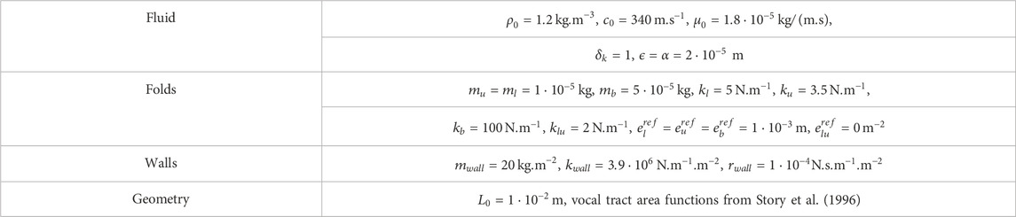
Table 1. General physical constants and parameters.

Table 2

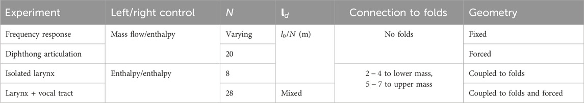
Table 2. Configuration specific parameters.

3.2 Frequency response

In the first experiment, the frequency response of the fluid model in static configurations is studied. Firstly, a straight tube of total length $l_0=17\cdot 10^{-2}$m, homogeneous height $h=1\cdot 10^{-2}$m, and with rigid walls is considered. The model is excited by a mass flow impulse of amplitude $2\cdot 10^{-4}{\text{kg.s}}^{-1}$ on the left end side. On the right end side, a zero total enthalpy is prescribed (no radiation) so that the waveguide should theoretically exhibit resonances at frequencies $f_n=(2n+1)\frac{c_0}{4l_0}$ under acoustic approximations (small-amplitude fluctuations of velocity and enthalpy). As the proposed model is nonlinear, the results of the time-domain simulation are analysed and the frequency response is estimated from the ratio of the spectrum of the right mass flow $q_{\mathit{out}}$ to that of the prescribed impulse of left mass flow $q_{in}$, evidencing as many resonances as the number $N$ of edges. The convergence of resonance frequencies with respect to the spatial discretisation step is studied and shown in Figure 5, with a convergence of order 2.

Figure 5

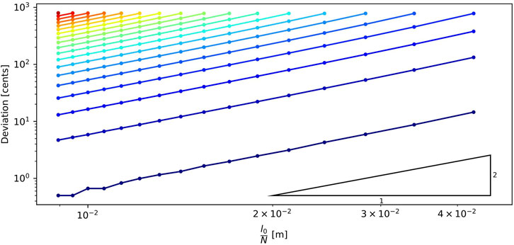
Figure 5. Convergence of resonant frequencies with the number of tracts. Deviation is expressed in cents and is computed as $\text{Deviation}=1200{\log }_2\left(f_{\mathit{sim}}/f_{\mathit{theo}}\right)$, where $f_{\mathit{theo}}$ is the theoretical resonance frequency and $f_{\mathit{sim}}$ that extracted from the simulation. Each line corresponds to a resonance, the first being the lowest on the graph.

Remark 5. Frequency responses are obtained from time-domain simulation of the models. The time discretisation method introduces additional frequency warping. However, in the range of studied frequencies and given the sampling frequency of $44100\text{\hspace{0.17em}Hz}$, it is expected to be of lower impact than the warping due to spatial discretisation. Warping due to spatial discretisation only could be obtained by computations of the eigenvalues of the semi-discrete system linearised around its rest state.

Static vocal tract configurations are now considered. The geometry is set to correspond to a vowel articulation; area functions from Story et al. (1996) are interpolated to produce a set of $N=20$ equidistant cross-section areas from which the values of $\mathbf{h}$ used for the simulation are determined. The total length $l_0$ is set to the vocal tract length corresponding to the simulated vowel. The soft wall model is now used, as well as the radiation condition at the lips. Figure 6 presents the discretised area function for the vowel /ɑ/ and the associated equivalent impedance and mass flow transfer function. Table IV of Story et al. (1996) presents the first three formant frequencies for different vowels, extracted from audio recordings of the individual whose vocal tract geometry was measured. Figure 7 compares these measured values to those obtained from simulations of the model for different vowels. Values obtained from simulation show significant differences with those measured, indicating the need for a better loss model. In particular, and as pointed out in studies such as Fleischer et al. (2015), we observed that the vocal tract wall model shifts up the first formant frequency. The choices made for the fluid domain description in this paper mean that only a part of the fluid domain boundary (corresponding to ${\partial }_{\mathrm{\Omega }}^B$ in Figure 1) corresponds to a fluid–structure interface, reducing the effective area of mobile vocal tract walls. An alternate formulation of the fluid model for arbitrary shape of cross-sections, which would remove this issue, is briefly presented in Supplementary Appendix SA4.5.

Figure 6

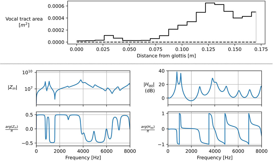
Figure 6. Discretised vocal tract area function for vowel /ɑ/ with $N=20$ (top) and associated equivalent acoustic impedance and mass flow transfer function obtained from time-domain simulation of the model (bottom).

Figure 7

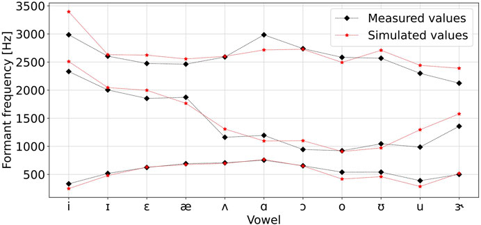
Figure 7. Comparison of the three first formant frequencies of several vowel sounds obtained from simulation of the proposed model with measurement from Story et al. (1996).

3.3 Diphthong articulation

This experiment presents the use of the model as a vocal tract with forced geometry to reproduce co-articulation of diphthongs. The general configuration is similar to the previous one, with a total length $l_0=17\cdot 10^{-2}$m divided into $N=20$ edges. A target sequence of vowels is chosen. From this sequence, a target time trajectory for $\mathbf{h}$ is derived by linear interpolation between individual vowel geometries and smoothed using an averaging filter. The corresponding input velocity to control the model is obtained using a finite difference operator, ensuring that the effective trajectory of $\mathbf{h}$ obtained by simulation is the same as the target trajectory. An example target sequence for diphthong /ɑo/ is given at the top of Figure 8, presenting the wideband spectrogram of the radiated pressure $p_{\mathit{rad}}={\rho }_0{R}_{\mathit{rad}}{q}_{\mathit{rad}}$ for a simulation corresponding to this trajectory and using a synthetic glottal flow model (Klatt & Klatt model, e.g., Doval et al., 2006). The spectrogram exhibits the time evolution of formant frequencies as the geometry is modified.

Figure 8

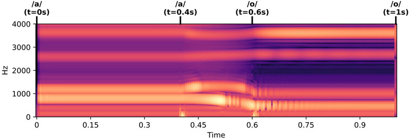
Figure 8. Wideband spectrogram of the radiated pressure for the simulation of the vowel trajectory indicated at the top of the figure. A synthetic glottal flow excitation is used.

Remark 6. The total length $l_0$ of the vocal tract is fixed during the simulation. Indeed, the current model does not allow for length variations of the vocal tract that occur when vowels are articulated.

3.4 Isolated larynx

One of the main objectives of this model is to be able to reproduce self-oscillations of the assembly composed of the laryngeal fluid flow and the vocal folds. We first study a configuration corresponding to an isolated larynx, with no vocal tract model or load. Note that this type of configuration is similar to that presented in Mora et al. (2021b) and can be interpreted as an excised larynx experiment. We use a total of $N=8$ segments for the discretisation of $\mathbf{h}$. Segments $[\mathrm{1,3}]$ are connected to the lower mass of the vocal folds and segments $[\mathrm{4,6}]$ to the upper mass. Segments 0 and 7 are fixed to a height of $h=1\cdot 10^{-2}\text{\hspace{0.17em}m}$. The geometry of the fluid system at rest is defined as

$h_j=\left\{\begin{array}{cc}1\cdot 10^{-2}\text{\hspace{0.17em}m},\hfill & \text{for\hspace{0.17em}}j=0,\hfill \\ 1.8\cdot 10^{-4}\text{\hspace{0.17em}m},\hfill & \text{for\hspace{0.17em}}1\le j\le 3,\hfill \\ 1.79\cdot 10^{-4}\text{\hspace{0.17em}m},\hfill & \text{for\hspace{0.17em}}4\le j\le 6,\hfill \\ 1\cdot 10^{-2}\text{\hspace{0.17em}m},\hfill & \text{for\hspace{0.17em}}j=7,\hfill \end{array}\right.l_{dj}=\left\{\begin{array}{cc}1.5\cdot 10^{-3}\text{\hspace{0.17em}m},\hfill & \text{for\hspace{0.17em}}j=0,\hfill \\ 5\cdot 10^{-4}\text{\hspace{0.17em}m},\hfill & \text{for\hspace{0.17em}}1\le j\le 6,\hfill \\ 1.5\cdot 10^{-3}\text{\hspace{0.17em}m},\hfill & \text{for\hspace{0.17em}}j=7.\hfill \end{array}\right.(29)$

The subglottal total enthalpy is prescribed to be a smoothed step function (as shown in the top axis of Figure 10). An ideal boundary condition is set at the supra-glottal end, enforcing a zero total enthalpy.

3.4.1 Oscillating configuration

Physical parameters from Table 1 are used for simulation, corresponding to case C of Story and Titze (1994). Using their value of $\xi =0.4$ for the damping ratio, the model is unable to oscillate for realistic sub-glottal pressure values. This can be expected as no vocal tract loading is considered in this experiment. However, Story and Titze (1994) mention that estimated values of the damping ratio range from 0.1 to 0.4. Figure 9 presents a cartography of simulation points corresponding to varying values of the sub-glottal pressure step, the approximated value of which is computed from the sub-glottal enthalpy as $P_{\mathit{sub}}=\frac{{\mathfrak{h}}_{\mathit{tot}}}{{\rho }_0}$ and of the damping ratio $\xi$. In the studied range of sub-glottal pressures, oscillations exist only for $\xi \lesssim 0.3$.

Figure 9

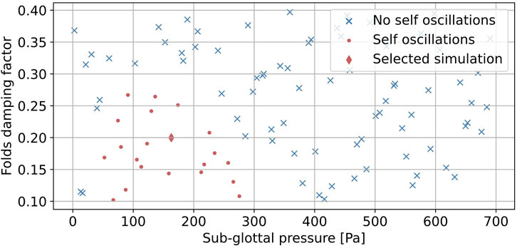
Figure 9. Cartography of oscillating regions as a function of sub-glottal pressure and folds damping factor $\xi$. The diamond marker indicates the simulation studied in following figures.

3.4.2 Signal analysis

Figure 10 shows the distances of the simulated masses to mid-plane and mass flow under the cover masses, obtained for the configuration indicated by a diamond marker in Figure 9. During the first $\sim 0.07$ s, the oscillation builds up to reach a periodic regime, lasting until the input enthalpy is decreased. Glottal closing happens both under the lower and upper superficial masses when their positions are negative. As expected from the high numerical value of $k_b$, the body mass oscillates with a smaller amplitude. The bottom axis of the figure presents a zoom on one period of the oscillation. A clear phase difference is visible between displacements of the lower and upper masses. The model accounts for compressibility and unsteady effects in the fluid. Mass flow signals are similar under both masses, which is expected as the fluid flow in the larynx is, in fact, almost incompressible and stationary. Nonetheless, nonstationary effects related to geometry variations do show a visible effect, such as on the portion of the cycle where the channel is closed under the lower mass but not under the upper one. The mass flow then vanishes under the lower mass but not under the upper mass as its displacement still pushes fluid out of the larynx.

Figure 10

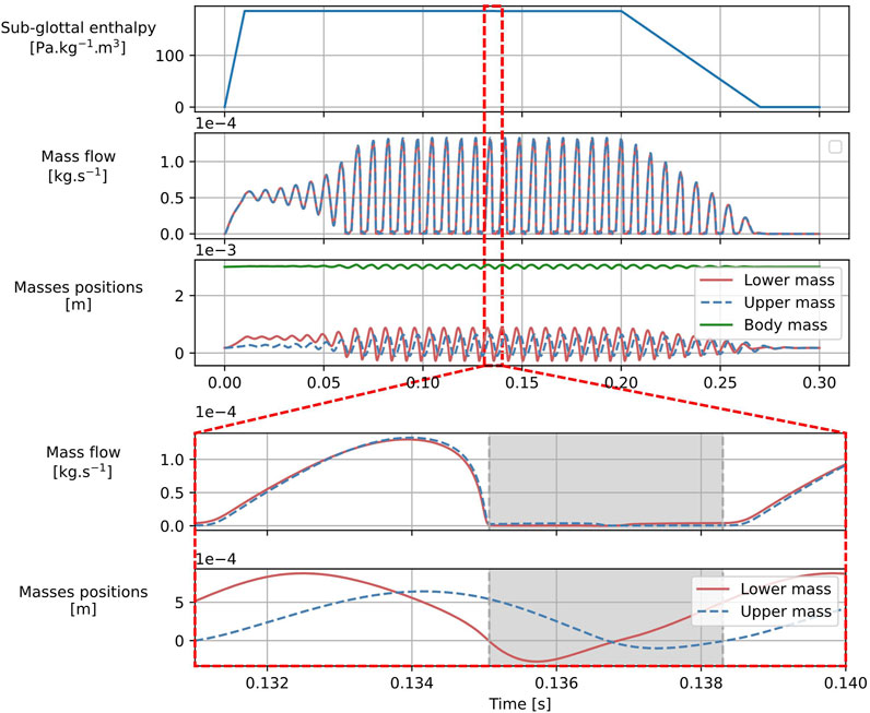
Figure 10. Simulation results in a self-oscillating configuration. Global signals (top) as well as a one-period zoom (bottom) are shown. Masses’ positions are relative to the midplane, and mass flow signals below each of the cover masses are traced. The grey zone in the zoomed signals highlights a closed glottis section of the oscillation cycle.

Time evolution of the terms of the power balance is displayed in Figure 11. The top row presents the variation of the Hamiltonian of both the fluid and tissue systems as well as dissipated power and power exchanged through the boundary at the sub-glottal end of the fluid domain⁵. The power balance is recovered as the sum of these three contributions vanishes (up to numerical precision). This follows from the use of the energy-balanced PDE presented in Equation 8 and of energy-preserving numerical schemes both for space and time discretisation. The bottom row decomposes the dissipated power in three contributions: loss of kinetic energy at the glottal exit (labelled jet), viscous fluid losses, and dissipation within the vocal folds. Analysis of the signals on one period (left column of the figure) provides insightful information on different portions of the cycle:

• During the opened phase (from $\sim 0.1312$s to $\sim 0.1343$s), most of the power provided upstream is used to install a glottal flow whose kinetic energy is largely dissipated at the end of the glottis.

• During the phase of closing of the glottis (from $\sim 0.1343$s to $\sim 0.1351$s), a power transfer from the fluid to the folds builds up. This stems from the Bernoulli effect generating a pressure drop under the lower mass, effectively closing the channel. At the same time, the viscous loss phenomenon in the narrow constriction (scaling with $v_x$) becomes relevant and progressively stops the fluid flow, whereas the kinetic energy loss (scaling with $v_x^2$) vanishes.

• During the closed phase (from $\sim 0.1351$s to $\sim 0.1383$s), fluid dynamics are stopped, and dissipation in the folds is greatly enhanced as the damping factor of cover mass-spring systems is set to 1 during the contact phase.

Figure 11

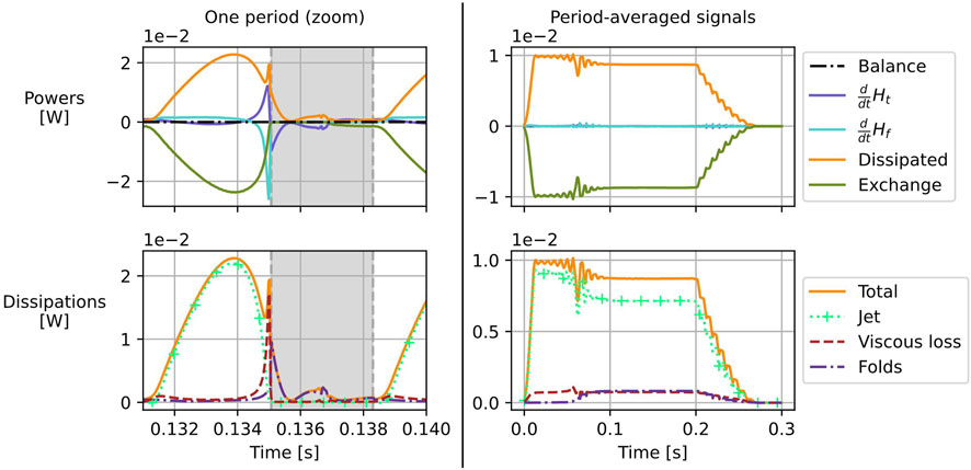
Figure 11. Power signals for the simulation presented in Figure 10. The left column shows the time series of the signals for a single period whereas the right column contains the period-averaged values of these same signals for the full simulation. Dissipated power, power exchanged with the source, and variation of the Hamiltonians of the fluid and fold systems are depicted in the top row with the power balance obtained as the sum of these four contributions. The bottom row separates the dissipated power in its different physical origins: jet dissipation at the larynx output, viscous losses, and dissipation in the folds.

The time-averaged powers are plotted on the right column of Figure 11. After establishing the periodic regime, it is clear that mean variations of the Hamiltonian are null, as expected. Kinetic energy dissipation is the most prominent source of energy loss whereas viscous losses and dissipation in the folds are of the same order of magnitude. From the energy budget of the larynx, the power received from the lower airways is mostly used to install a glottal flow able to produce flow-induced oscillations at the expensive cost of strong kinetic energy losses at the glottal exit. Once the flow is installed, a small extra effort is required to provide the power needed to compensate for viscous losses within the glottis and damping in the tissues.

3.4.3 Numerical experiment on the effect and choice of height regularisation parameters

The parameters $ϵ$ and $\alpha$ specifying the regularisation of the constriction height (Section 2.4.2) do not have a direct physical interpretation, making their values difficult to set. In the following, a choice is made that reduces the numerical stiffness and preserves some important characteristics of the signals. Figure 12 presents snapshots of three simulations corresponding to decreasing values of $ϵ=\alpha =(8\cdot 10^{-5}\text{\hspace{0.17em}m},2\cdot 10^{-5}\text{\hspace{0.17em}m},2\cdot 10^{-6}\text{\hspace{0.17em}m})$, all other parameters being fixed to the same values as for the previous simulation.

Figure 12

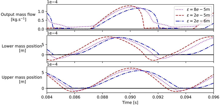
Figure 12. Snapshots of simulations of the larynx alone for different values of the effective height regularisation parameters $ϵ=\alpha \in \{8\cdot 10^{-5},2\cdot 10^{-5},2\cdot 10^{-6}\}$, in meters.

The following can be observed.

• For $ϵ=\alpha =8\cdot 10^{-5}\text{\hspace{0.17em}m}$, both folds interpenetrate during the oscillation cycle as their positions with respect to the midplane goes negative. A significant leak is observed when the channel is closed as the mass flow never reaches 0.

• For $ϵ=\alpha =2\cdot 10^{-5}\text{\hspace{0.17em}m}$, both folds still interpenetrate during the oscillation cycle. However, during the closing of the upper channel, the mass flow is now negligible compared to the amplitude of mass flow oscillations.

• For $ϵ=\alpha =2\cdot 10^{-6}\text{\hspace{0.17em}m}$, the stiff behaviour of the fluid model is seen as it prevents the folds interpenetrating. When the channel is closed, fluid flow is still stopped.

It is preferable to allow folds to interpenetrate as it allows for better control of their behaviour during contact by tuning $k_c$ and ${\eta }_c$, effectively reducing the stiffness of the numerical problem. When the channel is closed, fluid flow should be stopped. Here, the value of $ϵ=\alpha =2\cdot 10^{-5}$ m is used for the simulations as it yields qualitatively good behaviour at channel closing by letting folds interpenetrate and stopping fluid flow. Further studies are necessary to assess the impact of this choice on phonation pressure thresholds and to find an optimal value from comparison with measurements or higher order models.

3.5 Larynx connected to vocal tract

This last experiment focuses on the simulation of the larynx coupled to the vocal tract. This effectively represents a simplified vocal apparatus capable of self-oscillations and articulations. A total of $N=27$ fluid segments are used, with the first seven segments corresponding to the larynx and the remaining 20 representing the vocal tract (Figure 4). Segments 1 to 3 are connected to the lower mass of the vocal folds, and segments 4 to 6 are connected to the upper mass. The lengths of the segments are defined as follows:

$l_{dj}=\left\{\begin{array}{cc}1\cdot 10^{-2}\text{\hspace{0.17em}m},\hfill & \text{for\hspace{0.17em}}j=0,\hfill \\ 5\cdot 10^{-4}\text{\hspace{0.17em}m},\hfill & \text{for\hspace{0.17em}}1\le j\le 6,\hfill \\ \frac{17.46\cdot 10^{-2}}{20}\text{\hspace{0.17em}m},\hfill & \text{for\hspace{0.17em}}7\le j\le 26.\hfill \end{array}\right.(30)$

This configuration reproduces the concatenation of the larynx and vocal tract fluid models used in the previous experiments. The soft wall model is used in the vocal tract, and the boundary condition at the lips is set using the high-pass radiation model. Like the isolated larynx case, the sub-glottal total enthalpy serves as the control input and is set to a smoothed step function. The vocal tract geometry follows the trajectory defined in Figure 8 to produce the diphthong /ɑo/. Initial laryngeal heights are retained from Section 3.4 (see Equation 29), the damping ratio for the vocal folds set to $\xi =0.4$, and other physical parameters are provided in Table 1.

Time-domain results are presented in Figure 13. The top axis of the figure displays the mass flow and cover mass displacement signals over the full simulation duration. Oscillations build up at the start of the simulation, followed by a stable periodic regime, which is then modified by the transition of the vocal tract shape from /ɑ/ to /o/ between 0.4s and 0.6s. After 0.6s, the vocal tract geometry remains fixed, leading to another stable periodic regime. The output mass flow amplitude, shown in grey in the middle row, is significantly altered after the change in vocal tract shape. This change is likely due to the substantial modification in the vocal tract area at the lips, between the wide opening for /ɑ/ and the narrow opening for /o/.

Figure 13

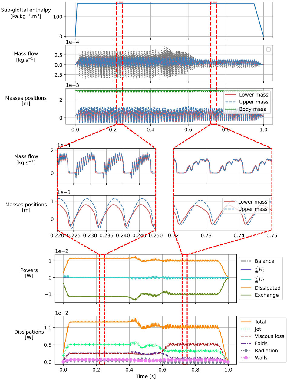
Figure 13. Simulation results for the co-articulation of diphthong /ɑo/ in self-oscillating condition. Signals of mass displacements relative to the midplane and mass flows in the larynx are traced for the full simulation time (top) and two reduced time spans corresponding to stable /ɑ/ and /o/ configurations (middle). Averaged power balance signals and dissipations are also presented (bottom).

The middle axis of the figure depicts zoomed-in views of two stable periodic regimes corresponding to vowels /ɑ/ and /o/. The mass flow signals in the glottis are strongly influenced by the vocal tract, as shown by comparisons of the respective waveforms. In addition, the fundamental frequency is noticeably lower for /o/ (99 Hz) than for /ɑ/ (119 Hz). However, the displacement of the masses is less perturbed by the acoustic coupling with the vocal tract than the mass flow signals.

Averaged power signals are shown at the bottom of the figure, with the averaging filter length set to ten periods of oscillation for configuration /ɑ/. Unfiltered signals, containing high-frequency content (amplified by the vocal tract), are not displayed; however, the global power balance is verified up to machine precision at each time step. The distinct physical origins of dissipated power—jet dissipation at the larynx output, viscous fluid losses, dissipation in the folds, radiated power at the lips, and dissipation within the vocal tract walls—have varying contributions. In particular, viscous fluid losses and fold dissipation are more important here than in cases without a vocal tract (Figure 11). Moreover, the relative contributions of each dissipation mechanism shift substantially after the vocal tract shape modification—notably the increase of the dissipated power related to viscous effects in the glottis and the vocal tract. Further investigation is needed to explain this effect.

4 Discussion and perspectives

This study demonstrates the effectiveness of a quasi-1D port-Hamiltonian model in replicating key characteristics of voice production, ensuring well-posed energy transfer dynamics between fluid, tissues, and human control. The model exhibits self-oscillatory laryngeal behaviours and incorporates a variable-geometry vocal tract. It thus serves as a simple voice synthesizer capable of articulating vowels. This positions the approach as a basis for developing a powerful tool for voice synthesis. This statement is discussed in two parts: firstly, through an analysis of the proposed model, and second, by considering motivated refinements for future model development.

4.1 Simulations of the proposed model

In Section 3, we presented several simulations of the proposed model corresponding to different configurations.

Vocal tract simulations show the evolution of formant frequencies with variations of geometry of the conduit. The incorporation of dissipative effects, such as radiation losses and wall vibrations, proved crucial for obtaining realistic formant bandwidths and frequencies—in line with Fleischer et al. (2015) and Birkholz et al. (2022). Story et al. (1996) provides a set of MRI measurements of vocal tract area functions corresponding to vowel sounds, as well as the corresponding first three formant frequencies extracted from acoustic recordings. Significant error is observed between these measured formant frequencies and our model predictions, which seems related to our choice of vocal tract wall and radiation parameters. The discrepancies observed between these measured formant frequencies and the model predictions—likely stemming from parameter choices related to vocal tract wall damping and radiation losses—highlight the need for further research to refine the modelling of dissipation mechanisms or to optimize these parameters for enhanced realism.

Simulations of the larynx alone and of the complete system show self-oscillations of the vocal folds with constant sub-glottal total enthalpy. We proposed a regularisation procedure to eliminate the unrealistic behaviour of the discrete fluid model at glottal closure. Qualitative analysis of simulation results for different values of the regularisation parameter $ϵ$ emphasises the effects of this procedure. Consequently, the proposed model is suitable for the sound synthesis of voiced sounds with coupling between glottis and vocal tract. It enables vowel articulation during self-oscillation and, theoretically, also consonant articulation, given the model’s capability to handle local closures of the vocal tract. The study of this last point will require the careful design of an appropriate control of the geometry.

The reduced-dimensional approach adopted in this work also proves valuable for exploring the parameter space, particularly in determining oscillation pressure thresholds and pressure-fundamental frequency relationships (Alipour and Scherer, 2007; Ruty et al., 2007). This offers a natural extension of the work presented, allowing comparison with in vivo measurements (in the context of the ANR project AVATARS) or other models. This ability to perform parameter studies is an advantage of the low order fluid models such as that proposed here. Models with two- or three-dimensional flows are more precise but generally too expensive (days of computation for a few oscillation cycles) to perform parameter studies. Voice synthesis based on machine learning is efficient and produces very convincing results. However, any access to the physical variables involved in voice production is lost.

To facilitate future numerical experiments, the development of a fast numerical integration method is of great interest. Indeed, the current in-house iterative solver based on the method presented in Müller (2021), chapter 3 is fully implicit and results in long simulation times (in the order of 10 min of computation time for 1 s of sound). Ongoing research is focused on the development of a fast (explicit or semi-explicit) time-stepping method that satisfies a discrete power balance. Energy quadratisation techniques involving auxiliary variables, as introduced in Shen et al. (2018), have been successfully applied or extended to various problems in musical acoustics (Ducceschi et al., 2023; Bilbao et al., 2023; Castera and Chabassier, 2023; Russo et al., 2024) and show promise for enabling real-time synthesis, which remains one of our primary future objectives.

4.2 Possible refinements for future models

The use of the port-Hamiltonian (pH) framework allows the procedural connection of multiple sub-systems in a power-balanced way. In this study, subsystems for fluid dynamics, tissues in the larynx and vocal tract, and acoustic radiation were considered. Each subsystem can be refined independently without breaking the overall energy balance and passivity, offering significant flexibility for future model improvements. We propose a list of perspectives in this regard.

4.2.1 Fluid model refinements

Use of the PDE presented in 2.1.1 is, to the best of our knowledge, new in the context of vocal apparatus modelling. Unlike Bernoulli-type glottal flow solvers commonly used in the literature, this model accounts for unsteady effects and compressibility, making it suitable for representing both wave propagation in the vocal tract and glottal flow dynamics. The spatial discretisation of this equation using finite differences results in the model presented in Mora et al. (2021b). However, alternative structure-preserving discretisation methods based on a variational formulation, such as partitioned finite elements (Cardoso-Ribeiro et al., 2018; Brugnoli et al., 2020), could also be employed. Specifically, the cross-section area of the fluid domain may be discretised using methods other than piecewise constant approximations. Our intuition is that a smooth laryngeal profile is expected to improve the behaviour of the discrete fluid model during channel closure and may alleviate the need for the regularisation procedure introduced in Section 2.4.2.

A first necessary step to apply these more involved discretisation methods is to include distributed losses directly in the continuous fluid model. In the larynx, viscous friction terms can be derived from a non-homogeneous axial velocity profile on cross-sections, modelled using a boundary layer approach. This is incompatible with the homogeneity assumption (H8) on $v_x$, requiring a relaxation of this hypothesis in future work. A basic possible solution could be to approximate ${\int }_S{v}_x^{2}dS\approx {\left({\int }_S{v}_{x}dS\right)}^2$ in the Hamiltonian (or to consider both the average and the standard deviation of $v_x$ as more detailed degrees of freedom). Additionally, kinetic energy losses due to partial pressure recovery at abrupt changes in cross-section area arise from complex turbulent phenomena. These phenomena cannot be captured well by a 3D-to-1D reduction but may be partially represented by localising an ideal point where airflow separates from the glottal walls. In this study, the separation point is fixed at the exit of the glottis. Future work could incorporate a dynamic separation point, as proposed in Pelorson et al. (1994).

4.2.2 Vocal fold model refinements

The vocal fold model we use is the body-cover model from Story and Titze (1994). Numerous lumped-element vocal fold models, often based on mass-spring assemblies, have been developed over the years (see Erath et al., 2013 for a review). Most of these models are straightforward to implement within the port-Hamiltonian framework and could be used with the fluid model presented here without major difficulty. The proposed framework also allows for the consideration of asymmetric vocal folds, which could be useful for studying pathological configurations (Xue et al., 2010).

Following the earlier discussion around the fluid equations, the use of “aerodynamically smooth” vocal fold models seems particularly promising. However, one of the main challenges of these lumped-element models is the identification of accurate physical parameters. Modal representations derived from the reduction of complex finite element models, as presented in Yokota et al. (2021), may help improve this.

4.2.3 Control issues

Controlling vocal fold parameters based on muscle activations is crucial for achieving realistic pitch modulation and natural vibrato mechanisms in sound synthesis. Integrating control rules, such as those proposed in Titze and Story (2002), into the current framework while maintaining the preservation of energetic properties also represents a promising avenue for future development.

Data availability statement

The original contributions presented in the study are included in the article/Supplementary Material; further inquiries can be directed to the corresponding author.

Author contributions

TR: Conceptualization, Formal Analysis, Investigation, Methodology, Software, Validation, Visualization, Writing – original draft, Writing – review and editing, Data curation. TH: Conceptualization, Funding acquisition, Methodology, Supervision, Writing – original draft, Writing – review and editing, Formal Analysis, Investigation. FS: Conceptualization, Methodology, Supervision, Writing – original draft, Writing – review and editing, Formal Analysis, Investigation, Visualization.

Funding

The author(s) declare that financial support was received for the research and/or publication of this article. This research was funded, in whole or in part, by l’Agence Nationale de la Recherche (ANR), project AVATARS (ANR-22-CE48-0014).

Conflict of interest

The authors declare that the research was conducted in the absence of any commercial or financial relationships that could be construed as a potential conflict of interest.

Generative AI statement

The author(s) declare that no Generative AI was used in the creation of this manuscript.

Publisher’s note

All claims expressed in this article are solely those of the authors and do not necessarily represent those of their affiliated organizations, or those of the publisher, the editors and the reviewers. Any product that may be evaluated in this article, or claim that may be made by its manufacturer, is not guaranteed or endorsed by the publisher.

Supplementary material

The Supplementary Material for this article can be found online at: https://www.frontiersin.org/articles/10.3389/frsip.2025.1525198/full#supplementary-material

Footnotes

¹See Mora et al. (2021a) for port-Hamiltonian formulations of general 3D fluid mechanics

²(H6) directly provides an instantaneous relationship between $\mathbf{w}$, ${\mathbf{v}}_{\mathbf{y}}$, and possibly ${\mathbf{v}}_{\mathbf{x}}$ at the fluid structure interfaces. Elsewhere, values of ${\mathbf{v}}_{\mathbf{y}}$ have no impact on the fluid system presented below and are thus never reconstructed. Refer to Wetzel (2021) for a port-Hamiltonian model that incorporates this transverse component into the Hamiltonian and addresses its effects on the power exchanges at the mobile fluid–structure interfaces

³Consider the fluid at rest state—$\rho (x,t)$ is then a homogeneous quantity on the domain; however, $\mu (x,t)$ is not. In particular, and given the chosen discretisation of $h(x,t)$, $\mu (x,t)$ is not homogeneous on the edges of the dual grid. To correctly represent the rest state, it is then preferable to approximate $\rho (x,t)$ than $\mu (x,t)$.

⁴As a hemilarynx is considered

⁵With the chosen convention, the exchanged power is the power received by the source, meaning that negative values imply a positive power transfer from the source to the system

References

Alipour, F., Berry, D. A., and Titze, I. R. (2000). A finite-element model of vocal-fold vibration. J. Acoust. Soc. Am. 108, 3003–3012. doi:10.1121/1.1324678

PubMed Abstract | CrossRef Full Text | Google Scholar

Alipour, F., and Scherer, R. C. (2007). On pressure-frequency relations in the excised larynx. J. Acoust. Soc. Am. 122, 2296–2305. doi:10.1121/1.2772230

PubMed Abstract | CrossRef Full Text | Google Scholar

Bilbao, S., Webb, C., Wang, Z., and Ducceschi, M. (2023). “Real-time gong synthesis,” in Proceedings of the 26th Conference of Digital audio effects (DAFx-23) (Copenhagen, Denmark).

Google Scholar

Birkholz, P., Hasner, P., and Kurbis, S. (2022). “Acoustic comparison of physical vocal tract models with hard and soft walls,” in IEEE international conference on acoustics, speech and signal processing (ICASSP 2022) (IEEE), 8242–8246. doi:10.1109/ICASSP43922.2022.9746611

CrossRef Full Text | Google Scholar

Brugnoli, A., Cardoso-Ribeiro, F. L., Haine, G., and Kotyczka, P. (2020). Partitioned finite element method for structured discretization with mixed boundary conditions. IFAC-PapersOnLine 53, 7557–7562. doi:10.1016/j.ifacol.2020.12.1351

CrossRef Full Text | Google Scholar

Cardoso-Ribeiro, F. L., Matignon, D., and Lefèvre, L. (2018). A structure-preserving partitioned finite element method for the 2D wave equation. IFAC-PapersOnLine 51, 119–124. doi:10.1016/j.ifacol.2018.06.033

CrossRef Full Text | Google Scholar

Castera, G., and Chabassier, J. (2023). Numerical analysis of quadratized schemes. Application to the simulation of the nonlinear piano string. Tech. Rep. RR-9516. Inria.

Google Scholar

Doval, B., d’Alessandro, C., and Henrich Bernardoni, N. (2006). The spectrum of glottal flow models. Acta Acustica united Acustica 92, 1026–1046.

Google Scholar

Ducceschi, M., Hamilton, M., and Russo, R. (2023). “Simulation of the snare-membrane collision in modal form using the scalar auxiliary variable (SAV) method,” in Proceedings of the forum acusticum 2023. doi:10.61782/fa.2023.0995

CrossRef Full Text | Google Scholar

Encina, M., Yuz, J., Zanartu, M., and Galindo, G. (2015). “Vocal fold modeling through the port-Hamiltonian systems approach,” in 2015 IEEE conference on control applications (CCA) (Sydney, Australia: IEEE), 1558–1563. doi:10.1109/CCA.2015.7320832

CrossRef Full Text | Google Scholar

Erath, B. D., Zañartu, M., Stewart, K. C., Plesniak, M. W., Sommer, D. E., and Peterson, S. D. (2013). A review of lumped-element models of voiced speech. Speech Commun. 55, 667–690. doi:10.1016/j.specom.2013.02.002

CrossRef Full Text | Google Scholar

Flanagan, J. L. (1965). Speech analysis synthesis and perception. Berlin, Heidelberg: Springer Berlin Heidelberg. doi:10.1007/978-3-662-00849-2

CrossRef Full Text | Google Scholar

Fleischer, M., Pinkert, S., Mattheus, W., Mainka, A., and Mürbe, D. (2015). Formant frequencies and bandwidths of the vocal tract transfer function are affected by the mechanical impedance of the vocal tract wall. Biomechanics Model. Mechanobiol. 14, 719–733. doi:10.1007/s10237-014-0632-2

PubMed Abstract | CrossRef Full Text | Google Scholar

Guasch, O., Ternstrom, S., Arnela, M., and Alıas, F. (2013). Unified numerical simulation of the physics of voice: The EUNISON project. The International Society for Computers and Their Applications (ISCA).

Google Scholar

Gunter, H. E. (2003). A mechanical model of vocal-fold collision with high spatial and temporal resolution. J. Acoust. Soc. Am. 113, 994–1000. doi:10.1121/1.1534100

PubMed Abstract | CrossRef Full Text | Google Scholar

Hélie, T., and Silva, F. (2017). “Self-oscillations of a vocal apparatus: a port-Hamiltonian formulation,” in Proceedings of geometric science of information: third international conference (GSI 2017). Editors F. Nielsen,, and F. Barbaresco (Paris, France: Springer International Publishing), 375–383.

CrossRef Full Text | Google Scholar

Ishizaka, K., and Flanagan, J. L. (1972). Synthesis of voiced sounds from a two-mass model of the vocal cords. Bell Syst. Tech. J. 51, 1233–1268. doi:10.1002/j.1538-7305.1972.tb02651.x

CrossRef Full Text | Google Scholar

Kelly, J. L. (1962). “Speech synthesis,” in Proc. Speech communication seminar. Stockholm (Sep. 1962.

Google Scholar

Maeda, S. (1982). A digital simulation method of the vocal-tract system. Speech Commun. 1, 199–229. doi:10.1016/0167-6393(82)90017-6

CrossRef Full Text | Google Scholar

Maschke, B., and van der Schaft, A. (1992). Port-controlled Hamiltonian systems: modelling origins and systemtheoretic properties. IFAC Proc. Vol. 25, 359–365. doi:10.1016/S1474-6670(17)52308-3

CrossRef Full Text | Google Scholar

Mora, L. A., Le Gorrec, Y., Matignon, D., Ramirez, H., and Yuz, J. I. (2021a). On port-Hamiltonian formulations of 3-dimensional compressible Newtonian fluids. Phys. Fluids 33, 117117. doi:10.1063/5.0067784

CrossRef Full Text | Google Scholar

Mora, L. A., Ramirez, H., Yuz, J. I., Le Gorec, Y., and Zañartu, M. (2021b). Energy-based fluid–structure model of the vocal folds. IMA J. Math. Control Inf. 38, 466–492. doi:10.1093/imamci/dnaa031

PubMed Abstract | CrossRef Full Text | Google Scholar

Mora, L. A., Yuz, J. I., Ramirez, H., and Gorrec, Y. L. (2018). A port-Hamiltonian fluid-structure interaction model for the vocal folds this work was supported by CONICYT-PFCHA/2017-21170472, and AC3E CONICYT-basal project FB-0008. IFAC-PapersOnLine 51, 62–67. doi:10.1016/j.ifacol.2018.06.016

CrossRef Full Text | Google Scholar

Müller, R. (2021). Time-continuous power-balanced simulation of nonlinear audio circuits: realtime processing framework and aliasing rejection. Sorbonne Université: Ph.D. thesis.

Google Scholar

Olver, P. J. (1986). Applications of lie groups to differential equations, 107. New York, NY: Graduate Texts in Mathematics. doi:10.1007/978-1-4684-0274-2

CrossRef Full Text | Google Scholar

Pelorson, X., Hirschberg, A., Van Hassel, R. R., Wijnands, A. P. J., and Auregan, Y. (1994). Theoretical and experimental study of quasisteady-flow separation within the glottis during phonation. Application to a modified two-mass model. J. Acoust. Soc. Am. 96, 3416–3431. doi:10.1121/1.411449

CrossRef Full Text | Google Scholar

Risse, T., Hélie, T., Silva, F., and Falaize, A. (2024). Minimal port-Hamiltonian modeling of voice production: choices of fluid flow hypotheses, resulting structure and comparison. IFAC-PapersOnLine 58, 238–243. doi:10.1016/j.ifacol.2024.08.287

CrossRef Full Text | Google Scholar

Russo, R., Bilbao, S., and Ducceschi, M. (2024). Scalar auxiliary variable techniques for nonlinear transverse string vibration. IFAC-PapersOnLine 58, 160–165. doi:10.1016/j.ifacol.2024.08.274

CrossRef Full Text | Google Scholar

Ruty, N., Pelorson, X., Van Hirtum, A., Lopez-Arteaga, I., and Hirschberg, A. (2007). An in vitro setup to test the relevance and the accuracy of low-order vocal folds models. J. Acoust. Soc. Am. 121, 479–490. doi:10.1121/1.2384846

PubMed Abstract | CrossRef Full Text | Google Scholar

Shen, J., Xu, J., and Yang, J. (2018). The scalar auxiliary variable (SAV) approach for gradient flows. J. Comput. Phys. 353, 407–416. doi:10.1016/j.jcp.2017.10.021

CrossRef Full Text | Google Scholar

Stevens, K. N. (1971). Airflow and turbulence noise for fricative and stop consonants: static considerations. J. Acoust. Soc. Am. 50, 1180–1192. doi:10.1121/1.1912751

CrossRef Full Text | Google Scholar

Story, B. H., and Titze, I. R. (1994). Voice simulation with a body-cover model of the vocal folds. J. Acoust. Soc. Am. 97, 1249–1260. doi:10.1121/1.412234

PubMed Abstract | CrossRef Full Text | Google Scholar

Story, B. H., Titze, I. R., and Hoffman, E. A. (1996). Vocal tract area functions from magnetic resonance imaging. J. Acoust. Soc. Am. 100, 537–554. doi:10.1121/1.415960

PubMed Abstract | CrossRef Full Text | Google Scholar

Titze, I. R., and Story, B. H. (2002). Rules for controlling low-dimensional vocal fold models with muscle activation. J. Acoust. Soc. Am. 112, 1064–1076. doi:10.1121/1.1496080

PubMed Abstract | CrossRef Full Text | Google Scholar

Trenchant, V., Ramirez, H., Le Gorrec, Y., and Kotyczka, P. (2018). Finite differences on staggered grids preserving the port-Hamiltonian structure with application to an acoustic duct. J. Comput. Phys. 373, 673–697. doi:10.1016/j.jcp.2018.06.051

CrossRef Full Text | Google Scholar

Valášek, J. (2021). Numerical simulation of fluid-structure-acoustic interaction in human phonation. Czech Technical University. Ph.D. thesis.

Google Scholar

Wetzel, V. (2021). Lumped power-balanced modelling and simulation of the vocal apparatus: a fluid-structure interaction approach. Sorbonne Université: Ph.D. thesis.

Google Scholar

Xue, Q., Mittal, R., Zheng, X., and Bielamowicz, S. (2010). A computational study of the effect of vocal-fold asymmetry on phonation. J. Acoust. Soc. Am. 128, 818–827. doi:10.1121/1.3458839

PubMed Abstract | CrossRef Full Text | Google Scholar

Yokota, K., Ishikawa, S., Takezaki, K., Koba, Y., and Kijimoto, S. (2021). Numerical analysis and physical consideration of vocal fold vibration by modal analysis. J. Sound Vib. 514, 116442. doi:10.1016/j.jsv.2021.116442

CrossRef Full Text | Google Scholar

Zhang, Z. (2015). Regulation of glottal closure and airflow in a three-dimensional phonation model: implications for vocal intensity control. J. Acoust. Soc. Am. 137, 898–910. doi:10.1121/1.4906272

PubMed Abstract | CrossRef Full Text | Google Scholar