Reinforcement learning, rule-based, or generative AI: a comparison of model-free Wi-Fi slicing approaches

Resource allocation techniques are key to providing Quality-of-Service guarantees. Wi-Fi standards define features enabling the allocation of radio resources across time, frequency, and link band. However, radio resource slicing, as implemented in 5G cellular networks, is not native to Wi-Fi. A few reinforcement learning (RL) approaches have been proposed for Wi-Fi resource allocation and demonstrated using analytical models where the reward gradient with respect to the model parameters is accessible—i.e., with a differentiable Wi-Fi network model. In this work, we implement—and release under an Apache 2.0 license—a state-of-the-art, state-augmented constrained optimization method using a policy-gradient RL algorithm that does not require a differentiable model, to assess model-free RL-based slicing for Wi-Fi frequency resource allocation. We compare this with six model-free baselines: three RL algorithms (REINFORCE, A2C, PPO), two rule-based heuristics (Uniform, Proportional), and a generative AI policy using a commercial foundational Large Language Model (LLM). For rapid RL training, a simple, non-differentiable network model was used. To evaluate the policies, we use an ns-3-based Wi-Fi 6 simulator with a slice-aware MAC. Evaluations were conducted in two traffic scenarios: A) a periodic pattern with one constant low-throughput slice and two high-throughput slices toggled sequentially, and B) a random walk scenario for realism. Results show that, on average—in terms of the trade-off between total throughput and a packet-latency-based metric—the uniform split and LLM-based policy perform best, appearing on the Pareto front in both scenarios. The proportional policy only appears on the front in the periodic case. Our state-augmented constrained approach based on REINFORCE (SAC-RE) is on the second Pareto front for the random walk case, outperforming vanilla REINFORCE. In the periodic scenario, vanilla REINFORCE achieves better throughput—with a latency trade-off—and is co-located with SAC-RE on the second front. Interestingly, the LLM-based policy—neither trained nor fine-tuned on any custom data—consistently appears on the first Pareto front, offering higher objective values at some latency cost. Unlike uniform slicing, its behavior is dynamically adjustable via prompt engineering.

1 Introduction

Network slicing is a technique used to guarantee Quality-of-Service (QoS) by allocating resources in a way that allows the network to meet traffic flow requirements. Slicing can be implemented in wireless networks through various mechanisms that leverage the features available in a given technology domain. The CSMA channel access mechanism of Wi-Fi was designed as a solution that provides fairness to all devices, albeit with no guarantees. Slicing allows for the design of a network that trades off this fairness but can provide guarantees in Quality of Service if required. A challenge that arises is that if the slicing policy is not well optimized, it can lead to inefficiencies and waste of resources.

In cellular networks, such as 5G, the 3GPP standards define the capability to schedule channel communication resources in both time and frequency. This capability has been exploited to implement slicing of the radio channel (Zhang, 2019).

Wi-Fi, on the other hand, has employed a contention-based approach for channel access since its inception, making it more challenging to guarantee QoS. Over time, Wi-Fi standards, defined by the IEEE 802.11 working group, have evolved to offer greater control over channel access, enabling the deployment of centrally managed networks via an Access Point (AP), where deterministic policies can be implemented. However, limited work exists on the implementation of slicing concepts in Wi-Fi. Since Wi-Fi 6, frequency resources can be allocated by the AP to different users. In contrast to 5G cellular standards—where Physical Resource Blocks (PRBs) are allocated in both time and frequency domains—the AP can only allocate the resources of within a Physical Layer Protocol Unit (PPDU) once it starts a transmission opportunity (TXOP) after gaining channel access; see Figure 1.

Figure 1

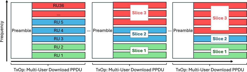
Figure 1. Slicing of Wi-Fi OFDMA frequency resources. Since Wi-Fi 6, an AP can centrally schedule multi-user downlink and uplink transmissions. After acquiring a transmission opportunity (TxOp), the AP can individually assign resource units (RUs) to different client stations (STAs) within a multi-user Physical Protocol Data Unit (PPDU). In this work, we dynamically allocate multiple RUs to create slices in the frequency domain.

Zangooei et al. (2023), Yang et al. (2024), and Liu et al. (2020) are examples of Artificial Intelligence (AI) approaches based on Reinforcement Learning (RL) for optimizing resource allocation.

Work incorporating QoS constraints—such as Yang et al. (2024) and Liu et al. (2020) — typically focuses on creating a single objective function by combining multiple constraints and the main objective into a weighted sum. Liu et al. (2021) explore constraint-aware optimization through Lagrangian primal-dual methods. Calvo-Fullana et al. (2023) proposed an improvement to these methods using the concept of state-augmented RL, where the values of the Lagrangian multipliers are fed as input to the policy. This enables the learning of different behaviors depending on the current system state.

The state-augmented approach has been adopted by NaderiAlizadeh et al. (2022) and Uslu et al. (2024) for radio resource allocation of power transmission levels and frequency resources, respectively. Their work applied state-augmented RL using gradient-based direct optimization, which requires computing the gradient of the Lagrangian w.r.t. the policy parameters—i.e., a differentiable model of the system. However, this limits applicability in real systems or simulation environments such as ns-3 (Henderson et al., 2008), where analytical gradients are not available.

Model-free RL approaches, such as policy-gradient Sutton and Barto (1998) methods, estimate the gradients via sampling and therefore do not require a differentiable model of the system.

In this work, we evaluate multiple model-free approaches (see Figure 2), including a proposed adaptation of the state-augmented method from Calvo-Fullana et al. (2023) to the problem of radio frequency resource slicing, as in Uslu et al. (2024).

Figure 2

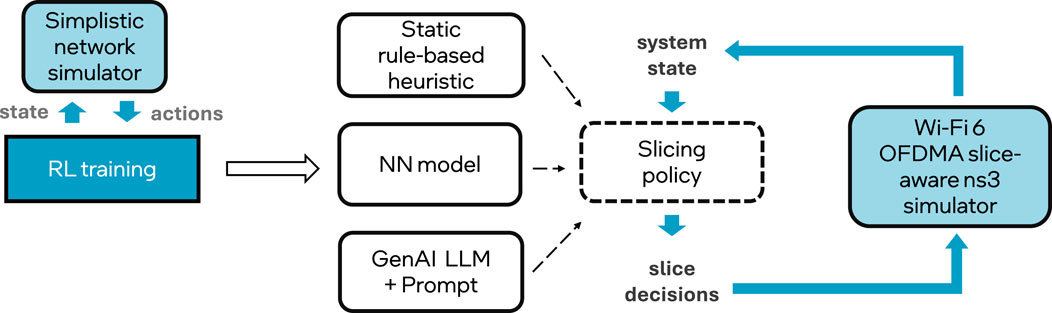
Figure 2. General methodology: RL-based policies are first trained using a simple network simulator. These policies, together with other rule-based and GenAI based policies are evaluated with a ns-3 Wi-Fi simulator.

Alongside other RL and rule-based policies, we also evaluate a Generative AI (GenAI) approach using a Large Language Model (LLM) for RL. In this case, a commercial off-the-shelf (COTS) foundational LLM is used to make slicing decisions. LLMs have demonstrated wide applicability due to their emergent properties developed through training on vast amounts of data. Peng et al. (2023) propose using LLMs as RL policies, offering a natural language interface to specify decisions. Zhou and Small (2021) apply LLMs to learn policies tailored to specific tasks.

2 Network slicing in Wi-Fi

2.1 Wi-Fi radio resource allocation features

Wi-Fi provides some alternatives for slicing the communication channel between different users.

The simplest approach is to separate different flows across different frequency bands or channels—for example, assigning three different flows to the 2.4 GHz, 5 GHz, and 6 GHz bands, respectively. However, this method is typically statically configured a priori and can be inefficient and prone to Quality-of-Service (QoS) degradation due to dynamic channel fluctuations. Furthermore, it is only feasible in multi-radio devices supporting multiple frequency bands.

At a more granular level, since Wi-Fi 6 it is possible to dynamically assign different bandwidths to different flows by splitting a single channel into multiple Resource Units (RUs) in a multi-user PPDU, thereby distributing the available spectrum more efficiently. For example, a 20 MHz channel can be divided into nine RUs, each 2 MHz wide. The decision regarding the number and size of RUs in both downlink and uplink transmissions is dynamically made by the Wi-Fi Access Point (AP). Since Wi-Fi 7, this includes support for aggregating multiple RUs for a single user.

In addition to frequency-domain slicing (Uslu et al., 2024), traffic flows can also be isolated in the time domain. Candell et al. (2022) demonstrated an implementation of the TSN standard for time-aware scheduling (802.1Qbv) in Wi-Fi. Time-domain allocation must also be centrally managed by the AP. It is important to note that, unlike cellular technologies defined by 3GPP, Wi-Fi does not incorporate the concept of Physical Resource Blocks (PRBs), which enable simultaneous allocation in both time and frequency domains. 3GPP cellular networks have always used a centralized scheduling mechanism, allowing for precise allocation of time slots and frequency bands to different users as part of the protocol. Wi-Fi networks, on the other hand, have been based on a decentralized, contention-based access method. Recently, in Wi-Fi 6, the OFDMA scheduling mechanism was introduced, allowing for the assignment of frequency resources within a PPDU. This solution is not as flexible as the 3GPP approach. In Wi-Fi, time-based resource allocation must be done across multiple PPDUs, thus combining it with the decentralized CSMA mechanism for resource contention. To eliminate the contention overhead, a centrally managed Wi-Fi network is assumed for the proposed Wi-Fi radio slicing; that is, all client devices are centrally managed by the AP using OFDMA. Under this assumption, most of the contention overhead due to channel access is eliminated.

In this work, we explore dynamic slicing of Wi-Fi frequency resources—i.e., at each transmission opportunity, the AP decides how many frequency resources to allocate to each of the required slices.

The modulation constellation is determined according to the Wi-Fi standard and is dynamically adjusted based on the available bandwidth of the allocated RUs. The network is configured to use a channel bandwidth of 80 MHz, and the transmission power is set at 20 dBm. The propagation model used is the IEEE 802.11 D channel model. Other potential physical layer features that were not explored in our study include: a) spatial streams using MIMO, as we used a single antenna for both transmission and reception; and b) preamble puncturing, which was not explored.

2.2 Problem formulation

We formulate the slicing problem for Wi-Fi OFDMA frequency resources as a constrained optimization problem:

The goal is to find a slicing decision policy $\pi$ that takes an action $a_t$ based on the system state $s_t$: $\pi (s_t)\to a_t$ that maximizes the expected value of a main objective function $r(s_t,a_t)$, which is here defined as the total amount of bytes received, and which is a function of the system state $s_t$ and the slicing decision $a_t$ at each time step $t\in T$. At the same time, the slicing policy should try to fulfill a set of $J$ constraints defined by a list of inequalities $e_j(s_t,a_t)\le c_j$, where $e_j(s_t,a_t)$ are the constraint functions, and $c_j$ are the constraint specifications. The formal formulation is shown in Equation 1:

$\begin{array}{c}\hfill \underset{\pi }{\max }\underset{T\to \infty }{\lim }{\mathbb{E}}_{s,a\sim \pi }\left[\frac{1}{T}{\displaystyle \sum _{t=0}^T}r(s_t,a_t)\right]\\ \hfill \text{s.t.}\underset{T\to \infty }{\lim }{\mathbb{E}}_{s,a\sim \pi }\left[\frac{1}{T}{\displaystyle \sum _{t=0}^T}{e}_j(s_t,a_t)\right]\le c_j,j=\mathrm{1,2},\dots ,J\end{array}(1)$

In this work, we define the system state $s$ as a vector $s\in {\mathbb{N}}^{H\times N}$. This vector represents the traffic demand in terms of number of packets ready to be transmitted at each slice (with a total of $N$ slices) for the last last $H$ steps.

The policy action $a$ correspond to the slicing decisions, and is defined as a vector $a\in {\mathbb{R}}^N$, such that ${\sum }_{i}a[i]=1$, i.e., it defines what proportion of resources, in this case Wi-Fi RUs, are assigned to each slice $i$ at each time step $t$. In order to enable the finest granularity possible, we select the smallest possible bandwidth for all RUs, and then aggregate them according to the slicing decision. In contrast to a real Wi-Fi implementation, where the bandwidths of the aggregated RUs would be combined for better efficiency, our simulation-based evaluation bundles multiple individual RUs of the same smallest bandwidth. The proposed allocation of multiple RUs for different users is already supported in the Wi-Fi 7 standard (802.11be).

The underlying system dynamics are treated here as a black box, as the explicit modeling of state transitions in the Wi-Fi network is infeasible. This means that while we do not specify an explicit transition model in our objective function, we implicitly rely on the system’s ability to learn these transitions through interaction with the environment. In addition, the problem formulation makes no assumption about the stationarity of the transitions. Thus, only solutions applying dynamic adaptation mechanisms would be effective in a non-stationary environment.

As a constraint, we define a metric based on the average latency of the received packets. The metric adds the individual latencies of each packet as measured from the time of transmission until the time of reception at the MAC layers. For each packet that was not received at all, e.g., because no resource was allocated for the corresponding slice, we include a penalty factor of 100. This penalty is included in this metric to avoid encouraging seemingly low average latency solutions that in reality are filling the transmission queues.

2.3 Solution approaches

Several optimization approaches can be applied to solve Equation 1. The works of Uslu et al. (2024) and NaderiAlizadeh et al. (2022) represent two state-of-the-art RL-based methods that address a closely related problem to slicing wireless communication resources. Both approaches apply the concept of state-augmentation proposed by Calvo-Fullana et al. (2023) to enable multi-modal solutions, where the system may have more than one optimal operating mode. However, these methods have been applied using a differentiable model of the system in order to guide the learning of the policy as dictated by the gradient of the Lagrangian formulation of the optimization problem.

In this work, we explore the implementation of state-augmentation using a policy-gradient, model-free RL approach, i.e., the system does not need to be a differentiable system model. Policy-gradient methods estimate the gradient of the objective function w.r.t. the policy parameters through sampling. While this approach is less sample-efficient and typically results in slower learning, it has the advantage of being applicable directly to real world systems or high-fidelity simulators such as ns-3. On the other hand, verifying the convergence of policy gradient methods in complex environments such as Wi-Fi slicing poses significant challenges due to non-stationarity, high dimensionality, delayed rewards, and the risk of local optima. These environments require algorithms capable of handling dynamic conditions and vast state-action spaces while ensuring consistent policy improvement. Addressing these theoretical challenges is crucial for effectively deploying reinforcement learning solutions in real-world applications like Wi-Fi slicing.

We also evaluate other common policy-gradient RL methods, including the REINFORCE algorithm, along with simple rule-based heuristics and a policy based on a recent large language model. Figure 3 illustrates these approaches in a Venn-diagram, comparing the methods evaluated in this work with the closest related state-of-the-art.

Figure 3

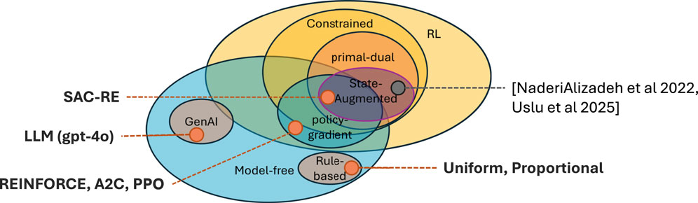
Figure 3. Classification of the approaches evaluated and of the closest related work.

In the next subsection, we describe each of the evaluated approaches in more detail.

2.3.1 Policy-gradient based RL approaches

We evaluate three commonly adopted policy-gradient based RL approaches:

2.3.1.1 REINFORCE algorithm

This method, originally proposed in Williams (1992) and summarized in Algorithm 1, consists of two main phases: a) a sampling phase, where a full episode is executed using the current policy $\pi$ to collect $T$ samples of the system state $s$, the selected action $a$, and corresponding system rewards $r$; and b) an evaluation phase, where a loss is computed based on the negative log-probability of the sampled actions, scaled by the observed rewards. The evaluation phase encourages updates to the policy parameters such that unlikely decisions with high positive rewards become more probable, while decisions that resulted in negative rewards become less likely.

Algorithm 1.REINFORCE algorithm - Williams (1992).

Require: A differentiable policy parameterization $\pi (a|s,\theta )$

Require: Parameters: learning step size $\alpha >0$, reward discount factor $0\le \gamma \le 1$, total episode steps $T\in \mathbb{N}$

1: Initialize policy parameters: $\theta \in {\mathbb{R}}^d$

2: for each episode do

3:  Generate: $s_0,a_0,r_1,\dots ,s_{T-1},a_{T-1},r_T,$ following $\pi (\cdot |\cdot ,\theta )$

4:  for each episode step $t=0,\dots ,T-1$ do

5:   Compute discounted returns: $G\leftarrow {\sum }_{k=t+1}^T{\gamma }^{k-t-1}{r}_k$

6:   Update policy parameters: $\theta \leftarrow \theta +\alpha {\gamma }^{t}G\nabla \ln \pi (a_t|s_t,\theta )$

7:  end for

8: end for

9: return $s_1,s_2,\dots ,s_n$

2.3.1.2 Synchronous advantage Actor-critic (A2C)

One of the main challenges of RE, is selecting an appropriate baseline to determine whether the observed reward should be interpreted as positive or negative. The A2C approach - a synchronous variant of Mnih et al. (2016) - implements a value-based model (the critic) to estimate this baseline and uses the difference between the actual reward and the predicted baseline, known as the advantage, in the loss function. We use the Python implementation provided by Stable-Baselines3 (2025b) for this algorithm. The n_step hyperparameter was set to match the update rate of the other RL algorithms. Other hyper-parameters used the default values.

2.3.1.3 Proximal policy optimization

This approach (Schulman et al., 2017), uses a clipped surrogate loss within a trust region to prevent drastic updates to the policy parameters during training. We use the Python implementation provided by Stable-Baselines3 (2025a) for this algorithm. Again, the n_step hyperparameter was set to match the update rate of the other RL algorithms. Other hyper-parameters used the default values.

2.3.2 Policy-gradient based, state-augmented constrained RL

We implemented a state-augmented implementation of the REINFORCE algorithm. In the remainder of this paper, we refer to this implementation as SAC-RE. Below, we describe the approach and model in detail.

2.3.2.1 State-augmented constrained REINFORCE

Calvo-Fullana et al. (2023) introduced the concept of state-augmentation for constrained reinforcement learning. The core idea is to make the policy model ${\pi }_{\theta }$ a function not only of the system state $s_t$, but also of the Lagrangian multipliers: ${\pi }_{\theta }(s_t,{\lambda }_{j,t})\to a_t$. The Lagrangian multipliers ${\lambda }_{j,t}$ where $j$ denotes the index of the associated constraint, are then used to integrate the $J$ constraints of the problem into a single objective function $r_{\lambda }$:

$r_{\lambda }\left(s_t,a_t\right)=r(s_t,a_t)+{\displaystyle \sum _{j=1}^J}{\lambda }_{j,t}\left(e_j(s_t,a_t)-c_j\right)$

where $r(s_t,a_t)$ is the original reward, $e_j(s_t,a_t)$ is the jth constraint cost signal, and $c_j$ is the associated constraint threshold.

By doing so, the policy can learn different behaviors depending on the current situation or mode, thereby enabling the learning of optimal solutions under varying circumstances.

While REINFORCE, A2C, and PPO struggle to adapt swiftly to abrupt traffic changes due to their update strategies that rely on episodic or incremental updates, the state-augmented approach with Lagrangian multipliers can enhance them. This modification allows for dynamic adjustment and improved responsiveness as soon as a constraint is violated, offering better adaptability in fast-changing environments compared to the slower traditional methods. The Lagrangian formulation of the reward objective allows to dynamically adjust how much importance (or weight) is given to each objective based on how well constraints are being met during learning. Instead of using fixed weights for each objective, the RL algorithm modifies these weights as necessary, aiming to find a solution that minimizes constraint violations. This dynamic adjustment introduces some uncertainty because the specific tradeoff between objectives depends on how the neural network was initialized and trained.

The state-augmented approach defines a training algorithm for the policy, which can incorporate different reinforcement learning methods, and an inference algorithm, that updates the Lagrangian multipliers at runtime.

Algorithm 2.State-augmented training algorithm - Calvo-Fullana et al. (2023).

1: Sample $(s_t,{\lambda }_{j,t})$ from augmented space $S\times \mathrm{\Lambda }$

2: Construct augmented rewards $r_{\lambda }(s_t,a_t)=r(s_t,a_t)+{\sum }_{j=1}^J{\lambda }_{j,t}(e_j(s_t,a_t)-c_j)$

3: Use an RL algorithm to obtain policy $\theta =\arg {\max }_{\theta \in {\mathbb{R}}^d}{\lim }_{T\to \infty }{\mathbb{E}}_{s,a\sim {\pi }_{\theta }}\left[\frac{1}{T}{\sum }_{t=0}^T{r}_{\lambda }(s_t,a_t)\right]$

Algorithm 3.State-augmented inference algorithm - Calvo-Fullana et al. (2023).

Require: Policy $\pi (\cdot |\cdot ,\theta )$, step ${\eta }_{\lambda }$, requirements $c_j$, epoch $T_0$

1: Initialize: Given initial state $s_0$, dual variables ${\lambda }_{j,0}=0$

2: for k = 0,1, … ,K do

3:  Rollout $T_0$ steps with actions $a_t\sim \pi (s_t,{\lambda }_{j=1,k},\dots ,{\lambda }_{j=J,k})$

4:  Update dual variables ${\lambda }_{j,k+1}={\left[{\lambda }_{j,k}-\frac{{\eta }_{\lambda }}{T_0}{\sum }_{t=k{T}_0}^{(k+1)T_0-1}(e_j(s_t,a_t)-c_j)\right]}_{+}$

5: end for

We implemented Step 3 of the State-augmented Training algorithm (Algorithm 2) using the REINFORCE algorithm (Algorithm 1). The inference time algorithm (Algorithm 3) was implemented as originally proposed. For REINFORCE, we adopted a mean baseline - i.e., we subtracted the mean of the episode’s rewards from each observed reward.

The slicing policy model $\pi$ is parameterized by the weights $\theta$ of a multi-layer perceptron (MLP) composed of three linear layers, each followed by a leaky ReLU activation function. The number of inputs corresponds to the number of system state signals multiplied by a factor $H$, as the network receives not only the current system state but also the previous $H$ states. The second linear layer has dimensions $128\times 128$, and the final linear layer has dimensions $128\times N$, where $N$ is the number of slices.

The output of the neural network is used as the set of alpha parameters for a Dirichlet distribution. The Dirichlet distribution parameterizes a probability distribution over components that sum to one, making it suitable for representing resource slicing decisions. Depending on the alpha values, the distribution may favor uniform splits, skewed allocations, or evenly distributed probabilities across possible combinations. A key benefit of using the Dirichlet distribution is that it encourages exploration of diverse slicing combinations - since the model predicts a probability distribution rather than a fixed decision. A deterministic approach using a Softmax function would produce more precise, single-point predictions for resource allocation. While this might simplify decision-making and reduce computational complexity, it could also lead to less robust performance under varying network conditions because it does not inherently capture uncertainty or variability in the same way that a Dirichlet-based probabilistic model does. In our experiments, the alpha parameters of the Dirichlet distribution were constrained to values between 1 and 10,000, allowing the distribution to be flat or moderately peaked, but avoiding excessively sharp outputs.

We used the Adam optimizer (Kingma and Ba, 2015) to update the neural network parameters, with a learning rate of $\alpha =0.0001$.

The source code of the SAC-RE implementation is publicly available in Rosales (2025) under the Apache 2.0 License.

2.3.3 Rule-based approaches

Typical baselines for comparing RL approaches rely on static heuristics, which aim to balance multiple objectives and constraints using simple, rule-based strategies that require no training.

2.3.3.1 Uniform heuristic

This heuristic evenly divides the available resources among all slices. For example, if three slices are defined, it always produces a split of $a=[0.33,0.33,0.33]$. While this approach provides a basic level of fairness - regardless of scenario complexity - it can be inefficient and lead to resource under utilization in dynamic or asymmetric traffic conditions.

$a[i]=\frac{1}{N}(2)$

where $a[i]$ is the allocated amount of resources for slice $i$, $N$ is the total number of slices.

2.3.3.2 Proportional heuristic

This heuristics determines the slicing decision based on a signal of interest - such as current traffic demand - and allocates resources to each slice in proportion to its share of that signal.

$a[i]=\frac{w_i}{{\sum }_{k=1}^N{w}_k}(3)$

where $a[i]$ is the allocated amount of resources for slice $i$, $w_i$ is the signal of interest of slice $i$, and $N$ is the total number of slices.

2.3.4 Generative AI approach

2.3.4.1 LLM heuristic

Large Language Models (LLMs) have recently gained significant attention due to their emergent capabilities. An LLM is a neural network trained at scale in a self-supervised manner on vast amounts of text data, with the goal of predicting the most likely next word in a sequence. These models can contain billions of parameters, and despite their relatively simple training objective, they are capable of generating highly plausible and contextually appropriate text across a wide range of domains.

Recently, LLMs have begun to be integrated as decision-making components within RL frameworks, such as Peng et al. (2023). In this work, we evaluate the performance of a foundational LLM as a slicing policy - i.e., an LLM that has not been fine-tuned or optimized for a specific task, but rather used originally pre-trained. An LLM can be instructed to solve a specific task by providing the necessary context in the form of a prompt - the text input fed to the model. With a detailed and well-crafted prompt, an LLM can be conditioned to produce outputs in a desired format or domain. An entire area of research is devoted to prompt engineering - designing optimal prompts to elicit the best possible responses from an LLM. However, in this paper, prompt optimization is out of scope. We focus on evaluating a single LLM: GPT-4o, using a single detailed prompt template, denoted as $llm\text{\_}policy$ (Box 1). This template is used each time a new slicing decision is required, i.e., at every policy inference step, with the placeholder $\{data\}$ dynamically replaced by the current system state. This means, that the system state is fed to the LLM prompt in the $\{data\}$ placeholder.

Box 1 Slicing decision prompt: llm_policy.
“Prompt: You are an intelligent resource allocation agent responsible for distributing frequency resources among three network slices. Your goal is to optimize resource allocation dynamically based on traffic demand.

Input: A three-dimensional vector representing the current traffic demand for the three slices. A history of the last five traffic demands, forming an input state of size 18 (3 × 6).

Output: A three-dimensional vector representing the proportion of available bandwidth allocated to each slice. The sum of the three components must always equal 1 (i.e., the full bandwidth is allocated).

Decision Objective: Prioritize slices with higher traffic demand while ensuring fairness and avoiding excessive fluctuations. Adapt dynamically to historical trends in traffic to prevent congestion. Avoid under-utilization or over-allocation of resources to any slice. Protect the time-critical slice #2 so that packets in this slice can always be transmitted.

Constraints: Sum constraint: The three output values must sum to 1. Non-negativity: Each output component must be $>=0$. Responsiveness: The allocation should react to changing demands rather than relying solely on past data.

Example Input-Output Pair: Input: [0.5, 0.25, 0.25, 0.45, 0.3, 0.25, 0.4, 0.35, 0.25, 0.38, 0.32, 0.3, 0.4, 0.3, 0.3] (Flattened to a single 18-dimensional vector, where the current demand vector is: [0.4, 0.3, 0.3]).

Expected Output: A valid allocation such as [0.42, 0.3, 0.28] (ensuring sum = 1).

Provide the optimal allocation as a three-dimensional vector. Provide context as needed, but the final answer must always be placed on a single separate line at the very end inside square brackets (do not use code blocks). Write nothing else after that!

Input: {data}”

The prompt provided to the LLM is designed to enforce that the final answer appears at the end in a specific format. However, a parser is still required to handle slight variations in the output - such as the decision vector being followed by a period or enclosed within a markdown code block. Once the string corresponding to the slicing decision is extracted, it is cast into a tensor for integration into the simulator.

2.4 Simulation-based evaluation

2.4.1 Simulator-based training

To evaluate the different slicing approaches, we implemented a Wi-Fi 6 slice-aware MAC layer in the ns-3 simulator, serving as a proxy for a real Wi-Fi system. Our implementation allows configuration of the number of RUs allocated in the downlink for each slice The AP transmits a packet only if the corresponding flow belongs to a slice with available RUs for transmission.

To accelerate the training of multiple epochs across different RL algorithms, we also implemented a simplified network simulator in Python, which does not implement any Wi-Fi protocol overhead. This simplified simulator is still treated as a black-box model, meaning that reward gradients w.r.t. the policy parameters are not accessible.

2.4.2 Model selection

During training, snapshots of the model weights are stored to allow selection of the best-performing model for inference once training is complete. Model selection is based on the observed reward and constraint values. Specifically, the selection heuristic identifies the training step at which the reward function is maximized while constraint violations are minimized. Since the reward and constraints may be in a trade-off relationship, the selected snapshot corresponds to the point where the reward ceases to improve, or earlier if the constraint functions begin to noticeably increase.

2.4.3 Synchronization between ns-3 simulator and RL framework

To enable synchronization between the ns-3 simulator and the slicing policy, we employed the ns3-ai framework (Yin et al., 2020). ns3-ai provides a shared-memory mechanism for transferring information between C++ and Python processes via a Gymnasium (Brockman et al., 2016) RL interface. This allows the Wi-Fi model to be wrapped as a Gym environment, enabling seamless integration with Python-based RL workflows.

From the Gym perspective, an RL policy is executed step-by-step within an episode. From the ns-3 perspective, a heartbeat process was implemented to periodically monitor the required signals - such as system state and constraints - and to read the slicing decisions. In the simulation-based evaluation, we assume the ideal case where the latency of each policy is negligible, as simulated time does not advance during policy inference calls.

Before the first step can be performed, an initial setup period is allowed to be simulated in ns-3. During this period, initialization certain processes - such as the ARP protocol to map IP to MAC addresses - are allowed to complete. After initialization, the heartbeat interval is set to 100 milliseconds, meaning that 10 Gym steps correspond to one second of simulated time. For each training epoch in the Gym environment, a complete episode is simulated in ns-3. Each RL approach was trained for a total of 2400 steps.

In SAC-RE, during inference, we used $T_0=4$, which indicates that the state augmented variables are updated every four inference steps.

2.5 Test scenarios

This section describes the evaluated topology, application flows, and traffic generation patterns.

The topology consists of a single Access Point (AP) with three associated stationary client stations (STAs). Application flows are defined as downlink streams from the AP to each of the three STAs. Three slices are defined and mapped one-to-one to the STA links, such that all traffic destined for a given STA corresponds to a single slice.

2.5.1 Traffic generation

During the setup phase, some baseline flows - such as ARP - are established to enable simulation of Wi-Fi OFDMA downlink transmissions.

Two traffic generation scenarios are defined for the application flows:

2.5.1.1 Periodic pattern

A simple, easily visualizable traffic pattern is first defined to facilitate manual verification. One flow maintains a constant low throughput, representing a low-latency slice. The other two flows alternate periodically between generating high-throughput traffic and minimal traffic. A visualization of this pattern is shown in Figure 6.

2.5.1.2 Random walk pattern

The second scenario involves three flows, each starting with the same initial throughput and evolving according to a random walk. At each time step, the traffic of each flow increases or decreases by a value sampled from a uniform distribution between −500 and 500 packets. The resulting traffic is constrained between a minimum of 0 and a maximum of 4,000 packets per time step. A visualization of this pattern is shown in Figure 7.

3 Results

This section presents the training and model selection procedure for the implemented SAC-RE policy. We also present the inference results for all reinforcement learning-based policies, including SAC-RE, along with the results of the policies that do not require any training.

3.1 Training

As described in Section 2.3.2, Section 2.3.1, the training of the reinforcement learning approaches was conducted using a simple Python-based simulator, separately for the two traffic scenarios outlined in Section 2.5. All models were trained on a machine equipped with an 11th Gen Intel(R) Core(TM) i7-11850H @ 2.50 GHz CPU and an NVIDIA RTX A3000 GPU.

The training times for each policy are summarized in Table 1.

Table 1

Table 1. Training times for the different slicing policies under the periodic traffic pattern. Note that the rule-based and LLM-based policies were not trained on any traffic pattern.

3.1.1 SAC-RE learning convergence

Figure 4 illustrates the learning stability of the SAC-RE training procedure by showing the statistic results of the objective function across ten independent runs of the periodic traffic scenario, all using the same set of hyper-parameters.

Figure 4

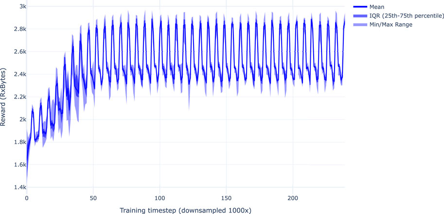
Figure 4. Training convergence of the SAC-RE policy across 10 independent training runs in the periodic traffic scenario. The x-axis represents the training step (averaged over intervals of 1000 steps), and the y-axis shows the total number of received bytes. The observed pronounced spikes result from the injected traffic pattern. The learning process of different instances begins with a higher variance in the reward signal. Over time, the averaged interquartile range tends to shrink, maintaining a consistent appearance at points where the traffic pattern changes.

The training convergence plot indicates that SAC-RE consistently learns an effective policy in the periodic scenario, exhibiting a reward progression over time that aligns with the underlying traffic pattern.

3.1.2 Selection of best model

During the training of all reinforcement learning policies, snapshots of the model weights are periodically saved to allow selection of the best model achieved so far. Figure 5 illustrates the manual selection procedure described in Section 2.4, used to determine which model snapshot to use for inference. As highlighted by the orange dotted line in both plots, the selected training step corresponds to a point where the objective function has plateaued, while the average latency penalty has not yet started to increase. This choice avoids selecting a model that excessively prioritizes the objective function at the cost of violating system constraints.

Figure 5

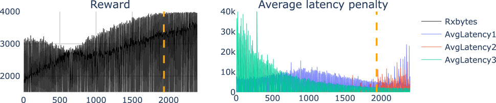
Figure 5. Model selection - This figure shows the objective function (left) and system constraints (right) of the RE policy during the training procedure. The x-axis represents training steps (downsampled by ×100 for visualization). The orange dotted line indicates the manually selected model snapshot used for inference.

3.2 Slicing evaluations with model-free approaches in ns-3

In this section, the inference results of all evaluated policies are presented. The inference times for each policy are shown in Table 2.

Table 2

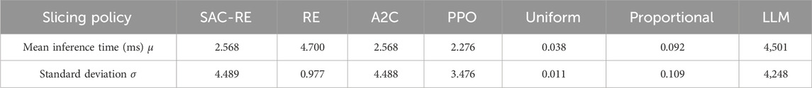
Table 2. Inference time statistics for slicing decision across different policies. Note that response time of the commercial LLM is in the order of seconds, with high variability depending on current service demand.

Figures 6, 7 present the evaluation results of all seven policies under the periodic traffic and random walk traffic scenarios, respectively. In both figures, Column (A) shows the traffic demand per slice, with each slice represented by a distinct color. The x-axis corresponds to the episode step from the RL environment’s perspective. As described in Section 2.4.3, each step represents 0.1 s in the NS3 simulation. Two full episodes (each consisting of 100 steps) are displayed. Column (B) shows the slicing decisions made by the policy at each episode step, visualized as a stacked plot. This represents the proportion of radio resources (ranging from 0 to 1) allocated to each slice over time. Column (C) displays the corresponding reward signal, measured as the total amount of received bytes. Column (D) shows the average constraint penalty metric, which, as defined in Section 2.2, penalizes all packets that were enqueued but not successfully delivered to their destination.

Figure 6

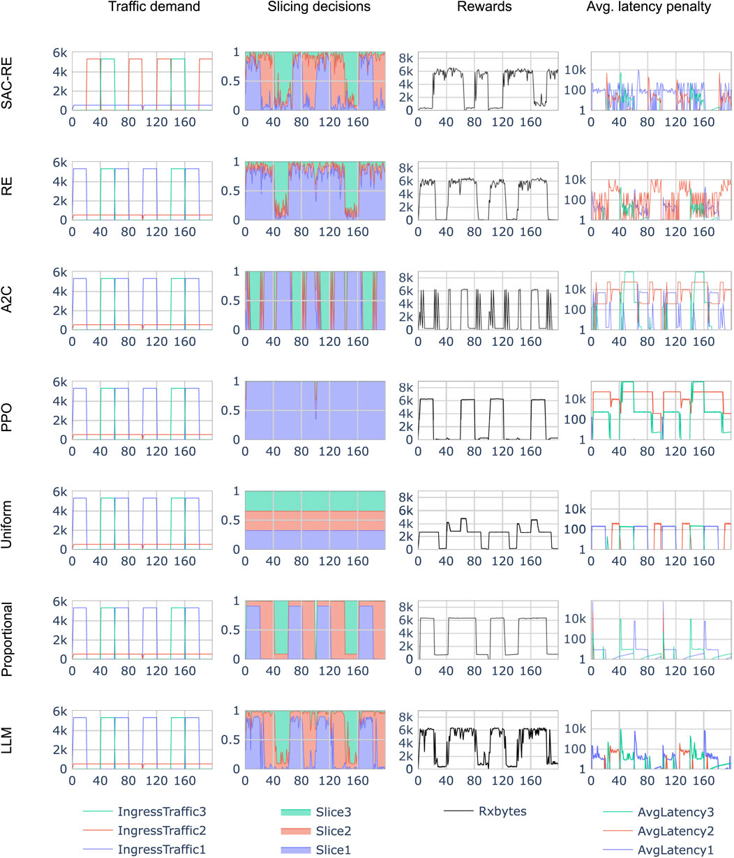
Figure 6. Comparison of different slicing policies (row-wise) in the periodic traffic scenario. Shown are only the first 200 inference time steps of in the x-axis. Columns: (Traffic demand) Input system state, (Slicing decisions) Policy actions, (Rewards) Total received bytes, and (Average latency penalty) RL Constraint.

Figure 7

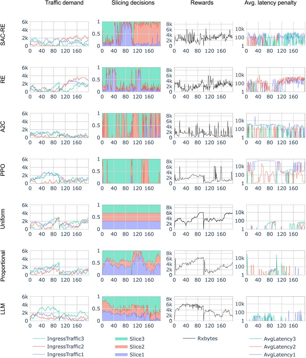
Figure 7. Comparison of different slicing policies (row-wise) in the random walk traffic scenario. Only the first 200 inference time steps are shown on the x-axis. Columns: (Traffic demand) Input system state, (Slicing decisions) Policy actions, (Rewards) Total received bytes, and (Average latency penalty) RL Constraint.

3.2.1 Observations to inference results

When comparing the slicing decisions with the system state in Figure 6, it can be observed that SAC-RE tends to allocate most resources to the slice with the highest current demand. For example, note the high percentage of resources allocated to the low-traffic blue slice during the first 20 steps—reflecting the absence of competing demand. In contrast, RE does not appear to allocate significant resources to the low-throughput slice, even when no other slice is active. This is evident in the limited allocation to the red slice during the 20–40 step interval, despite its being the only active flow.

The other RL approaches, PPO and A2C, failed to effectively adapt to the periodic traffic pattern simulated in ns-3. A2C produced saturated decisions, allocating all resources to a single slice—though not consistently to the one with the highest demand. PPO, on the other hand, consistently assigned all resources to the blue slice. These outcomes suggest that both PPO and A2C may require extensive hyperparameter tuning to perform well in this environment.

The LLM-based policy closely mirrors the proportional heuristic, with a notable bias toward slice 2 — consistent with the prompt used. However, its relatively high inference time, not accounted for in the simulation, limits its practicality in real-time scenarios. In its current form, an unoptimized commercial off-the-shelf LLM may only be suitable for applications with time constraints on the order of seconds. To make LLMs viable for real-world Wi-Fi slicing applications operating on sub-second timescales, inference latency would need to be significantly reduced using existing optimization techniques.

3.3 Policy comparison

To facilitate a clearer comparison of the different policies, Figures 8, 9 summarize the reward and constraint metrics over time as a single average value per traffic scenario.

Figure 8

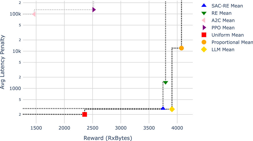
Figure 8. Comparison of slicing policies for the periodic traffic pattern. The lower-right region represents the ideal trade-off between high reward and low constraint penalty. Multiple Pareto fronts are plotted using dotted lines, with the first front representing the set of non-dominated solutions and subsequent fronts indicating decreasing levels of optimality.

Figure 9

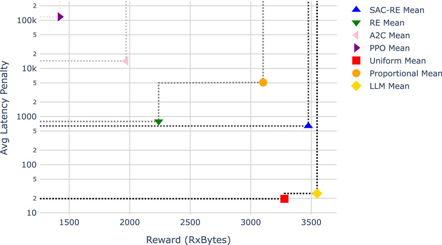
Figure 9. Comparison of slicing policies for the random walk traffic pattern. The lower-right region represents the ideal trade-off between high reward and low constraint penalty. Multiple Pareto fronts are plotted using dotted lines, with the first front representing the set of non-dominated solutions and subsequent fronts indicating decreasing levels of optimality.

The ideal solution is located in the lower-right region of each Figure, representing both high reward and low constraint penalty. Since it is often not possible to simultaneously optimize both objectives in challenging scenarios, a common approach is to visualize the Pareto front to compare the performance of competing solutions. In multi-objective optimization, the Pareto front represents a set of non-dominated solutions—that is, no other solution is strictly better in all objectives. A solution is said to dominate another if it improves at least one objective without worsening any other. However, solutions on the Pareto front cannot be ranked relative to each other, as they reflect trade-offs between competing goals. In Figures 8, 9, multiple Pareto fronts are plotted sequentially to visualize the performance tiers of each policy.

3.3.1 Periodic traffic scenario

Figure 8 shows that the uniform, Proportional, and LLM-based policies lie on the first Pareto front, identifying them as dominating solutions. They are followed by SAC-RE and RE on the second Pareto front, and finally by A2C and PPO. In this scenario, the LLM-based policy is positioned at a favorable trade-off point between reward and constraint satisfaction. Note that the y-axis uses a logarithmic scale, which emphasizes that even small horizontal shifts (i.e., in reward) can correspond to substantial changes in the constraint penalty.

3.3.2 Random walk traffic scenario

In the random walk traffic scenario, shown in Figure 9, the uniform and LLM-based policies again dominate, appearing on the first Pareto front. This time, the SAC-RE policy represents the entire second Pareto front, demonstrating stronger relative performance compared to other RL approaches. The RE and Proportional policies fall to the third front, followed by A2C, and finally PPO. Unlike in the period scenario, the Proportional policy no longer qualifies as a Pareto-optimal solution.

3.4 Inspection of a sample LLM response

In this section, we examine the behavior of the LLM-based policy for a single inference instance to better understand the “reasoning” behind its slicing decision. The sampled system state vector $s$, used as input to the $data$ placeholder in the llm_policy prompt template, is given by:

$s=\left[0.0,0.0,0.0,0.0,0.0,0.0,5357.0,535.0,6.0,5357.0,536.0,5.0,5357.0,536.0,6.0,5357.0,535.0,5.0\right]$

The corresponding full response generated by the LLM for this prompt is shown in Box 2:

Box 2 LLM response.
To determine the optimal allocation of resources among the three network slices, let’s analyze the given input data, which includes the current traffic demand and the historical traffic demand for the last five intervals.

Input: [0.0, 0.0, 0.0, 0.0, 0.0, 0.0, 5357.0, 535.0, 6.0, 5357.0, 536.0, 5.0, 5357.0, 536.0, 6.0, 5357.0, 535.0, 5.0].

1. The current demand vector is [5357.0, 535.0, 5.0]. 2. The historical demands show a consistent pattern where slice #1 has the highest demand, followed by slice #2, and slice #3 has minimal demand.

Given the decision objective, we need to prioritize slice #2 to ensure it can always transmit packets, and we should allocate resources based on demand while maintaining fairness and avoiding excessive fluctuations.

Considering the historical trend and current demand:

- Slice #1 (demand: 5357.0) has the highest demand.

- Slice #2 (demand: 535.0) must be protected for time-critical packets.

- Slice #3 (demand: 5.0) has the lowest demand.

We will allocate bandwidth proportionally to the demand, ensuring slice #2 gets sufficient resources, and then distribute the remaining bandwidth between slices #1 and #3.

Let’s calculate the allocation:

- Total demand: 5357.0 + 535.0 + 5.0 = 5897.0.

- Allocate a base of 0.3 to slice #2 (time-critical protection).

- Remaining proportion: 1.0–0.3 = 0.7.

Allocation based on demand:

- Slice #1: (5357.0/5897.0) * 0.7 $\approx$ 0.636.

- Slice #2: 0.3 (protected).

- Slice #3: (5.0/5897.0) * 0.7 $\approx$ 0.001.

Final allocation:

- Slice #1: 0.636.

- Slice #2: 0.3.

- Slice #3: 0.064 (adjusting for the remaining sum to 1).

The final allocation vector is: [0.636, 0.3, 0.064].

From this response, the parser extracted the following vector as the slicing decision:

$a=\left[0.6360,0.3000,0.0640\right]$

The prompt template used enabled the LLM to “reason” step by step through the task. This approach helps reduce hallucinations, as prompting for an immediate direct answer may cause the LLM to rely too heavily on memorized patterns from its training data, rather than drawing on higher-level reasoning processes—which are likely more robust and broadly represented in its training corpus. As observed in this instance, the heuristic followed by the LLM begins by allocating a fixed base of 30% to slice 2 to ensure a minimum level of resources. The remaining budget is then distributed proportionally across the other slices, based on patterns inferred from the historical system state. However, the LLM proposed an erroneous split of the 70% remainder, as it normalized against the total demand (5897) instead of using only the sum of the demand for slice 1 and slice 3. The model ultimately corrected the flawed formula by allocating more resources to slice 3 to ensure that the sum adds up to 1.

4 Discussions

4.1 Best slicing policies

Our results in Figures 8, 9 show that, when averaging across an entire inference scenario—in terms of total throughput versus average latency penalty—the uniform, proportional, and the LLM-based policies dominate the others in the periodic traffic pattern scenario, with the LLM policy effectively balancing both the reward and latency constraint. In the random walk scenario, the proportional policy is no longer part of the first Pareto front, being surpassed by the SAC-RE RL policy as well. This indicates that the RL based policies were not able to predict the traffic patterns as effectively. Among them, the state-augmented version of REINFORCE SAC-RE performed best. This can be attributed to its ability to model multiple modes of operation and achieve better performance, even without extensive hyper-parameter tuning, thanks to the use of the state augmentation.

The LLM policy on the other hand—which was not re-trained nor fine-tuned on any data—appears at the first Pareto front in both scenarios, providing a higher value of the objective function at some cost to the latency constraint. Unlike the uniform slicing approach, the LLM policy’s behavior can be adjusted via prompt alone. Thus, the LLM policy thus provides a flexible and easy-to-setup slicing approach, as it can leverage the knowledge encoded in the foundational LLM to decide which action to take without requiring an extensive training. The main cost of this approach lies in the expensive inference calls, both in terms of compute resources and inference latency. However, recent progress in knowledge distillation (Acharya et al., 2024) and model pruning of LLMs into smaller models (Ma et al., 2023) has made promising steps towards mitigating high latency in LLMs. In terms of inference latency, the main limiting factor arises from the long prompt and model response that must be processed sequentially. The good news is that this too can be mitigated, through fast fine-tuning techniques (Han et al., 2024) which allow a foundational LLM to be modified such that smaller prompts yield the same output.

In terms of scalability regarding the number of slices, as the number of slices increases, the effectiveness of learning-based policies would be affected because both the state space and the action space increase accordingly. This leads to longer training periods and convergence issues. The maximum number of slices would be limited by the available Resource Units (RUs) in the deployed system. In Wi-Fi 6 (802.11ax), the theoretical maximum number of RUs available in a 160 MHz channel is 996. However, typical deployments often use smaller channel bandwidths due to regulatory constraints and spectrum availability. For a 20 MHz channel, there are up to 9 RUs available. On the technical implementation side, if the User Priority (UP) field of Wi-Fi is used to map packets to slices, the number of slices would be limited to 8. For the LLM policy, as the Wi-Fi network scales in complexity, e.g., with more slices, the prompt fed to the LLM would have an impact on the latency of the response, as the ”reasoning” of the LLM would describe more computations or consequences for each of the managed resources. The exact scaling factor will depend on the conditioning prompt.

4.2 Impact of state augmentation in REINFORCE

In addition, it is worth noting that the results show a more significant improvement from integrating the state-augmented approach into the REINFORCE algorithm (SAC-RE) in the more challenging scenario. As shown in Figure 9, SAC-RE appears on the second Pareto front in the random walk scenario, dominating the vanilla RE approach without state-augmentation. In contrast, in the periodic scenario (Figure 8), RE is co-located with SAC-RE on the second Pareto front, albeit with a significant trade-off in latency.

4.3 Conclusion

In conclusion, we confirmed the benefit of adding state augmentation to reinforcement learning solutions for systems exhibiting multi-modality, as the implemented SAC-RE solution outperformed the other RL approaches under a similarly low-cost, manually tuned hyper-parameter settings. The most promising result is the performance of the LLM-based policy, which required no training or optimization and, out-of-the-box, provided a dominating solution that can be further guided through prompt design. As LLM optimization techniques continue to evolve, it should become increasingly feasible to deploy LLM-based policies in low-cost scenarios as well.

Data availability statement

Publicly available source code was analyzed in this study. This data can be found here: https://gitlab.netcom.it.uc3m.es/predict-6g/AI-based_Wi-Fi_Slicing.

Author contributions

RR: Conceptualization, Investigation, Methodology, Visualization, Writing – original draft, Writing – review and editing. DC: Funding acquisition, Supervision, Writing – review and editing.

Funding

The author(s) declare that financial support was received for the research and/or publication of this article. This work has been partially funded by the European Commission Horizon Europe SNS JU PREDICT-6G (GA 101095890) Project.

Conflict of interest

Authors RR and DC were employed by Intel Corporation.

Generative AI statement

The author(s) declare that Generative AI was used in the creation of this manuscript. Generative AI was used to correct grammar of human writing.

Publisher’s note

All claims expressed in this article are solely those of the authors and do not necessarily represent those of their affiliated organizations, or those of the publisher, the editors and the reviewers. Any product that may be evaluated in this article, or claim that may be made by its manufacturer, is not guaranteed or endorsed by the publisher.

References

Acharya, K., Velasquez, A., and Song, H. H. (2024). A survey on symbolic knowledge distillation of large language models. IEEE Trans. Artif. Intell. 5, 5928–5948. doi:10.1109/TAI.2024.3428519

CrossRef Full Text | Google Scholar

Brockman, G., Cheung, V., Pettersson, L., Schneider, J., Schulman, J., Tang, J., et al. (2016). Openai gym. arXiv preprint arXiv:1606.01540

Google Scholar

Calvo-Fullana, M., Paternain, S., Chamon, L. F. O., and Ribeiro, A. (2023). State augmented constrained reinforcement learning: overcoming the limitations of learning with rewards.

Google Scholar

Candell, R., Montgomery, K., Hany, M. K., Sudhakaran, S., Albrecht, J., and Cavalcanti, D. (2022). “Operational impacts of IEEE 802.1qbv scheduling on a collaborative robotic scenario,” in Iecon 2022 - 48th annual Conference of the IEEE industrial electronics society (Brussels, Belgium: IEEE), 1–7. doi:10.1109/IECON49645.2022.9968494

CrossRef Full Text | Google Scholar

Han, Z., Gao, C., Liu, J., Zhang, J., and Zhang, S. Q. (2024). Parameter-efficient fine-tuning for large models: a comprehensive survey. Corr. abs/2403, 14608. doi:10.48550/ARXIV.2403.14608

CrossRef Full Text | Google Scholar

Henderson, T. R., Lacage, M., Riley, G. F., Dowell, C., and Kopena, J. (2008). Network simulations with the ns-3 simulator. SIGCOMM Demonstr. 14, 527.

Google Scholar

Kingma, D. P., and Ba, J. (2015). “Adam: a method for stochastic optimization,” in 3rd international conference on learning representations, ICLR 2015. Editors Y. Bengio, and Y. LeCun (San Diego, CA: Conference Track Proceedings).

Google Scholar

Liu, Q., Choi, N., and Han, T. (2021). “Onslicing: online end-to-end network slicing with reinforcement learning,” in Proceedings of the 17th international conference on emerging networking EXperiments and technologies (New York, NY, USA: Association for Computing Machinery), 21, 141–153. doi:10.1145/3485983.3494850

CrossRef Full Text | Google Scholar

Liu, Y., Ding, J., and Liu, X. (2020). “A constrained reinforcement learning based approach for network slicing,” in 2020 IEEE 28th international conference on network protocols (ICNP), 1–6. doi:10.1109/ICNP49622.2020.9259378

CrossRef Full Text | Google Scholar

Ma, X., Fang, G., and Wang, X. (2023). “Llm-pruner: on the structural pruning of large language models,” in Advances in neural information processing systems 36: annual conference on neural information processing systems 2023. Editors A. Oh, T. Naumann, A. Globerson, K. Saenko, M. Hardt, and S. Levine (New Orleans, LA: NeurIPS).

Google Scholar

Mnih, V., Badia, A. P., Mirza, M., Graves, A., Lillicrap, T. P., Harley, T., et al. (2016). “Asynchronous methods for deep reinforcement learning,” in Proceedings of the 33nd international conference on machine learning, ICML 2016. Editors M. Balcan, and K. Q. Weinberger (New York City, NY: JMLR.org), 48, 1928–1937.

Google Scholar

NaderiAlizadeh, N., Eisen, M., and Ribeiro, A. (2022). State-augmented learnable algorithms for resource management in wireless networks. IEEE Trans. Signal Process. 70, 5898–5912. doi:10.1109/TSP.2022.3229948

CrossRef Full Text | Google Scholar

Peng, S., Hu, X., Zhang, R., Guo, J., Yi, Q., Chen, R., et al. (2023). Conceptual reinforcement learning for language-conditioned tasks. Proc. AAAI Conf. Artif. Intell. 37, 9426–9434. doi:10.1609/aaai.v37i8.26129

CrossRef Full Text | Google Scholar

Rosales, R. (2025). Python implementation of SAC-RE algorithm. Available online at: https://gitlab.netcom.it.uc3m.es/predict-6g/AI-based_Wi-Fi_Slicing (Accessed March 14, 2025).

Google Scholar

Schulman, J., Wolski, F., Dhariwal, P., Radford, A., and Klimov, O. (2017). Proximal policy optimization algorithms. Corr. abs/1707, 06347.

Google Scholar

Stable-Baselines3 (2025a). Proximal policy optimization algorithm. Available online at: https://stable-baselines3.readthedocs.io/en/master/modules/ppo.html (Accessed March 14, 2025).

Google Scholar

Stable-Baselines3 (2025b). Synchronous, deterministic variant of asynchronous advantage actor critic (A3C). Available online at: https://stable-baselines3.readthedocs.io/en/master/modules/a2c.html (Accessed March 14, 2025).

Google Scholar

Sutton, R. S., and Barto, A. G. (1998). Reinforcement learning: an introduction, 1. MIT press Cambridge.

Google Scholar

Uslu, Y. B., Doostnejad, R., Ribeiro, A., and NaderiAlizadeh, N. (2024). “Learning to slice wi-fi networks: a state-augmented primal-dual approach,” in Globecom 2024 - 2024 IEEE global communications conference, 4521–4527. doi:10.1109/GLOBECOM52923.2024.10901174

CrossRef Full Text | Google Scholar

Williams, R. J. (1992). Simple statistical gradient-following algorithms for connectionist reinforcement learning. Mach. Learn. 8, 229–256. doi:10.1007/BF00992696

CrossRef Full Text | Google Scholar

Yang, K., Yeh, S.-P., Zhang, M., Sydir, J., Yang, J., and Shen, C. (2024). “Advancing ran slicing with offline reinforcement learning,” in 2024 IEEE international symposium on dynamic spectrum access networks (DySPAN), 331–338. doi:10.1109/DySPAN60163.2024.10632750

CrossRef Full Text | Google Scholar

Yin, H., Liu, P., Liu, K., Cao, L., Zhang, L., Gao, Y., et al. (2020). “ns3-ai: fostering artificial intelligence algorithms for networking research,” in Proceedings of the 2020 workshop on ns-3, WNS3 2020. Editors R. Rouil, S. Avallone, M. Coudron, and E. Gamess (Gaithersburg, MD: ACM), 57–64. doi:10.1145/3389400.3389404

CrossRef Full Text | Google Scholar

Zangooei, M., Saha, N., Golkarifard, M., and Boutaba, R. (2023). Reinforcement learning for radio resource management in ran slicing: a survey. IEEE Commun. Mag. 61, 118–124. doi:10.1109/MCOM.004.2200532

CrossRef Full Text | Google Scholar

Zhang, S. (2019). An overview of network slicing for 5g. IEEE Wirel. Commun. 26, 111–117. doi:10.1109/mwc.2019.1800234

CrossRef Full Text | Google Scholar

Zhou, L., and Small, K. (2021). Inverse reinforcement learning with natural language goals. Proc. AAAI Conf. Artif. Intell. 35, 11116–11124. doi:10.1609/aaai.v35i12.17326

CrossRef Full Text | Google Scholar