Electric vehicle scheduling strategy based on dynamic adjustment mechanism of time-of-use price

As the grid-connected capacity of distributed photovoltaic (PV), energy storage, electric vehicle (EV), and other devices gradually increases, new source-load equipment becomes an important demand response (DR) resource in the distribution network (DN). To fully utilize the DR's capability for EVs and other devices and reduce the system operating costs and line network loss, this article presents a DR scheduling strategy for EVs based on a time-of-use (TOU) price dynamic adjustment mechanism. First, a fuzzy C-mean (FCM) clustering algorithm is used to calculate the typical operating curves of PV and electrical load and their optimal number of classifications. The deterministic scenarios express the PV's output characteristics and the users' electricity consumption characteristics. Second, a dynamic adjustment mechanism of TOU price is proposed based on the load operation curve of the DN, and the interactive price-incentive signal for DR within the DN is formulated. Finally, a DR scheduling strategy for EVs in the DN that considers the economic cost of system operation and line network loss is proposed. CPLEX in MATLAB is employed to simulate the cases. After applying the TOU price dynamic adjustment mechanism proposed, the peak total load and peak–valley load difference decreased by 6.9% and 33.8%, respectively, compared to implementing fixed electricity prices. At the same time, the operating revenue of the distribution network increased by 13.2%, and the line network loss decreased by 12.9%. The analysis results demonstrate that the proposed EV DR scheduling strategy can realize the price guidance and orderly scheduling of EVs and reduce the operation cost and line network loss in the DN.

1 Introduction

With the transformation of the global energy structure and the diversification of power generation and utilization, the distribution network (DN) is gradually transforming into a new distribution system containing a high proportion of distributed photovoltaics (PVs), energy storage devices, and electric vehicles (EVs; Xu et al., 2023). Among these factors, the variability of PV output and load fluctuation pose a challenge to the stable operation of the DN (Alamolhoda et al., 2024). To solve these problems, experts are gradually tapping the interactive potential of various demand-response (DR) resources to participate in grid regulation and formulating more effective DN operation modes and time-of-use (TOU) price mechanisms (Sun et al., 2024).

An important means for guiding subjects in the DN to participate in the DR (Choi and Murali, 2022), research related to the TOU price policy for DNs has attracted extensive attention. To achieve the minimization of comprehensive operating costs, a peak–valley TOU price optimization model can be established by considering the power generation–side, grid-side, and user-side revenue (Ahsan et al., 2023). A TOU price optimization method for PV admittance capacity improvement in DNs can also be proposed from the user side. The imperialist competitive algorithm is used to solve the TOU price (Shabbir et al., 2024). The improved price elasticity matrix model based on elasticity effect weights can also be used to analyze users' responses to TOU price, and combined with genetic algorithms, the decision-making model of TOU price can be solved (Xue et al., 2023). Most of the mentioned studies focus on establishing various TOU price models from different stakeholders' perspectives and using different solution algorithms to realize the accurate calculation of TOU price; they do not conduct in-depth research on the periods' division of TOU price and the dynamic adjustment of TOU price.

In recent years, in research on DN optimization and operation, scene generation and vehicle-network interaction have gradually become hot issues. The random scenes of wind speed, light intensity, electrical load, and thermal load can be simulated using the Monte Carlo method and optimized using the particle swarm algorithm for scene selection (Fu et al., 2020). Some literature proposes combining a multidimensional representative scene generation algorithm based on load clustering with the K-means clustering method to extract representative scenes of PV and wind power (Gao et al., 2023). Intelligent algorithms based on parameter-sharing frameworks can quantify EVs' ability to participate in DR and voltage regulation services in DNs for power coordination control (Wang et al., 2023). Using an improved robust model predictive control strategy in microgrids can effectively utilize EVs for frequency control, improving the stability and robustness of the DN (Rao et al., 2021). By combining the peak-shaving requirements of the system, a vehicle–grid interaction incentive pricing mechanism can be developed to smooth the system's electrical load curve and improve the DN's operational economy (Yin et al., 2023). These studies do not accurately calibrate the reasonableness of the clustering results and have not taken into account the line network loss and operating revenue of the DN for multi-objective scheduling.

As an important means of guiding various entities in the DN to participate in DR (Yang et al., 2013), research on TOU price in the DN has attracted widespread attention from scholars worldwide. At present, research methods on electricity pricing mechanisms mainly focus on reducing the operating costs of DNs, improving PV consumption rates, and incentivizing users to participate in DR. Each method's characteristics are shown in Table 1. Some literature considers the interests of the power generation side, grid side, and demand side to establish a TOU electricity price optimization model, achieving the minimization of comprehensive operating costs (Imani et al., 2019; Pandey et al., 2022; Zhang et al., 2025). Some TOU price optimization methods start from the user side, design objective functions for the PV acceptance capacity of the DN, and use different optimization algorithms to solve the TOU price (Yang et al., 2020; Magdy et al., 2021). By calculating an improved price elasticity matrix model based on elastic effect weights, EVs' response to TOU pricing can be analyzed, and a decision-making model for the TOU price can be solved using genetic algorithms (Ma et al., 2022; Kaur and Singh, 2023; Song et al., 2021; Zhou et al., 2020). The mentioned research mainly focuses on establishing various TOU price models from different stakeholders and using different solving algorithms to achieve the accurate calculation of TOU pricing without in-depth research on the division of the TOU price periods and the dynamic adjustment of the TOU price.

Table 1

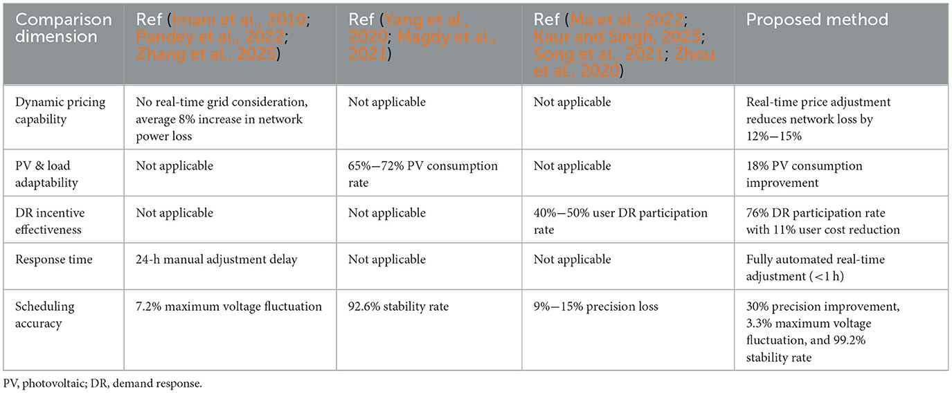
Table 1. The technical comparison between proposed controller and existing controllers.

To address the aforementioned problems, this article presents a DR scheduling strategy utilizing the TOU price dynamic adjustment mechanism for EVs. First, methods for extracting typical PV output and regional load scenarios, as well as methods for generating EV charging loads, are presented. Second, a hierarchical clustering algorithm is used to classify the comprehensive load into periods. Then, a load electricity price elasticity matrix is established to quantify the role of TOU pricing in guiding loads, combined with the implementation of DR to establish a more efficient guiding TOU price mechanism. Finally, a comprehensive objective function is constructed by considering the operating revenue and line network loss and combining the constraints of each subject in the DN to schedule their operation status. An optimization scheduling model is constructed with the following decision variables: electricity price, consumption of PV output, charging and discharging power of energy storage, charging and discharging quantity of EVs, and the number of load reductions that can be made in each time period. This model belongs to the mixed-integer programming problem, so the Cplex solver in the Yalmip platform is called on to solve the problem to achieve the goal of improving the operating income of the DN and reducing the line network loss.

The remainder of the article is organized as follows: Section 2 introduces the generation methods of PV, regional load, and EV charging curves. Section 3 proposes a dynamic adjustment mechanism for TOU electricity prices. Section 4 constructed a DR scheduling model for the DN. Simulation and analysis are given in Section 5. Section 6 concludes the article with a discussion.

2 Typical PV and electrical load curves

The difficulty of optimal scheduling of DNs is the uncertainty of PV output and electricity consumption characteristics. Although the power curves exhibit a certain regularity overall, differences also exist between them. This article adopts the fuzzy C-means clustering algorithm (FCM) to cluster the PV and regional load curves in the DN to generate typical curves. This method not only comprehensively considers various situations of electricity consumption and PV output but also reduces the computational complexity. Meanwhile, based on EV travel data, the Monte Carlo method is used to generate the EV charging load curve.

2.1 FCM

FCM is a clustering method that utilizes the objective function, where the degree to which each sample data point belongs to a certain cluster is determined by membership degree, and it has the characteristics of fuzzy soft clustering (Yang et al., 2024). This algorithm has the characteristics of simple design and easy implementation. It can also use non-linear theory to solve optimization algorithms with a wide range of applications. The FCM clustering method flowchart is shown in Figure 1.

Figure 1

Figure 1. The flowchart of the fuzzy C-means clustering method (FCM). PV, photovoltaic.

The FCM clustering method first preprocesses historical PV and load data and selects the appropriate clustering indicators. Then, the clustering indicators and scene clustering centers are iteratively calculated using the Lagrange multiplier method, and the likelihood of each sample belonging to each clustering center is calculated to obtain the PV and load curves' clustering results.

The objective function of FCM includes two indexes: the cluster center and the membership matrix. After selecting the clustering indicators, the number of clusters and the optimal clustering curves when the objective function takes the minimum value are iteratively solved.

2.1.1 Clustering process

Supposing a data set matrix X is

$\begin{array}{ll}X=\left\{x_1,\cdots ,x_t,\cdots ,x_T\right\}& (1)\end{array}$

where T is the total number of samples contained in the PV or load sample data set, T = 24, and x_t is the vector of feature aggregation metrics for the tth sample.

The objective function of FCM is defined as follows:

$\begin{array}{ll}min{J}_{FCM}(\lambda ,\eta )={\displaystyle \sum _{l=1}^m}{\displaystyle \sum _{t=1}^T}{u}_{lt}^m{D}_{x_{l,t}}^2& (2)\end{array}$

where λ is the scene clustering affiliation matrix with matrix size m × T; m is any given number of initial clusters, η is the clustering center matrix with matrix size m × z; z is the number of clustering indicators for each PV or load sample; l indicates category, lε[1,m]; u_lt is the probability that the tth sample belongs to category l; ${\sum }_{l=1}^m{u}_{lt}=1,u_{lt}\in \left[0,1\right]\forall l,t$. D_{xl, t} = |x_t−v_l|, D_{xl, t}is the Euclidean distance between the sample data, which is used to characterize the similarity between the vectors; AM is the degree of fuzziness; and v_l is the lth clustering center.

The optimal sample clustering likelihood indicator u_lt and scene clustering center v_l in the objective function can be computed iteratively by the Lagrange multiplier method (Chaouch, 2013; Rajabi et al., 2020).

2.1.2 PV clustering index

PV output is random and fluctuates due to weather, season, holidays, and other conditions. To extract the PV output curve's fluctuation characteristics and enhance the accuracy of clustering, selecting appropriate clustering indicators is necessary. Therefore, the daily average output, the daily output volatility, and the daily output distribution skewness are selected as the PV output characteristic clustering indexes.

Considering the daily output characteristics, the average PV output during the day is calculated:

$\begin{array}{ll}{P}_{PV}^m={\displaystyle \sum _{t=1}^T}\frac{P_{PV}^t}{T}& (3)\end{array}$

where $P_{PV}^m$ is the average daily power generated by PV and $P_{PV}^t$ is power produced by PV at time t.

The daily output volatility is utilized to describe the level of volatility of the PV curve. The smaller the value of this characteristic, the smaller the fluctuation of the day's PV output curve:

$\begin{array}{ll}{\gamma }_{PV}=\sqrt{\frac{1}{T-1}{\displaystyle \sum _{t=1}^T}{(P_{PV}^t-P_{PV}^m)}^2}& (4)\end{array}$

where γ_PV is the volatility of daily PV output.

The skewness of the daily output distribution can be used to describe the degree of daily skewness of the PV output. When the skewness value is between [−0.5, 0.5], the force distribution is relatively symmetrical. When the skewness value is between [0.5, +∞), the force distribution is positively skewed and concentrated on the right side of the mean. When the skewness value lies between [–∞, −0.5], the force distribution is negatively skewed, and the force is concentrated on the left side of the mean:

$\begin{array}{ll}S{K}_{PV}=\frac{T}{(T-1)(T-2)}{\displaystyle \sum _{t=1}^T}{(\frac{P_{PV}^t-P_{PV}^m}{{\gamma }_{PV}})}^3& (5)\end{array}$

where SK_PV is the skewness of the daily PV output distribution.

2.1.3 Regional load clustering index

Selecting the appropriate load clustering indexes can more comprehensively reflect the curve characteristics and improve the speed of solving the scheduling model. The load rate, the maximum utilization hour rate, and the daily peak-to-valley difference rate are selected from an all-day perspective, the peak load rate from a peak-period perspective, the flat-period load rate from a flat-period perspective, and the valley load rate from valley-period perspective as the load clustering indexes (Satre-Meloy et al., 2020). It comprehensively combines the electricity consumption characteristics of loads for clustering processing.

2.2 Modeling of charging load for EVs

A large number of EVs are in the DN, and their disorderly charging and discharging characteristics increase the peak load, which has a significant impact on the operation of the DN. As a result, establishing a charging load model for EVs and scheduling them accordingly are necessary. The disorder in EV charging is reflected in the uncertainty and unpredictability of the charging start time and charging time. According to U.S. Department of Transportation statistical data on EV travel in the United States (Ren et al., 2024), a probability model for daily EV travel is calculated.

The end time of the last trip of an EV in a single day is equivalent to the start time of EV charging, following a normal distribution. The normal distribution function is used to describe the starting time of EV charging:

$\begin{array}{ll}f(x_c)=\frac{1}{{\sigma }_c\sqrt{2\pi }}exp[-\frac{{(x_c-{\mu }_c)}^2}{2{\sigma }_c^2}]& (6)\end{array}$

where x_c is a random variable representing the starting time of EV charging.

The daily mileage of EVs has a certain regularity. This article employs a logarithmic normal distribution function to describe the daily mileage of EVs:

$\begin{array}{ll}f(x_s)=\frac{1}{x_s}\frac{1}{{\sigma }_s\sqrt{2\pi }}exp[-\frac{{(ln{x}_s-{\mu }_s)}^2}{2{\sigma }_s^2}]& (7)\end{array}$

here x_s is a random variable representing the daily mileage of EV.

The charging time of an EV is defined as

$\begin{array}{ll}{T}_{EV}=x_s{X}_d^{100}/100P_{cd}{\eta }_c& (8)\end{array}$

where $X_d^{100}$ is the power consumption of an EV for driving 100 kilometers, P_cd is the charging power of an EV, and η_c is the charging efficiency of an EV.

The EV's charging load curve is obtained using the Monte Carlo method (Shan et al., 2025).

3 TOU price model

Adopting a TOU price model can change users' electricity consumption habits and reduce DN costs (Venizelou et al., 2018). With the increase in the number of EVs, combining their charging demand with regional electricity demand as a comprehensive load for co-participation scheduling can not only avoid power shortages during peak hours but also increase the DN's stability (Nicolson et al., 2018). It is evident that completing the TOU price mechanism in which EV loads and regional loads co-participate in DR is crucial.

First, a hierarchical clustering method is used to divide the comprehensive load at each moment into periods. On this basis, the relationship between time period load and TOU price is studied, and the load electricity price elasticity coefficient matrix is derived. Furthermore, a TOU price model is established to solve the TOU price for each period.

3.1 TOU price period division method

Due to the increase in the types and quantities of loads, such as EVs in the power system, midday loads regularly have low troughs. The charging time of EVs overlaps with the evening peak time, resulting in an increase in the peak valley difference for the load curve (Li et al., 2023), making the load curve characteristics more complex.

Using the hierarchical clustering method to classify periods can effectively aggregate electricity consumption periods with similar loads. The hierarchical clustering method can effectively aggregate the periods with similar loads and cluster the samples of comprehensive load periods without setting the number of periods in advance.

In the hierarchical clustering process, based on the input comprehensive load at each moment of the P_SL, the degree of similarity between loads of any two time periods can be quantified as the Euclidean distance D_{PSL, i, j} between the comprehensive load samples:

$\begin{array}{ll}{D}_{P_{SL,i,j}}=|P_{SL,i}-P_{SL,j}|,i,j=1,2,\cdots ,24& (9)\end{array}$

As P_{SL, i} and P_{SL, j} get closer, the value of D_{PSL, i, j} gets smaller. Conversely, as P_{SL, i} and P_{SL, j} get farther apart, the value of D_{PSL, i, j} gets larger. From this, a 24 × 24 distance matrix D_PSL between load powers at each moment can be defined:

$\begin{array}{ll}{D}_{P_{SL}}=\left[\begin{array}{cccc}0& D_{P_{SL,1,2}}& \cdots & D_{P_{SL,1,24}}\\ D_{P_{SL,2,1}}& 0& \cdots & D_{P_{SL,2,24}}\\ \cdots & \cdots & \ddots & \cdots \\ D_{P_{SL,24,1}}& D_{P_{SL,24,2}}& \cdots & 0\end{array}\right]& (10)\end{array}$

At first, each period load in the matrix is considered to be one category. Then, based on D_PSL, the two time periods corresponding to the minimum non-diagonal elements are merged into a new period. The square of the inter-category distance between the new classification period and other periods can be defined:

$\begin{array}{ll}{D}_{com,re}^2=\frac{n_{in1}}{n_{com}}{D}_{in1,re}^2+\frac{n_{in2}}{n_{com}}{D}_{in2,re}^2& (11)\end{array}$

where D_{in1, re} and D_{in2, re} are the distances between the loadings of the two time periods involved in the merger and the other periods, n_com is the number of periods in the merged new period, and n_in1 and n_in2 are the number of periods in the two categories participating in the merger, respectively.

After completing the kth merge, obtain n-k periods and renumber them as $T_1^{(k+1)}$, $T_2^{(k+1)}$,... $T_{n-k}^{(k+1)}$. These steps are repeated until the final clustering of periods is completed.

3.2 Guiding effect of electricity price on load

Some research has been conducted on quantifying the role of TOU price in directing load. The relationship curve between the electricity supply and the electricity demand is given in the literature (Zhu et al., 2018), as shown in Figure 2. The electricity supply curve illustrates the relationship between the electricity price and the amount of electricity supplied. The electricity demand curve illustrates the relationship between the electricity price and the amount of electrical load. The intersection point represents the equilibrium between the supply and demand of electricity, which is the actual operating point of the power system.

Figure 2

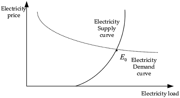
Figure 2. Relationship curves between electricity supply and electricity demand.

3.2.1 Relationship between load and electricity price in the same period

The electricity demand curve in Figure 2 reflects the relationship between the change in electricity price in the current period and the change in electrical load in the same period. It is considered that the electricity price and electrical load approximately satisfy the linear relationship near the market equilibrium point (point E₀ in Figure 2) in each period. The relationship can be defined as

$\begin{array}{ll}{P}_j=-k_j{c}_j+b_j& (12)\end{array}$

where k_j and b_j are the parameters of the linear function for period j, jε[1, J]; P_j is the electricity load in period j; and c_j is the electricity price in period j.

3.2.2 Relationship between load and electricity price in the different periods

To quantify the impact of electricity price changes on electrical load, the concept of price elasticity, which is commonly used in economics, is introduced. Price elasticity measures the extent to which market demand changes in response to price fluctuations. It is expressed as the ratio of the change in load to the change in price in TOU price, which can be expressed using Equation 13:

$\begin{array}{ll}\epsilon =\frac{\Delta P/P}{\Delta c/c}& (13)\end{array}$

where ε is the price elasticity coefficient, P is the amount of comprehensive load, c is the electricity price, ΔP is the change in electrical load, and Δc is the change in the electricity price.

Because changes in electricity price in a given period may affect electrical loads in more than one time period, categorizing the elasticity coefficients as self-elasticity coefficients and cross-elasticity coefficients is necessary (Yang et al., 2023).

3.2.3 Self-elasticity coefficient

The self-elasticity coefficient reflects the effect of electricity price changes on the electrical load during the same period. It is defined using Equation 14:

$\begin{array}{ll}{\epsilon }_{jj}=\frac{\Delta P_j/P_j}{\Delta c_j/c_j}& (14)\end{array}$

where ε_jj is the self-elasticity coefficient in period j, P_j is the original comprehensive load in period j, ΔP_j is the change in comprehensive load after electricity price adjustment during period j, c_j is the original electricity price in period j, and Δc_j is the electricity price change in period j.

According to Equations 12, 14, the self-elasticity coefficients for each period can be obtained using Equation 15:

$\begin{array}{ll}{\epsilon }_{jj}=\frac{-k_j{P}_j}{-k_j{P}_j+b_j}& (15)\end{array}$

3.2.4 Cross-elasticity coefficient

The cross-elasticity coefficient reflects the effect of electricity price changes in other periods on the electrical load in a given period. Taking period 1 and period j as an example, it can be defined using Equation 16:

$\begin{array}{ll}{\epsilon }_{1j}=\frac{\Delta P_1/P_1}{\Delta c_j/c_j}& (16)\end{array}$

where ε_1j is the cross-elasticity coefficient between period 1 and period j, P₁ is the original comprehensive load during period 1, and ΔP₁ is the change in comprehensive load after electricity price adjustment in period 1.

Because load stability constraints are present, the daily comprehensive load can be considered to be a fixed value:

$\begin{array}{ll}{P}_1+\cdots P_j\cdots +P_J=P_L& (17)\end{array}$

Substituting Equation 12 into Equation 17, the equation is simplified:

$\begin{array}{ll}{P}_1-\cdots -k_j{c}_j+b_j-\cdots -k_J{c}_J+b_J=P_L& (18)\end{array}$

Deriving from c_j both sides of Equation 18,

$\begin{array}{ll}\frac{\partial P_1}{\partial c_j}=k_j& (19)\end{array}$

Combining Equations 16, 18, the cross-elasticity coefficient can be obtained:

$\begin{array}{ll}{\epsilon }_{1j}=\frac{c_j}{P_1}·\frac{\partial P_1}{\partial c_j}=\frac{k_j{c}_j}{-k_1{P}_1+b_1}& (20)\end{array}$

The cross-elasticity coefficients for the other periods can be obtained in the same way.

3.2.5 Relationship between electricity load and electricity price changes

According to Equation 13, the comprehensive load change ΔP after electricity price adjustment Δc is obtained using Equation 21:

$\begin{array}{ll}\Delta P=P(\Delta c/c)\epsilon & (21)\end{array}$

The load electricity price elasticity matrix S in 1 day is shown in Equation 22:

$\begin{array}{ll}S=\left[\begin{array}{cccc}{\epsilon }_{11}& {\epsilon }_{12}& \cdots & {\epsilon }_{1N}\\ {\epsilon }_{21}& {\epsilon }_{22}& \cdots & {\epsilon }_{2N}\\ ⋮& ⋮& \ddots & ⋮\\ {\epsilon }_{N1}& {\epsilon }_{N2}& \cdots & {\epsilon }_{NN}\end{array}\right]& (22)\end{array}$

where N = 24. The elements in the diagonal are the self-elasticity coefficients at each moment. The off-diagonal elements are the cross-elasticity coefficients between each moment and the other moments.

In summary, combining Equations 21, 22, the comprehensive load P′ for J periods after electricity price adjustment can be defined using Equation 23:

$\begin{array}{ll}{P}^{\prime }=\left[\begin{array}{ccc}{P}_1^{\prime }& 0& 0\\ 0& \cdots & 0\\ 0& 0& P_J^{\prime }\end{array}\right]=\left[\begin{array}{ccc}{P}_1& 0& 0\\ 0& \cdots & 0\\ 0& 0& P_J\end{array}\right]·S·\left[\begin{array}{c}\Delta c_1/c_1\\ \dots \\ \Delta c_J/c_J\end{array}\right]& (23)\end{array}$

where P₁⋯P_J are the comprehensive loads for J periods before the electricity price adjustment.

3.3 TOU price calculation model

3.3.1 Objective function

From the DN perspective, the purpose of implementing a TOU price model is to reduce peaks, fill valleys, and minimize the peak-to-valley difference of electrical loads. Therefore, two sub-objective functions are established when constructing the objective function of the TOU price decision-making model. The degree of electricity price change in each period is used as an independent variable. The objective function is constructed to minimize the total peak-to-valley load difference P_z and the total peak load P_f to calculate the TOU price in each period.

The objective function C_m is defined in Equation 24:

$\begin{array}{ll}min{C}_m=\omega P_z+(1-\omega )P_f& (24)\end{array}$

where ω is the weight parameter of the objective function, ωε(0,1):

$\begin{array}{ll}{P}_z=f_1(\Delta c_1,\Delta c_2\cdots \Delta c_J)& (25)\end{array}$

where P_z is the difference between the maximum and minimum load in $P_1^{\prime }$,$P_2^{\prime }$ ⋯  $P_J^{\prime }$ calculated using Equation 23 after the electricity price adjustment:

$\begin{array}{ll}{P}_f=f_1(\Delta c_1,\Delta c_2\cdots \Delta c_J)& (26)\end{array}$

where P_f is the maximum load in $P_1^{\prime },P_2^{\prime }\cdots P_J^{\prime }$, calculated from Equation 23's electricity price adjustment.

3.3.2 Constraint condition

3.3.2.1 Constraints on operational revenue of DN

The unit price of electricity sold by the DN should exceed the unit electricity price purchased from the higher level power grid. The revenue of the DN after implementing the TOU price should be higher than before. Equations 27, 28 define these:

$\begin{array}{ll}{c}_j^{\prime }\ge c_{jg}& (27)\end{array}$

$\begin{array}{ll}{C}^{\prime }\ge C& (28)\end{array}$

where $c_j^{\prime }$ is the electricity price for period j after implementing the new TOU price mechanism; c_jg is the purchase price by the DN from the higher level power grid in period j; C′ is the comprehensive operating income of the DN after implementing the new TOU price; and C is the comprehensive operating income of the DN before implementing J periods TOU price.

3.3.2.2 Electricity price constraints during peak and valley periods

When formulating the TOU price, the electricity price for each period should be limited within a certain range:

$\begin{array}{ll}{c}_{min}\le c_j^{\prime }\le c_{max}& (29)\end{array}$

where c_min and c_max are the minimum and maximum electricity prices set in this article.

Meanwhile, the peak-to-valley electricity price ratio has certain range limitations. Setting the peak–valley electricity price ratio too high will affect the electricity consumption features of the electrical load, causing the electrical load curve to invert the peak and the valley and lose the operational revenue of the DN. Setting the peak-to-valley electricity price ratio too small will not realize the effect of peak reducing and valley filling, which could affect the implementation of the TOU price. This article sets it within a reasonable range:

$\begin{array}{ll}{k}_{min}\le \frac{c_{max}^{\prime }}{c_{min}^{\prime }}\le k_{max}& (30)\end{array}$

where k_max and k_min are the minimum and maximum values, respectively, of the peak–valley electricity price ratio and $c_{max}^{\prime }$ and $c_{min}^{\prime }$ are the highest and lowest electricity prices, respectively, in the J periods after the electricity price adjustment.

3.3.2.3 Load stability constraint

The regional load and EV charging load cannot increase or decrease significantly and always fluctuate around the average value. This article states that the comprehensive load fluctuation before and after implementing the TOU price should meet the following constraints:

$\begin{array}{ll}-\Delta P\le {\displaystyle \underset{j=1}{\sum ^J}}\Delta P_j\le \Delta P& (31)\end{array}$

where ΔP is the limit of the daily variation of the comprehensive load before and after implementing the TOU price, taking the smaller value.

3.3.2.4 EV charging and discharging constraints

Formulating the TOU price should take into account EV charging characteristics and EV users' preferences to participate in response; therefore, the upper and lower limits of EV charging and discharging electricity prices should be constrained. When the discharge electricity price of an EV exceeds the minimum value and meets the requirement that the net income of EV users is greater than zero, the EV will react to the scheduling demand in the peak electricity periods.

a. Lower and upper limits of charging electricity price

Considering the EVs in a charging state general charging loads, the upper and lower limits of the EV charging electricity price are the highest and lowest electricity prices, respectively, among the TOU prices obtained by solving the first three constraints.

b. Lower and upper limits of discharging electricity price

The need for EV discharge in the DN only occurs during peak load periods, and EV discharge is not required during other periods (Zhang et al., 2020). At this time, the upper limit of EV discharge electricity price is the highest electricity price among the TOU prices obtained by solving the first three constraints.

The average daily charging cost of an EV is defined in Equation 32:

$\begin{array}{ll}{C}_e^{\prime }=\frac{c_{cdmin}\times T_{at}\times S_{at}}{S_{1kWh}}& (32)\end{array}$

where c_cdmin is the lower limit of EV charging electricity price, T_at is the average number of EV trips per day, S_at is the average distance traveled by EV per trip, S_1kWh is the mileage traveled by an EV per kilowatt-hour.

During peak load periods, EVs discharge in the DN, and the daily revenue that EV users can receive is defined in Equation 33:

$\begin{array}{ll}{C}_{EV}=c_{dd}(G_m-G_e)-c_{cdmin}{G}_m-L_b& (33)\end{array}$

$\begin{array}{ll}{L}_b=c_{cdmin}\times \left(\frac{1}{{\eta }_c-{\eta }_d}-1\right)& (34)\end{array}$

where c_dd is the EV discharge electricity price, G_m is the average value of the power consumption of an EV after a single charge, G_e is the average remaining power after EV discharge, L_b is battery loss due to battery charging and discharging, η_c is EV battery-charging efficiency, and η_d is EV battery-discharging efficiency.

The condition for EV users to discharge their EVs on the grid is that the EV discharge revenue is greater than 0. Simplifying Equations 33–35 is obtained:

$\begin{array}{ll}{c}_{ddmin}\ge \frac{1}{G_m-G_e}\times \left(\frac{c_{cdmin}\times T_{at}\times S_{at}}{S_{1kWh}}+c_{cdmin}{G}_m+L_b\right)& (35)\end{array}$

where c_ddmin is the lower limit of EV discharge electricity price.

4 Scheduling model

Combining the clustering results of PV and load scenarios as well as the TOU price of each period, the comprehensive objective function is constructed by considering the operating revenue of the DN and the line network loss. Combining various constraints to solve the operation state of each scheduling entity in the DN.

4.1 Objective function

To formulate an EV DR dispatch strategy based on the dynamic adjustment mechanism of TOU price, a comprehensive objective function considering the DN operation revenue and line network loss is constructed. Considering that the operating profit C′ of the DN is a very large indicator and the line network loss P_Loss is a very small indicator, constructing the following objective function C_p using Equation 36:

$\begin{array}{ll}max{C}_p=C^{\prime }-P_{Loss}& (36)\end{array}$

Considering that the units and orders of magnitude of the line network loss and operating income are different, they are normalized, and the processed objective function C_pn is shown in Equation 37:

$\begin{array}{ll}max{C}_{pn}=C_{nom}^{\prime }-P_{Loss,nom}& (37)\end{array}$

where C_pn is the normalized dispatch model objective function, $C_{nom}^{\prime }$ is the normalized DN operating revenue, and P_{Loss, nom} is the normalized line network loss.

4.1.1 The operating revenue of the DN

DN operating revenues are equal to the operating revenues minus the operating costs. DN operating revenues are equal to revenues from electricity sales to loads. Operating costs include electricity purchase costs from the higher grid, PV abandonment costs, compensation costs due to interruptible load, and storage charging and discharging costs (Yin et al., 2024). Treating the five factors considered as a whole, the comprehensive operating revenue C′ after implementing the J periods TOU price is defined using Equation 38:

$\begin{array}{ll}{C}^{\prime }=C_S-C_G-C_Q-C_{cu}-C_E& (38)\end{array}$

4.1.1.1 Revenue from electricity sales to loads

$\begin{array}{ll}{C}_S={\displaystyle \sum _{j=1}^J}{\displaystyle \sum _{i=1}^n}{c}_j{P}_{ij}& (39)\end{array}$

where n is the number of nodes and P_ij is the load power of node i in period j.

4.1.1.2 Expense of purchasing electricity from the higher grid

$\begin{array}{ll}{C}_G={\displaystyle \sum _{j=1}^J}{c}_{jg}{P}_{jg}& (40)\end{array}$

P_jg is the amount of electricity sold by the higher level power grid to the DN in period j.

4.1.1.3 Cost of PV abandonment

$\begin{array}{ll}{C}_Q={\displaystyle \underset{j=1}{\sum ^J}}{k}_q(P_{PV}^j-P_{PV}^{x\text{f}j})& (41)\end{array}$

where k_q is the cost coefficient of abandoned light, $P_{\text{PV}}^j$ is the PV output power in period j, and $P_{PV}^{x\text{f}j}$ is the amount of PV output consumed in period j.

4.1.1.4 Cost of compensating the interruptible load

The interruptible load in the regional load can participate in DR. Interruptible load refers to a flexible load that can be reduced without changing the running time. The load that can be reduced at time t can be defined using Equation 42:

$\begin{array}{ll}{P}_{cu,t}=(1-N_{cu,t})P_{c{u}^{\prime },t}& (42)\end{array}$

where P_{cu, t} and $P_{c{u}^{\prime },t}$ represent the load that can be slashed at time t before and after the reduction, respectively, and N_{cu, t} is the load reduction state at time t.

The cost of compensating the interruptible load is defined using Equation 43:

$\begin{array}{ll}{C}_{cu}=K_{cu}{\displaystyle \sum _{t=1}^T}{N}_{cu,t}(P_{cu,t}-P_{c{u}^{\prime },t})& (43)\end{array}$

where C_cu is the compensation cost for load reduction at time t and K_cu is the compensation cost for unit load reduction.

4.1.1.5 Cost of energy storage charge and discharge

$\begin{array}{ll}{C}_E={\displaystyle \underset{j=1}{\sum ^J}}{\displaystyle \underset{s=1}{\sum ^N}}{k}_e(P_{sc}^j+P_{sd}^j)& (44)\end{array}$

where N is the number of energy storage devices, k_e is the energy storage operating cost factor, $P_{sc}^j$ is the charging power of the sth energy storage device during period j, and $P_{\text{sd}}^j$ is the discharging power of the sth energy storage device during period j.

4.1.2 Line network loss

$\begin{array}{ll}{P}_{Loss}={\displaystyle \underset{k=1}{\sum ^K}}\frac{P_k^2+Q_k^2}{3U_N^2}(R_k+j{X}_k)& (45)\end{array}$

where K is the number of branches in the DN, P_k is the active power in the kth branch, Q_k is the reactive power in the kth branch, U_N is the rated voltage in the DN, and R_k + jX_k is the impedance of the kth branch.

4.2 Constraint condition

4.2.1 Power balance constraint

The power emitted and absorbed at every moment in the DN should be balanced, which can be defined in Equation 46:

$\begin{array}{ll}{P}_g+P_{PV}^{xf}+P_{dd}\times N_d+{\displaystyle \sum _{s=1}^N}{P}_{sd}=P_L+P_{cd}\times N_c+{\displaystyle \sum _{s=1}^N}{P}_{sc}& (46)\end{array}$

where P_g is the amount of power purchased from the DN to the higher level grid, $P_{PV}^{xf}$ is the amount of PV power consumption, P_dd is the discharging power of EV. N_d is the number of EVs being discharged, P_sd is the discharging power of the sth energy storage device, P_L is the load power in the DN, P_cd is the charging power of EV, N_c is the number of EVs being charged, and P_sc is the charging power of the sth energy storage device.

4.2.2 Energy storage device constraint

The charging and discharging power and storage capacity of energy storage devices during operation should be within a certain range:

$\begin{array}{ll}0\le P_{sc}\le P_{cmax}& (47)\end{array}$

$\begin{array}{ll}0\le P_{sd}\le P_{dmax}& (48)\end{array}$

$\begin{array}{ll}0\le E_s\le E_{smax}& (49)\end{array}$

$\begin{array}{ll}{E}_{ts}=E_{(t-1)s}+P_{sc}\times u_c-\frac{P_{sd}}{u_d}& (50)\end{array}$

where P_cmax and P_dmax are the upper limit of the charging and discharging power, respectively, of the energy storage device; E_s is the amount of power stored in the sth energy storage device; E_smax is the upper limit of the amount of power stored in the sth energy storage device; E_ts is the amount of power stored in the sth energy storage device at the time t; E_(t−1)s is the amount of power stored in the sth energy storage device at the time t−1; and u_c and u_d are the charging and discharging efficiencies, respectively, of the energy storage device.

4.2.3 PV output constraint

The actual PV output should exceed the amount of PV output consumed. This constraint is defined in Equation 51:

$\begin{array}{ll}{P}_{PV}\ge P_{PV}^{xf}& (51)\end{array}$

where P_PV is the PV output power.

4.2.4 Interruptible load reduction constraint

To avoid a continuous load reduction in DN scheduling during peak periods, constraining the frequency and the load reduction duration is crucial:

$\begin{array}{ll}{\displaystyle \sum _{t=1}^T}{N}_{cu,t}\le N_{cu,max}& (52)\end{array}$

$\begin{array}{ll}{\displaystyle \sum _{t=1}^{t+T_{cu,max}+1}}(1-N_{cu,t})\ge 1& (53)\end{array}$

where N_{cu, max} is the maximum amount of allowed reduction and T_{cu, max} is the maximum time allowed for reduction.

4.2.5 EV charging and discharging quantity constraints

$\begin{array}{ll}{N}_d\le N_{dmax}& (54)\end{array}$

$\begin{array}{ll}{N}_c\le N_{cmax}& (55)\end{array}$

where N_dmax is the maximum amount of discharging EVs allowed in the DN and N_cmax is the maximum amount of charging EVs allowed in the DN.

4.2.6 Line current constraint

$\begin{array}{ll}{I}_k\le I_{max,k}& (56)\end{array}$

where I_{max, k} is the maximum amplitude of the current in the kth line. I_k is the amplitude of the current in the kth line.

4.2.7 Voltage constraint at each node

$\begin{array}{ll}{U}_{min,i}\le U_i\le U_{max,i}& (57)\end{array}$

where U_{min, i} and U_{max, i} are the minimum and maximum amplitudes, respectively, of the voltage at node i and U_i is the amplitude of the voltage at node i.

5 Case studies

This article presents a method for generating PV and comprehensive load scenarios, a dynamic adjustment mechanism for TOU price, and a DR scheduling strategy for EVs. To verify the effectiveness of the preceding work, case studies are conducted in this section.

In this section, the PV data are sourced from the PV open-source website NPC Daily Data. The regional load electricity data come from the actual data of a certain regional DN. The data on EV travel come from the statistical data of the local transportation department on EV travel in that area. The charging load data of EVs are simulated and generated using the Monte Carlo method. The fixed electricity pricing mechanism adopted is the actual TOU electricity price in a certain region. The network structure and line impedance values of the DN are sourced from the standard IEEE 33-node DN.

5.1 Scene clustering generation

First, based on the annual PV output and the DN's regional load power consumption, the FCM algorithm is used to determine the typical PV output curves and regional load power curves, and three commonly used clustering validity criterion indexes are selected to determine the optimal number of categorizations.

The three commonly used clustering validity criteria, namely, R_FP (λ,m), $R_{{\text{P}}^{\text{′}}}$(λ,m), and R_L (λ,m), used in this article can be calculated based on the literature (Arbelaitz et al., 2013; Zhang et al., 2008; Wang et al., 2022).

After calculating the three cluster validity criteria, they were, first, greatly normalized to obtain R_{FP, sd}(λ,m), $R_{{\text{P}}^{\text{′}},\text{sd}}$(λ,m), and R_{L, sd}(λ,m). From the literature (Arbelaitz et al., 2013; Zhang et al., 2008; Wang et al., 2022), the first one is a very small indicator, and the last two are very large indicators. These three indicators are combined to get the scene clustering effectiveness criterion indicator R_comp (λ,m):

$\begin{array}{ll}{R}_{comp}(\lambda ,m)=R_{P^{\prime },sd}(\lambda ,m)+R_{L,sd}(\lambda ,m)-R_{FP,sd}(\lambda ,m)& (58)\end{array}$

This indicator is also extremely large. The larger its value, the better the clustering result of the scenario. The value of m^* that yields the maximum value of R_comp (λ,m) represents the optimal number of clusters for the sample data set to be clustered.

The change in the values of the clustering validity criterion during the change in the number of clusters from 2 to 8 for the PV output scenes is recorded in Table 2. According to Table 2, it is evident that when the number of categories is 5, the clustering validity criterion has the highest value. Therefore, the optimal number of categories for PV output scenarios is 5.

Table 2

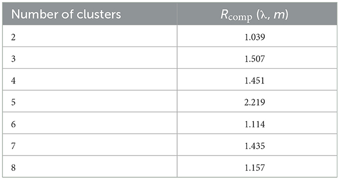
Table 2. The criterion for clustering validity of photovoltaic output curves.

The five PV output curves obtained from clustering are shown in Figure 3. The probabilities of the five scenarios appearing are 0.07, 0.25, 0.15, 0.29, and 0.24.

Figure 3

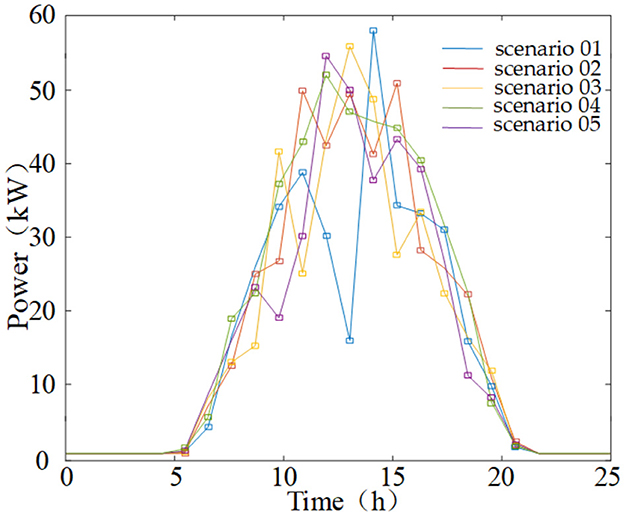
Figure 3. Photovoltaic output curve generation results.

The change in the values of the clustering validity criterion during the change in the number of clusters from 2 to 8 for the regional load scene is recorded in Table 3. According to Table 3, it is evident that when the number of categories is 5, the clustering validity criterion has the highest value. Therefore, the optimal number of categories for regional load scenarios is 5.

Table 3

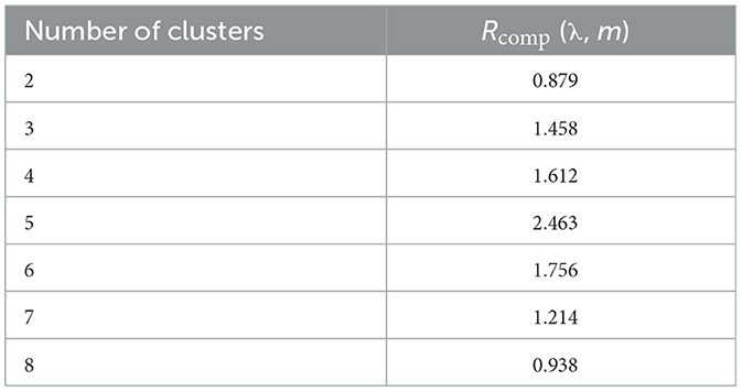
Table 3. The criterion for clustering validity of regional load curves.

The five regional load curves obtained from clustering are shown in Figure 4. The probabilities of the five scenarios appearing are 0.08, 0.14, 0.22, 0.31, and 0.25, respectively.

Figure 4

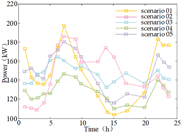
Figure 4. Regional load curve generation results.

Based on Figures 3, 4, the FCM is applied to cluster the given PV output and regional load data while preserving key characteristics such as maximum, minimum, peak, and valley values in the data set to a large extent. At the same time, the method also enhances the variability between different data sets and maximizes the uncertainty difference of power at different moments of PV output and regional loads using five scenarios.

Fifty EVs are connected to the DN. The EV charging load curve generated using the Monte Carlo method are shown in Figure 5.

Figure 5

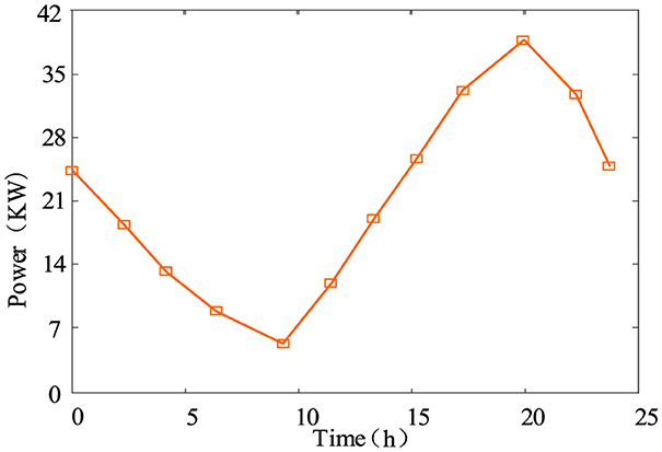
Figure 5. Electric vehicle charging load curve generation results.

According to Figure 5, EV charging has the lowest charging power around 9:00 and the highest charging power around 19:30. At least 5 EVs are charging in the DN during each time period, and up to 38 EVs are charging. The total fluctuation of the daily charging load is large.

The comprehensive load curves generated by overlying the five regional load curves in Figure 4 with the EV charging load curves in Figure 5 are shown in Figure 6.

Figure 6

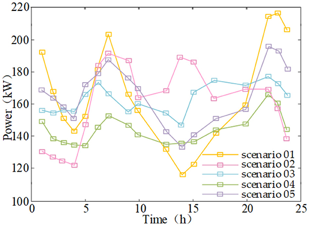
Figure 6. Comprehensive load curve generation results.

The comprehensive load curves generated by overlying the five regional load curves in Figure 4 with the EV charging load curves in Figure 5 are shown in Figure 6.

After superimposing the charging load of EVs with the five regional electricity loads, the comprehensive load curve obtained still fluctuates greatly during the day, especially in scenarios 1, 2, and 5 where the probability of occurrence is relatively low. Therefore, researching the TOU electricity pricing mechanism that adjusts dynamically based on the DN load curve is necessary.

5.2 Verification of price mechanism

5.2.1 TOU price calculation

To verify the TOU price decision model and periods division method, a simulation verification was conducted on the TOU price obtained by weighting the representative scenarios 1, 2, 4, and 5 comprehensive load curves in Figure 6. The simulation results are shown in Figure 7.

Figure 7

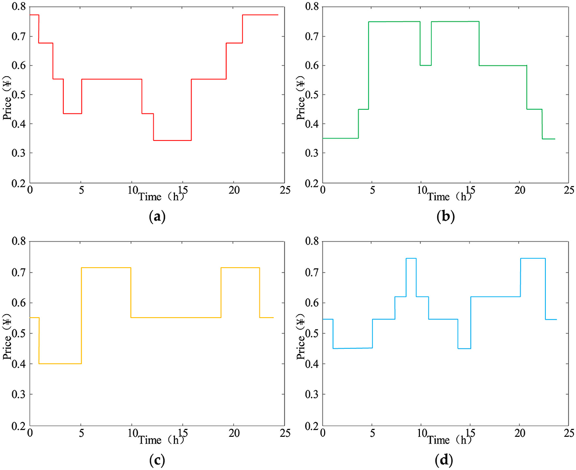
Figure 7. Time-of-use price under different load scenarios: (a) under scenario 1; (b) under scenario 2; (c) under scenario 4; (d) under comprehensive load scenario.

According to Figure 7a, under load scenario 1, due to the large peak–valley difference of the comprehensive load during the day, the TOU price calculation method divides the price into five periods. The prices are 0.335, 0.435, 0.555, 0.675, and 0.775 for the deep valley period, the valley period, the normal period, the peak period, and the sharp peak period, respectively.

According to Figure 7b, load scenario 2 has a smaller peak load during the day compared to scenario 1, and there are two peak periods for comprehensive load. The TOU price calculation method divides the price into four periods. The prices are 0.35, 0.45, 0.60, and 0.75 for the deep valley period, the valley period, the normal period, and the peak period, respectively.

According to Figure 7c, load scenario 4 has two peak periods like scenario 2, but the peak loads are smaller and the valley loads are larger. The peak-to-valley load difference is the smallest among the five scenarios. The TOU price calculation method divides the price into three periods. The prices are 0.40, 0.55, and 0.72 for the valley period, the normal period, and the peak period, respectively.

According to Figure 7d, under the five comprehensive load curves weighting scenarios, the TOU price calculation method divides the price into four periods. The prices are 0.45, 0.55, 0.625, and 0.75 for the valley period, the normal period, the peak period, and the sharp peak period, respectively.

Table 4 summarizes the time period division and TOU prices in the different scenarios. It verifies that the proposed electricity pricing mechanism can be adapted to various DN operation scenarios.

Table 4

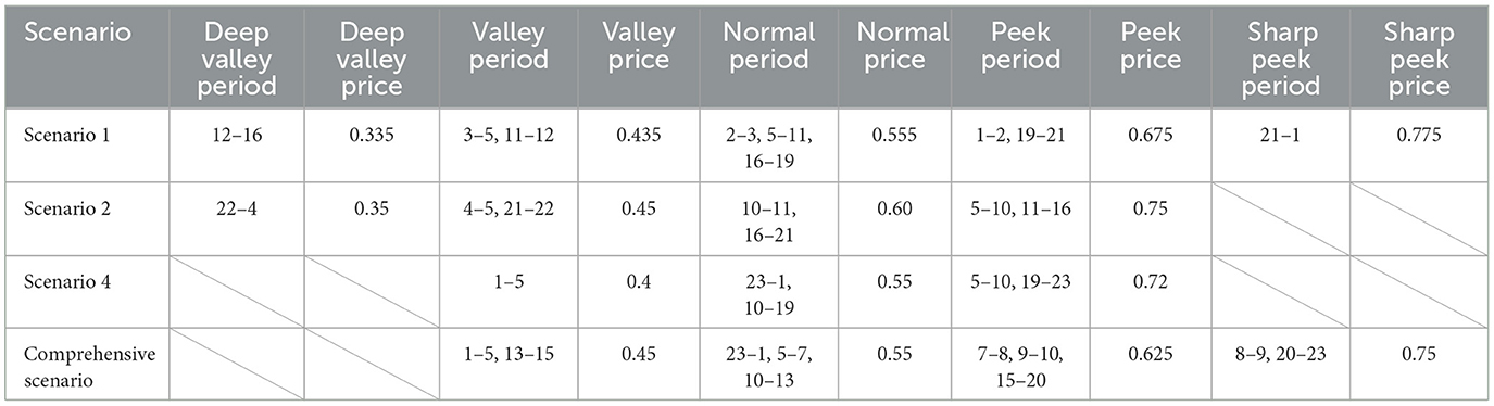
Table 4. Time division and electricity price in different scenarios.

From the preceding analysis, it is evident that the TOU price decision model and period division method presented in this article can dynamically adjust the TOU price model for different load scenarios to guide the subjects in the DN to carry out DR.

5.2.2 Comparison of TOU price mechanisms

Comparing the total peak load and peak-to-valley load, the differences between the dynamic adjustment mechanism of TOU price and the three-stage fixed price mechanism under the weighted scenario of five comprehensive load curves can be seen. The three-stage fixed prices are 0.4, 0.55, and 0.7 for the valley period, the usual period, and the peak period, respectively. The simulation results are shown in Table 5.

Table 5

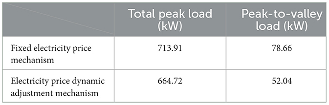
Table 5. Comparison of the scheduling effects of the two electricity price mechanisms.

According to Table 5, compared to the three-stage fixed price mechanism, the total peak load and the peak-to-valley load difference under the electricity price dynamic adjustment mechanism are both significantly reduced, which verifies the superiority of the mechanism's peak-reducing and valley-filling effects.

5.3 Verification of the scheduling model

This article takes the standard IEEE 33-node DN model as the verification scenario, which includes distributed PV, energy storage, and EVs, as shown in Figure 8. Four distributed PV devices with capacities of 500 kVA, 500 kVA, 300 kVA, and 400 kVA are connected at nodes 7, 10, 24, and 27, respectively, of the model. Two energy storage devices with capacities of 3.5 MWh and 4 MWh are connected at nodes 5 and 15, respectively. Fifty EVs are randomly connected to each node of the distribution grid for charging and discharging or DR.

Figure 8

Figure 8. Structure of the modified IEEE 33-node system.

Considering the number of EVs participating in the response and the price, the proposed EV DR scheduling strategy is validated. The case settings are as follows:

Fixed price: The three-stage fixed prices are 0.4, 0.55, and 0.7 for the valley period, the normal period, and the peak period, respectively.

TOU price: The TOU price under the comprehensive loads calculated in the previous section is used.

Case 1: The number of EVs participating in DR in the DN is 20 with a fixed price.

Case 2: The number of EVs participating in DR in the DN is 20 with the TOU price.

Case 3: The number of EVs participating in DR in the DN is 40 with a fixed price.

Case 4: The number of EVs participating in DR in the DN is 40 with the TOU price.

The results of the calculation of DN operation revenue are shown in Table 6.

Table 6

Table 6. Distribution network (DN) operation revenue under four cases.

By analyzing Table 6, it can be seen that the economic revenue of using the TOU price model is higher when the amount of EVs participating in the response remains unchanged. Under the same price model, as the amount of EVs participating in the DR increases, there is a certain degree of improvement in economic revenue. Due to the increase in the number of participating EVs in the response, the cost paid by the DN to EV users also increases, leading to a modest increase in revenue.

The calculation results of line network loss under the four cases are shown in Table 7.

Table 7

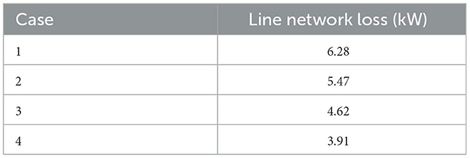
Table 7. Line network loss under four cases.

By analyzing Table 7, it can be seen that when the amount of EVs participating in the DR remains unchanged, using the TOU price model results in smaller line network loss. When using the same price model, with the amount of EVs participating in the DR increases, the line loss network decreases.

The target function values for different examples are shown in Table 8. After adopting the electricity pricing mechanism proposed in this article, the sub-values of both objective functions increased to a certain extent, verifying the effectiveness of the proposed electricity pricing mechanism in optimizing the operation of the DN compared to the fixed electricity pricing mechanism. It also indicates that as the number of EVs participating in scheduling increases, it can optimize the operating revenue and line losses of the DN.

Table 8

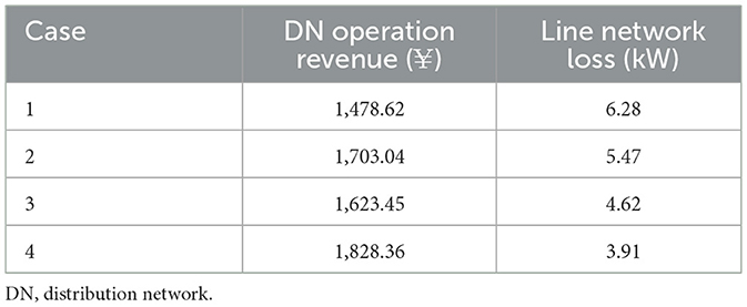
Table 8. The value of objective function in different cases.

Based on the preceding analysis, it is evident that the DR scheduling strategy for EVs constructed in this article is relatively effective in enhancing the DN's operating revenue and reducing line network losses.

CPLEX in MATLAB is used to solve the optimal scheduling model. When taking the objective function's maximum value, the scheduling results are shown in Figures 9–11.

Figure 9

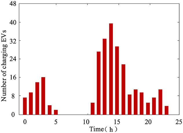
Figure 9. Number of charging electric vehicles in each period.

Figure 10

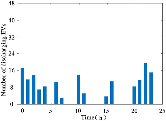
Figure 10. Number of discharging electric vehicles in each period.

Figure 11

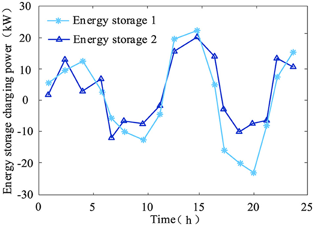
Figure 11. Charging and discharging power of two energy storages in each period.

As shown in Figure 9, after adopting the EV scheduling method proposed in this article, the number of charging EVs significantly decreased during the high comprehensive load periods of 6–10 and 17–22. This proves that the proposed EV scheduling method can alleviate the DN's power supply pressure and optimize its operation status by reducing the charging load of EVs during peak electricity consumption periods.

As shown in Figure 10, during periods of high load levels, such as 6–7, 10–11, 15–16, and 20-−22, the proposed EV scheduling method can stimulate some EVs to discharge, thereby reducing the power supply pressure on the DN and optimizing its operational status.

As shown in Figure 11, in the DR equipment scheduling model constructed in this article, two energy storage devices can adjust their charging and discharging power based on the comprehensive load curve of the DN. They discharge at 7–11 and 17–22 when the comprehensive load is high and charge at 23–6 and 12–16 when the comprehensive load is low. This proves that the DR equipment scheduling model constructed in this article can smooth the load curve of the DN and improve the operating income of the DN by controlling the energy storage devices to charge during low-load periods and discharge during high-load periods.

From Figures 9–11, it is evident that the optimization scheduling strategy can enable multiple DR resources to participate in scheduling and schedule suitable devices for DR throughout the entire period.

5.4 Summary of simulation results

This article's simulation content mainly covers displaying PV and load curve clustering results, verifying the TOU electricity price dynamic adjustment mechanism, and verifying the EV DR scheduling strategy.

The simulation part of Section 5 is based on historical PV and load data, using the FCM to extract typical PV and regional load power curves, namely, five PV scenarios and five load scenarios, and using the Monte Carlo method to generate the charging load curve of EVs. Overlaying the power curves of PV, regional load, and EVs, five comprehensive load curves, namely, five comprehensive load scenarios, are obtained.

The TOU electricity prices are calculated for the representative scenarios 1, 2, 4, and 5 comprehensive load curve weighted scenarios, and the effectiveness of the proposed TOU electricity price calculation model is verified by flexibly adjusting the number of time periods and time period electricity prices in different scenarios.

The peak total load and peak valley load differences are compared under the dynamic adjustment mechanism of TOU electricity price proposed in this article and the fixed electricity price mechanism in five weighted scenarios of comprehensive load curves. The simulation results show that compared with the latter, the peak total load and peak valley load difference of the former have decreased by 6.9% and 33.8% respectively, verifying the proposed TOU electricity price dynamic adjustment mechanism's effectiveness in peak shaving and valley filling.

To verify the proposed DR scheduling strategy's effectiveness for EVs, four examples were set up to compare and demonstrate the impact of different electricity pricing policies and the number of participating EVs on the operating revenue and line losses of the DN. The simulation results show that when participating in the response to the number of EVs, using the proposed TOU electricity price dynamic adjustment mechanism can increase the operating income of the DN by 13.2% and reduce the line loss by 12.9% compared to using a fixed electricity price. This proves the effectiveness of the DR scheduling strategy in improving the economic benefits of the DN.

6 Conclusion

To improve the DN's economic operation level by scheduling the DR resources, this article presents a DR scheduling strategy for EVs based on the dynamic adjustment mechanism of TOU price. The case analysis shows the following:

1. A scene generation clustering algorithm has been proposed and applied to cluster PV output and regional load curves in the DN. The case studies show that both PV output and regional load scenarios can be approximated by five curves.

2. The proposed dynamic adjustment mechanism of TOU price utilizing the electricity load operation curves can provide electricity price according to the operating status of the DN. Compared to implementing the fixed electricity price mechanism, the total peak load and peak–valley load difference decreased by 6.9% and 33.8%, respectively.

3. An optimal scheduling model incorporating both the operating revenue of the DN and the line network loss can be constructed. By solving the scheduling model, optimizing both the economic expense of system operation and the expense of line network loss is achieved. According to the analysis of the case simulations, it can be seen that the operating revenue of the DN can be increased by 13.2% and the line network loss can be decreased by 12.9%.

Based on the research in this article, the inclusion of distributed wind power generation, distributed generating units and other multidiscipline scheduling subjects, TOU price adjustment mechanism, and multi-objective optimal scheduling strategy under larger scale EVs access will be the focus of further research.

Data availability statement

The original contributions presented in the study are included in the article/supplementary material, further inquiries can be directed to the corresponding author.

Author contributions

YL: Conceptualization, Data curation, Investigation, Methodology, Writing – original draft, Writing – review & editing. HY: Conceptualization, Investigation, Methodology, Writing – original draft, Writing – review & editing. FW: Conceptualization, Investigation, Writing – original draft. MH: Conceptualization, Methodology, Writing – review & editing. JS: Supervision, Data curation, Writing – review & editing. WL: Project administration, Writing – review & editing. YW: Conceptualization, Writing – review & editing. LL: Methodology, Writing – review & editing. ML: Funding acquisition, Writing – review & editing.

Funding

The author(s) declare that financial support was received for the research and/or publication of this article. This work was supported by the State Grid Shandong Electric Power Company under the science and technology project “Research on hierarchical partition access control technology of large-scale distributed energy considering demand side response” (Grant No. 52062622002F). State Grid Shandong Electric Power Company was not involved in the study design, collection, analysis, interpretation of data, the writing of this article, or the decision to submit it for publication.

Conflict of interest

ML was employed by State Grid Shandong Electric Power Company.

The remaining authors declare that the research was conducted in the absence of any commercial or financial relationships that could be construed as a potential conflict of interest.

Generative AI statement

The author(s) declare that no Gen AI was used in the creation of this manuscript.

Publisher's note

All claims expressed in this article are solely those of the authors and do not necessarily represent those of their affiliated organizations, or those of the publisher, the editors and the reviewers. Any product that may be evaluated in this article, or claim that may be made by its manufacturer, is not guaranteed or endorsed by the publisher.

References

Ahsan, F., Dana, N. H., Sarker, S. K., Li, L., Muyeen, S. M., Ali, M. F., et al. (2023). Data-driven next-generation smart grid towards sustainable energy evolution: techniques and technology review. Prot. Control Mod. Power Syst. 8, 1–42. doi: 10.1186/s41601-023-00319-5

Crossref Full Text | Google Scholar

Alamolhoda, A., Ebrahimi, R., Moghaddam, M. S., and Ghanbari, M. (2024). Integrated load and energy management in active DNs featuring prosumers based on PV and energy storage systems. J. Mod. Power Syst. Clean Energy 10, 1–11. doi: 10.35833/MPCE.2023.000944

Crossref Full Text | Google Scholar

Arbelaitz, O., Gurrutxaga, I., Muguerza, J., Pérez, J. M., and Perona, I. (2013). An extensive comparative study of cluster validity indices. Pattern Recognit. 46, 243–256. doi: 10.1016/j.patcog.2012.07.021

Crossref Full Text | Google Scholar

Chaouch, M. (2013). Clustering-based improvement of nonparametric functional time series forecasting: application to intra-day household-level load curves. IEEE Trans. Smart Grid 5, 411–419. doi: 10.1109/TSG.2013.2277171

Crossref Full Text | Google Scholar

Choi, D. G., and Murali, K. (2022). The impact of heterogeneity in consumer characteristics on the design of optimal time-of-use tariffs. Energy 254:124248. doi: 10.1016/j.energy.2022.124248

Crossref Full Text | Google Scholar

Fu, X., Guo, Q., and Sun, H. (2020). Statistical machine learning model for stochastic optimal planning of DNs considering a dynamic correlation and dimension reduction. IEEE Trans. Smart Grid 11, 2904–2917. doi: 10.1109/TSG.2020.2974021

Crossref Full Text | Google Scholar

Gao, B., Zhu, Y., and Li, Y. (2023). Optimal operation strategy analysis with scenario generation method based on principal component analysis, density canopy, and K-medoids for integrated energy systems. J. Mod. Power Syst. Clean Energy 12, 89–100. doi: 10.35833/MPCE.2022.000681

Crossref Full Text | Google Scholar

Imani, M. H., Niknejad, P., and Barzegaran, M. R. (2019). Implementing time-of-use demand response program in microgrid considering energy storage unit participation and different capacities of installed wind power. Electr. Power Syst. Res. 175:105916. doi: 10.1016/j.epsr.2019.105916

Crossref Full Text | Google Scholar

Kaur, A. P., and Singh, M. (2023). Time-of-use tariff rates estimation for optimal demand-side management using electric vehicles. Energy 273:127243. doi: 10.1016/j.energy.2023.127243

Crossref Full Text | Google Scholar

Li, Y. H., Sun, Y. Y., Wang, Q. Y., Sun, K., Li, K. J., Zhang, Y., et al. (2023). Probabilistic harmonic forecasting of the distribution system considering time-varying uncertainties of the distributed energy resources and electrical loads applied. Energy 329:120298. doi: 10.1016/j.apenergy.2022.120298

Crossref Full Text | Google Scholar

Ma, S. C., Yi, B. W., and Fan, Y. (2022). Research on the valley-filling pricing for EV charging considering renewable power generation. Energy Econ. 106:105781. doi: 10.1016/j.eneco.2021.105781

Crossref Full Text | Google Scholar

Magdy, M., Elshahed, M., and Ibrahim, D. K. (2021). Enhancing PV hosting capacity using smart inverters and time of use tariffs. Iran. J. Sci. Technol. Trans. Electr. Eng. 45, 905–920. doi: 10.1007/s40998-020-00404-7

Crossref Full Text | Google Scholar

Nicolson, M. L., Fell, M. J., and Huebner, G. M. (2018). Consumer demand for time of use electricity price: a systematized review of the empirical evidence. Renew. Sustain. Energy Rev. 97, 276–289. doi: 10.1016/j.rser.2018.08.040

Crossref Full Text | Google Scholar

Pandey, A. K., Jadoun, V. K., and Sabhahit, J. N. (2022). Real-time peak valley pricing based multi-objective optimal scheduling of a virtual power plant considering renewable resources. Energies 15:5970. doi: 10.3390/en15165970

Crossref Full Text | Google Scholar

Rajabi, A., Eskandari, M., Ghadi, M. J., Li, L., Zhang, J., Siano, P., et al. (2020). A comparative study of clustering techniques for electrical load pattern segmentation. Renew. Sustain. Energy Rev. 120:109628. doi: 10.1016/j.rser.2019.109628

Crossref Full Text | Google Scholar

Rao, Y. Q., Yang, J., Xiao, J. X., Xu, B., Liu, W., Li, Y., et al. (2021). A frequency control strategy for multimicrogrids with V2G based on the improved robust model predictive control. Energy 222:119963. doi: 10.1016/j.energy.2021.119963

Crossref Full Text | Google Scholar

Ren, H., Tseng, C. L., Wen, F., Wang, C., Chen, G., Scenario-Based Optimal, L., et al. (2024). Real-time charging strategy of electric vehicles with Bayesian long short-term memory networks. J. Mod. Power Syst. Clean Energy 12, 1572–1583. doi: 10.35833/MPCE.2023.000512

Crossref Full Text | Google Scholar

Satre-Meloy, A., Diakonova, M., and Grünewald, P. (2020). Cluster analysis and prediction of residential peak demand profiles using occupant activity data. Appl. Energy 260:114246. doi: 10.1016/j.apenergy.2019.114246

Crossref Full Text | Google Scholar

Shabbir, N., Kütt, L., Astapov, V., Daniel, K., Jawad, M., Husev, O., et al. (2024). Enhancing PV hosting capacity and mitigating congestion in DNs with deep learning based PV forecasting and battery management. Appl. Energy 372:123770. doi: 10.1016/j.apenergy.2024.123770

Crossref Full Text | Google Scholar

Shan, P. B., Sun, Y. Y., Song, Y. Z., Zhang, F., Li, Y., Sun, K., et al. (2025). Adaptive parameter tuning and virtual impedance injection control for coupled harmonic mitigation of photovoltaic converter. IEEE Trans. Power Electron 40, 162–175. doi: 10.1109/TPEL.2024.3449080

Crossref Full Text | Google Scholar

Song, Y., Liu, S. G., and Li, G. (2021). Simulation analysis of flexible concession period contracts in electric vehicle charging infrastructure public-private-partnership (EVCI-PPP) projects based on time-of-use (TOU) charging price strategy. Energy 228:120328. doi: 10.1016/j.energy.2021.120328

Crossref Full Text | Google Scholar

Sun, Y. Y., Xu, Q. S., and Ma, Z. (2024). Key technologies for harmonic source tracing in new power system in background of digitalization. Autom. Electr. Power Syst. 48, 154–169. doi: 10.7500/AEPS20230613002

Crossref Full Text | Google Scholar

Venizelou, V., Philippou, N., Hadjipanayi, M., Makrides, G., Efthymiou, V., Georghiou, G. E., et al. (2018). Development of a novel time-of-use tariff algorithm for residential prosumer price-based demand side management. Energy 142, 633–646. doi: 10.1016/j.energy.2017.10.068

Crossref Full Text | Google Scholar

Wang, H. Y., Wang, J. S., and Wang, G. (2022). A survey of fuzzy clustering validity evaluation methods. Inf. Sci. 618, 270–297. doi: 10.1016/j.ins.2022.11.010

Crossref Full Text | Google Scholar

Wang, Y., Qiu, D., Strbac, G., and Gao, Z. (2023). Coordinated electric vehicle active and reactive power control for active DNs. IEEE Trans. Ind. Informat. 19, 1611–1622. doi: 10.1109/TII.2022.3169975

Crossref Full Text | Google Scholar

Xu, H., Feng, B., Wang, C., Guo, C., Qiu, J., Sun, M., et al. (2023). Exact box-constrained economic operating region for power grids considering renewable energy sources. J. Mod. Power Syst. Clean Energy 12, 514–523. doi: 10.35833/MPCE.2023.000312

Crossref Full Text | Google Scholar

Xue, W., Zhao, X., Li, Y., Mu, Y., Tan, H., Jia, Y., et al. (2023). Research on the optimal design of seasonal time-of-use tariff based on the price elasticity of electricity demand. Energies 16:1625. doi: 10.3390/en16041625

Crossref Full Text | Google Scholar

Yang, B., Zheng, R., Han, Y., Huang, J., Li, M., Shu, H., et al. (2024). Recent advances in fault diagnosis techniques for photovoltaic systems: a critical review. Prot. Control Mod. Power Syst. 9, 36–59. doi: 10.23919/PCMP.2023.000583

Crossref Full Text | Google Scholar

Yang, H., Gong, Z., Ma, Y., Wang, L., and Dong, B. (2020). Optimal two-stage dispatch method of household PV-BESS integrated generation system under time-of-use electricity price. Int. J. Electr. Power Energy Syst. 123, 106244. doi: 10.1016/j.ijepes.2020.106244

Crossref Full Text | Google Scholar

Yang, L., Dong, C., Wan, C. L. J., and Ng, C. T. (2013). Electricity time-of-use tariff with consumer behavior consideration. Int. J. Prod. Econ. 146, 402–410. doi: 10.1016/j.ijpe.2013.03.006

Crossref Full Text | Google Scholar

Yang, Z., Trivedi, A., Ni, M., Liu, H., and Srinivasan, D. (2023). Distribution locational marginal pricing based equilibrium optimization strategy for data center park with spatial-temporal demand-side resources. J. Mod. Power Syst. Clean Energy 11, 1959–1970. doi: 10.35833/MPCE.2022.000450

Crossref Full Text | Google Scholar

Yin, S. L., Sun, Y. Y., Xu, Q., Sun, K., Li, Y., Ding, L., et al. (2024). Multi-harmonic sources identification and evaluation method based on cloud-edge-end collaboration. Int. J. Electr. Power Energy Syst. 156:109681. doi: 10.1016/j.ijepes.2023.109681

Crossref Full Text | Google Scholar

Yin, W. J., Wen, T., and Zhang, C. (2023). Cooperative optimal scheduling strategy of electric vehicles based on dynamic electricity price mechanism. Energy 263:125627. doi: 10.1016/j.energy.2022.125627

Crossref Full Text | Google Scholar

Zhang, H., Tian, Y., He, W., Liang, Z., Zhang, Z., Zhang, N., et al. (2025). The generation load aggregator participates in the electricity purchase and sale strategy of the electric energy–peak shaving market. Energies 18:370. doi: 10.3390/en18020370

Crossref Full Text | Google Scholar

Zhang, J., Yan, J., Liu, Y., Zhang, H., and Lv, G. (2020). Daily electric vehicle charging load profiles considering demographics of vehicle users. Appl. Energy 274:115063. doi: 10.1016/j.apenergy.2020.115063

Crossref Full Text | Google Scholar

Zhang, Y., Wang, W., Zhang, X., and Li, Y. (2008). A cluster validity index for fuzzy clustering. Inf. Sci. 178, 1205–1218. doi: 10.1016/j.ins.2007.10.004

Crossref Full Text | Google Scholar

Zhou, K., Cheng, L., Lu, X., and Wen, L. (2020). Scheduling model of electric vehicles charging considering inconvenience and dynamic electricity prices. Appl. Energy 276:115455. doi: 10.1016/j.apenergy.2020.115455

Crossref Full Text | Google Scholar

Zhu, X., Li, L., Zhou, K., and Yang, S. (2018). A meta-analysis on the price elasticity and income elasticity of residential electricity demand. J. Clean. Prod. 201, 169–177. doi: 10.1016/j.jclepro.2018.08.027

Crossref Full Text | Google Scholar