Circular Path and Linear Momentum Method for Seismic Response Analysis of Vehicles

Introduction

Driving a vehicle during a strong earthquake can lead to a serious accident if the driver loses control, which can happen even in a moderate-level earthquake when the driver does not feel the ground motion. Although earthquake damage to roads and infrastructure can be reduced by strengthening structures and increasing their earthquake resilience, lowering the risk of a vehicle driver losing control during a strong earthquake is more complex, involving mechanical, physical, and psychological factors. This risk depends on the individual’s driving skills, physical and psychological abilities, and on the mechanical properties of the vehicle.

The effect of an earthquake on the driver of a moving vehicle during an earthquake may be negligible when the ground motion is small, as the vehicle itself is in motion. However, large shaking may push the vehicle laterally or longitudinally, causing the driver to lose control of the vehicle. Drivers’ responses and the characteristics of ground motions during the 1983 M7.7 Nihon-kai-chubu earthquake in Akita Prefecture and the 1987 M6.7 Chiba-ken-oki earthquake in Chiba Prefecture, which both resulted in Japan Meteorological Agency (JMA) seismic intensities of V (JMA, 1996), were surveyed using a questionnaire (Kawashima et al., 1989). The survey revealed that about 50% of drivers felt the earthquake motion as the vehicle and their surroundings displayed unusual behavior and movement. Most of the drivers stopped their vehicles (65 and 43.3% in the 1983 and 1987 events, respectively) because they felt they were in danger. The survey also found that steering instability was felt in directions both longitudinally and laterally to the car while driving the vehicles (73.8 and 52.4%, respectively). A similar study following the 2003 M7.0 Miyagiken-Oki earthquake found a relationship between the JMA intensity of the earthquake and the drivers’ recognition of the event and their driving response to it (Maruyama and Yamazaki, 2006). Only 40% of the drivers recognized earthquakes of JMA intensity less than 4.0, but more than 80% noticed and most of them reacted when the intensity was larger than 4.0. For JMA intensities larger than 4.5, 20% of the drivers stopped on the shoulders of the roads.

Maruyama and Yamazaki (2002) studied the response of a moving vehicle to earthquake motion with various JMA intensities, where the vehicle was modeled with six degrees of freedom. That model used the equation of motion with a constant longitudinal speed. The vehicle drift for four earthquakes (Kobe, El Centro, Tottori and Chiba-ken-oki) was mostly unidirectional and linear. However, this model could not provide a good simulation of the behavior of the vehicle at rest. Hence, we propose a new method of seismic response analysis: the “circular path and linear momentum” (CPLM) method for the lateral and longitudinal stability analysis of vehicles both in motion and at rest. We compare the result with the response of a vehicle at rest just before the shaking of the Gorkha 2015 earthquake.

To analyse the vehicle’s response to seismic motion, the vehicle was modeled with six degrees of freedom. The equation of motion was used as the basic equation for the analysis of the response of the tires and the car body as well as the transformation of the acceleration from the road surface to the vehicle. The longitudinal and lateral responses were calculated using the CPLM method. We also considered the pitching, rolling, and yawing motions of the vehicle as rotations in three directions. The forces acting on the tires were calculated using the Magic Formula Model (MFM) (Pacejka, 2006). The MFM coefficients were taken from previously published results (Alagappan et al., 2014) using the trust region reflective (TRR) method algorithm. We analyzed the responses of a car, bus, and truck in the longitudinal and lateral directions for several conditions. The relationships between the vehicles’ responses with speeds of up to 30.0 m/s from rest condition and peak ground acceleration (PGA) from 1.0 to 15.0 m/s² were also investigated.

The CPLM Method

The seismic response of a vehicle is different from the response of a structure that is fixed to the ground; in the case of a vehicle, the tires roll on the ground as forces act on them. As a force is applied to a vehicle, friction produces resistance to the lateral movement, which differs from the resistance in the direction in which the vehicle is moving. Rolling friction is the force required to overcome the resistance between the tire and the road surface while at rest to initiate the rolling movement of the wheel; this is a relatively small quantity compared with the friction between the rubber tire and the road surface. When a vehicle is at rest, without applying the hand brake and in neutral gear, the longitudinal force needed to move the car forward is equal to a force that is slightly more than the rolling frictional force that acts in the opposite direction to the applied force. When a vehicle wheel starts to roll, it will acquire linear momentum from the speed that the vehicle develops.

When a lateral force acts on a vehicle at rest, the vehicle may remain at rest or move sideways. If the frictional force is sufficiently high, the vehicle will not move; however, if the lateral force exceeds the frictional force the vehicle will shift laterally. The lateral movement will depend on the amplitude of the resultant force. In the case of a moving vehicle, the lateral force acts for a very short time, pushing the vehicle from the side. As a result, the vehicle’s path will bend, forming a curve during that time interval.

To simulate lateral forces on a moving vehicle, the CPLM method assumes that the earthquake forces in each time interval push the vehicle body in a lateral direction, acting as a centripetal force exerted on the vehicle as it moves in a circular path. The lateral force varies with time as the earthquake force changes not only in direction but also in magnitude. The variation of the lateral force in each time step determines the radius of the arc that defines the vehicle path in each time interval. Changes in the radius and center of rotation of a moving vehicle under earthquake loading can be described by the kinematics of a turning vehicle considering moving centrodes (Guiggiani, 2014). Hence, the direction in which the vehicle moves during each step is determined by the relation between the length and the radius of the arc. The length of the arc can be calculated from the speed of the vehicle at that time step. The absolute direction of the vehicle can be determined from the accumulation of angular deviation in each time step for that arc. The position of the vehicle in each time step is derived using the principle of conservation of linear momentum. The force acting in the longitudinal direction is the external force applied at a particular time, changing the momentum, and producing the vehicle velocity that is used in the next step of the modeling. Hence, by integrating the concept of the centripetal force acting on a vehicle moving along a circular arc and the principle of linear momentum we obtain the position of the vehicle during an earthquake. Figure 1 shows a schematic diagram of the vehicle movements considered in each time step of the calculation. We set the absolute coordinate system X and Y in the longitudinal and lateral directions; t₀, t₁, t₂, t₃, … where t_n−1 and t_n are the time intervals for the calculation, v is the velocity vector, and F_x and F_y are longitudinal and lateral forces that act on the vehicle, respectively. The line: “o–l” is parallel to the absolute longitudinal axis, where “o–x” represents the local longitudinal axis and “o–a” represents the line parallel to the local longitudinal axis of the vehicle in the previous step.

FIGURE 1

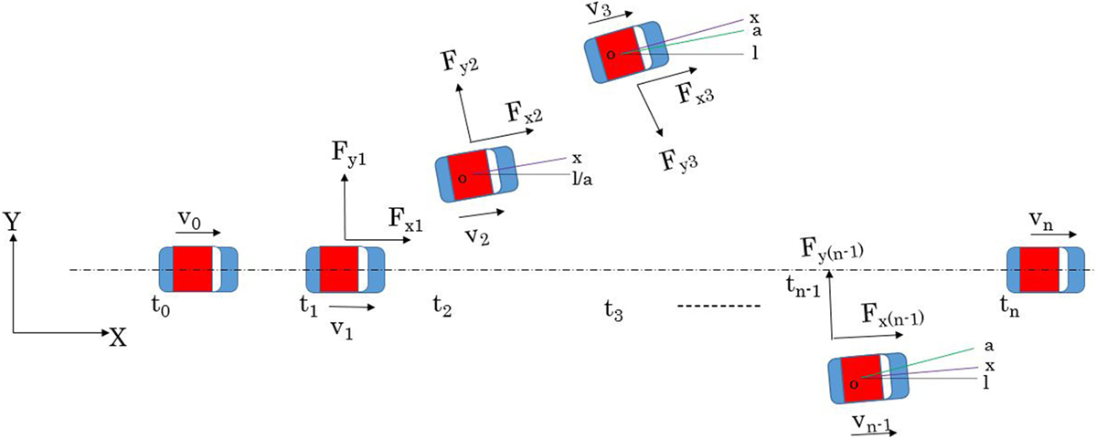
Figure 1. Schematic diagram of vehicle positions, axes, and forces.

Vehicle Model

Each vehicle model is defined by a system with six degrees of freedom consisting of three translational and three rotational motions. The longitudinal, lateral, and vertical translational motions, as well as the corresponding rotational motions – roll, pitch, and yaw – along the X, Y, and Z axes, are shown in Figure 2 along with dimensional parameters. The vehicle model parameters were obtained for a HONDA CIVIC car, a HINO SELEGA_R GD bus, and a HINO PROFIA CARGO FR truck. All of these double-axle vehicles are assumed to be running in dry road conditions for this study. The mass of the vehicle bodies and tires, vehicle dimensions, and other parameters for the three vehicle types are shown in Table 1.

FIGURE 2

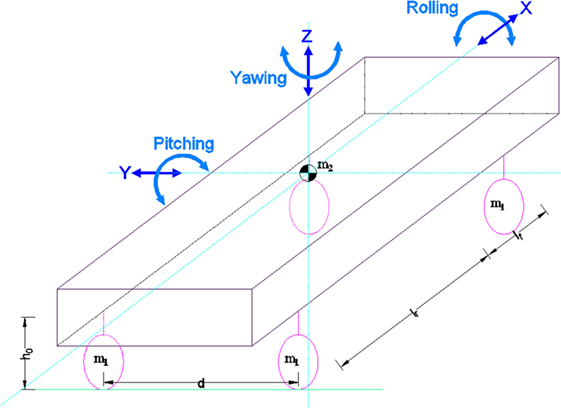
Figure 2. Vehicle model and basic motions of the vehicle.

TABLE 1

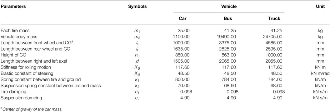
Table 1. Parameters of the vehicle models.

Seismic Response Analysis

The rolling and pitching motions of the vehicle are the rotational motions about the longitudinal and lateral axes, respectively. Taking the moments of the forces acting on those axes, the relationships of the forces are as shown,

$\left(K_{\varnothing }-\mathit{mgh}\right)\varnothing =m\left(\dot{v}+\mathit{ur}\right)h$ (1)

$\left\{2K\left(l_f^2+l_r^2\right)\right\}{\mathrm{\theta }}_p=m\left(\dot{u}-\mathit{vr}\right)h$ (2)

where m is the mass of the vehicle, K_∅ is the rolling stiffness, K is the stiffness of the tire, ∅ is the rolling angle, θ_p is the pitching angle, h is the height of the center of gravity (CG) of the vehicle mass, and u and v are the longitudinal and lateral velocities of the vehicle, respectively. The yaw angular velocity is denoted by r, and l_f and l_r are the distances of the front and rear axle from the CG of the vehicle mass, respectively.

The yawing motion of the vehicle is the remaining rotational motion about the vertical axis, and can be described by Eq. 3, where I_z is the moment of inertia of the vehicle, d is the distance between the right and left wheels, and $F_y^{\prime }$ and $F_x^{\prime }$ are the lateral and longitudinal forces acting on each tire, respectively (indices 1 and 2 refer to the front and rear and left and right, respectively).

$\begin{array}{ll}\hfill I_z\frac{\mathit{dr}}{\mathit{dt}}& =\left(F_{y11}^{\prime }+F_{y12}^{\prime }\right)l_f-\left(F_{y21}^{\prime }+F_{y22}^{\prime }\right)l_r+\left(-F_{x11}^{\prime }+F_{x12}^{\prime }\right)\frac{d}{2}+\left(-F_{x21}^{\prime }+F_{x22}^{\prime }\right)\frac{d}{2}\end{array}$ (3)

The vertical response of the modeled vehicle to earthquake excitation is defined using a two degrees-of-freedom system. The representation of the road, tire, and car body using springs and dashpots as a quarter vehicle model (Figure 3) is used in this study. Each tire is represented by a mass (m₁) and a spring and dashpot (k₁ and c₁) connected to the ground, and the vehicle is modeled as a mass (m₂) and a spring and dashpot (k₂ and c₂) over the axle (vehicle suspension). Equations 4 and 5 are the equations of motion for the model, where z_g is the vertical displacement of the ground, and z₁ and z₂ are the relative vertical displacements of the tire and vehicle body, respectively.

$m_1\left({\ddot{z}}_1+{\ddot{z}}_g\right)+c_1{ż}_1+c_2\left({ż}_1-{ż}_2\right)+k_1{z}_1+k_2\left(z_1-z_2\right)=0$ (4)

$m_2\left({\ddot{z}}_2+{\ddot{z}}_g\right)+c_2\left({ż}_2-{ż}_1\right)+k_2\left(z_2-z_1\right)=0$ (5)

FIGURE 3

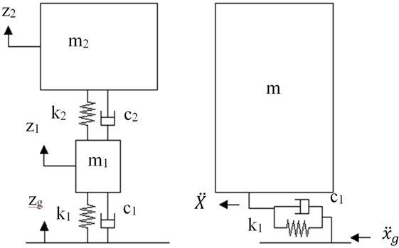
Figure 3. Free body diagram of the quarter-vehicle model for deriving the vertical response of a vehicle (left panel) and single degree-of-freedom system of the ground and vehicle for modeling the lateral acceleration transfer (right panel).

The transformation of the ground acceleration to the vehicle in the longitudinal and transverse directions can be modeled using a single degree-of-freedom system that comprises the ground and the car body. The stiffness and damping constants used for the tire properties in the vertical response analysis were used for the lateral acceleration calculation (Eqs 6 and 7). ${\ddot{x}}_g$ and ${\ddot{y}}_g$ are the ground accelerations and $\ddot{X}$ and $\ddot{Y}$ are the accelerations transferred to the vehicle.

$m\ddot{X}+{\text{c}}_1\dot{X}+{\text{k}}_{1}X=-m{\ddot{x}}_g$ (6)

$m\ddot{Y}+{\text{c}}_1\dot{Y}+{\text{k}}_{1}Y=-m{\dot{y}}_g$ (7)

The external forces acting on the vehicle body are now determined using the transferred accelerations after transferring the parameters from a global coordinate system to the local coordinate system. First, we obtain the absolute acceleration vector acting on the vehicle using Eqs 8–12, where a and θ_a are the magnitude and direction of the acceleration vector, and $ẍ$ and $ÿ$ are the acceleration vectors along the longitudinal and lateral axes of the vehicle in the local coordinate system. θ_l is the angle of the longitudinal axis relative to the global axis (∠lox in Figure 1), and θ_f defines the position of the acceleration vector relative to the local axis.

$a=\sqrt{{\ddot{X}}^2+{\ddot{Y}}^2}$ (8)

${\mathrm{\theta }}_{\text{a}}={\tan }^{-1}\frac{\ddot{Y}}{\ddot{X}}$ (9)

${\mathrm{\theta }}_f={\mathrm{\theta }}_a-{\mathrm{\theta }}_l$ (10)

$\ddot{x}=\ddot{\text{a}}\cos {\mathrm{\theta }}_f$ (11)

$\ddot{y}=\ddot{\text{a}}\sin {\mathrm{\theta }}_f$ (12)

We consider a vehicle moving in a circular trajectory with lateral force acting on it. This force is the sum of all the external forces in terms of the acceleration and the rotational movement of the body. The rolling of the vehicle body also exerts some lateral force, which depends on the roll angle during each step. We assume that there is no rolling motion in the first step of the analysis. In the next step, as the lateral force is activated, the vehicle begins to rock. The orientation of vehicle will begin to change as the vehicle starts to move longitudinally while the lateral force is acting on it.

The longitudinal forces acting on the vehicle are: (1) the external force exerted by the earthquake acceleration, (2) the force generated by the slip of the tires on the ground and (3) the rolling resistance of the tires. The rolling resistance force (F_roll) represents the resistance that should be overcome by the applied force to initiate the vehicle motion. In this study, for the cases with constant vehicle speed, we neglect the rolling resistance and assume constant acceleration to nullify this effect. In cases where the vehicle decelerates and stops or where the vehicle is at rest, the rolling resistance is included in the analysis.

$F_{\text{roll}}=C_{\text{roll}}\mathit{mg},$ (13)

where g is the gravitational acceleration.

The coefficients of rolling resistance (C_roll) for various vehicles moving on concrete and asphalt road surfaces are shown in Table 2 (Wong, 2001).

TABLE 2

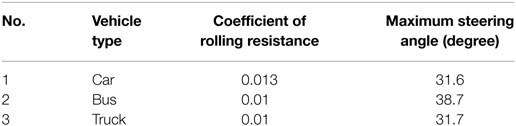
Table 2. Rolling resistance coefficients for various vehicles.

Tire slipping occurs when the speed of the vehicle is either faster or slower than the speed of the rolling tire. Here, we calculate the maximum acceleration that can be applied to the vehicle for the non-slip condition.

For a tire with radius “R” and total mass concentrated on a single tire “m_t,” when “F_rt” is the frictional force between the tire and the road surface, “I” is the angular moment of inertia about the center of the tire and “α” is the angular acceleration of the tire, then equating the angular and linear moment about the center of the wheel gives

$F_{\mathit{rt}}R=I\mathrm{\alpha }$ (14)

where the angular moment of inertia $I=\frac{1}{2}{m}_t{R}^2$, the angular acceleration $\mathrm{\alpha }=\frac{a}{R}$, and the frictional force $F_{\mathit{rt}}=\mathrm{\mu }{m}_{t}g$. “a” is the linear acceleration and “μ” is the frictional coefficient. The above relationships show that the maximum acceleration that can roll the tire without slip a_max is 2 μg. The frictional coefficient between the tires and dry asphalt concrete are taken as 0.8 (Li et al., 2015). When the applied acceleration or deceleration is larger than a_max the slip can be calculated and represented as the slip ratio,

$\text{Slip}\text{ratio}=\frac{v_2-v_a}{v_2}$ (15)

where “v₂” is the resultant velocity considering the input acceleration and “v _a” is the velocity considering the maximum acceleration. We use the MFM to calculate the longitudinal force (F_xs) acting on the tires due to the slip.

The lateral movement of the vehicle depends on the lateral force applied on the vehicle body. The slip angle “θ” determines the trajectory of the vehicle subjected to a lateral load. To calculate the slip angle, we use the centripetal force that moves the vehicle in a circular path, as described in Section “CPLM Methods.”

The centripetal force that acts on a vehicle body moving in a circular path is given by

$F_c=\frac{m{v}^2}{R_p}$ (16)

where “R_p” is the radius of the circular path, and “v” is the velocity of the vehicle.

Again, the lateral force acting on the vehicle is the sum of the external forces caused by lateral acceleration and the force generated by the rotational motion about the longitudinal axis (rolling):

$F_c=m{ÿ}_l+\mathit{mg}\text{\hspace{0.17em}sin\hspace{0.17em}}\left(\varnothing \right)$ (17)

The radius of the circular path for each time interval (R_p) can be derived from Eqs 16 and 17. The subtended angle θ for that arc can be calculated using Eq. 18, where “D” is the distance traveled by the vehicle during the time interval dt as shown in Eq. 19.

$\mathrm{\theta }={\tan }^{-1}\frac{D}{R_p}$ (18)

$D=\mathit{vdt}$ (19)

The slip angle (Eq. 18) is calculated using the radius from the CG of the vehicle to the center of the circular path. Taking into account, the variation of the radius for the left and right tires, the slip angles for the left and right front tires “${\mathrm{\theta }}_{\mathit{lt}}$” and “${\mathrm{\theta }}_{\mathit{rt}}$” can be derived from Eqs 20 and 21, respectively. The rear tires are aligned with the vehicle body; therefore, we assume zero slip angles for the rear tires. The tires do not allow the vehicle to turn in a full circle; the maximum value of the turning angle or the slip angle is assumed to be the same as that used in the geometric design of highways and roads by the American Association of State Highways and Transportation Officials (AASTHO, 2001).

${\mathrm{\theta }}_{\mathit{lt}}={\tan }^{-1}\frac{D}{R_p-\frac{d}{2}}$ (20)

${\mathrm{\theta }}_{\mathit{rt}}={\tan }^{-1}\frac{D}{R_p+\frac{d}{2}}$ (21)

The longitudinal and transverse forces acting on each tire along with the self-aligning moment are calculated using the MFM (Eqs 22–24) considering pure slip conditions.

$y\left(x\right)=D\sin \left[C\arctan \left\{\mathit{Bx}-E\left(\mathit{Bx}-\arctan \left(\mathit{bx}\right)\right)\right\}\right]$ (22)

$Y\left(x\right)=y\left(x\right)+S_v$ (23)

$x=X+S_h$ (24)

where X is the input variable: the slip angle θ and the slip ratio (Eq. 15). Y is the output variable. B, C, D, and E are the stiffness factor, shape factor, peak value, and curvature factor, respectively. These factors are calculated for pure slip conditions based on the TRR algorithm, which showed the best performance compared with other algorithms. The coefficients used to calculate the MFM parameters are shown in Table 3 (Alagappan et al., 2014). The pressure on the tires is calculated considering the static pressure as well as the effects of the rolling, pitching, and vertical motion of the vehicle (Maruyama and Yamazaki, 2002).

TABLE 3

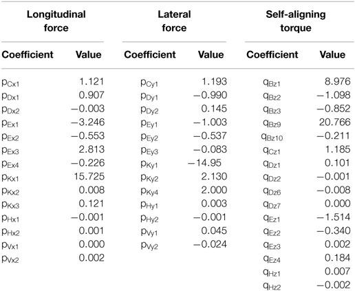
Table 3. Coefficients used to calculate the MFM parameters.

Figures 4A,B shows the variation of the longitudinal and lateral forces for a range of tire slip ratios and slip angles, respectively, for three cases of vertical loading (5.88, 3.92, and 1.96 kN). Figure 4C shows the variation of the self-aligning torque with slip angles for the same cases. We selected an R15 tire, where the nominal load is taken as 6.15 kN for calculation of MFM parameters (Alagappan et al., 2014).

FIGURE 4

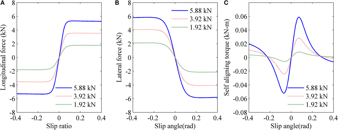
Figure 4. Relationship of (A) Longitudinal Force with slip ratio (B) Lateral force with slip angle and (C) self aligning torque with slip angle using MFM.

The total longitudinal force acting on the tire can be calculated using Eq. 25. F_roll will always act against the moving direction. F_xg is the external force from the earthquake acceleration in the longitudinal direction.

$F_x=F_{\mathit{xg}}+F_{\mathit{xs}}\pm F_{\text{roll}}$ (25)

$F_{\mathit{xg}}=m\ddot{x}$ (26)

Lateral sliding of the tires will occur when the total force acting in the lateral direction is higher than a threshold value. This value depends on the frictional force (F_r) that acts against the applied force; it is a factor of the frictional coefficient and the normal load. If the lateral force F_yg exerted on the tires due to the earthquake is larger than the frictional resistance, the vehicle will slide laterally. Here, we consider the forces that act on the tire and the road surface (Eq. 27).

$F_y=\mathrm{|}{F}_{\mathit{yg}}\mathrm{|}-F_r$ (27)

$F_{\mathit{yg}}=m\ddot{y}$ (28)

Considering the principle of conservation of momentum along the vehicle axis, we can obtain a new velocity vector $v_2$ along that axis from Eq. 29. $F_x$ is the total external force applied during the time interval (dt) in this system.

$\mathit{mv}+F_x\mathit{dt}=m{v}_2$ (29)

$v_x=v_2\cos {\mathrm{\theta }}_1$ (30)

$v_y=\left[v_2+\frac{F_y\mathit{dt}}{m}\right]\sin {\mathrm{\theta }}_1$ (31)

${{\mathrm{\theta }}_1}_1={\mathrm{\theta }}_l+\mathrm{\theta }$ (32)

${\mathrm{\theta }}_{1_{i+1}}={\mathrm{\theta }}_{1_i}+{\mathrm{\theta }}_{i+1}$ (33)

$D_{x_i}=D_{x_{i-1}}+v_{x_i}\mathit{dt}$ (34)

$D_{y_i}=D_{y_{i-1}}+v_{y_i}\mathit{dt}$ (35)

The velocity and displacement of the vehicle are now calculated from Eqs (30–34) in global coordinates. The path of the vehicle in each step is determined by summing the slip angles using Eq. (35).

Validation of the Model

The Gorkha earthquake in Nepal was one of the largest earthquakes of 2015 and is noted for the unique nature of its ground motion. The ground motion recorded in Kathmandu had a long period and shook central Nepal severely even though the PGA was relatively low (Parajuli and Kiyono, 2015). The Nepali police released several closed-circuit television (CCTV) videos (Video 1 in Supplementary Material) after the earthquake that recorded the shaking in the streets of Kathmandu. For our study, we used one of these videos that captured the vehicle response during the earthquake in Sundhara, one of the major public transport hubs in Kathmandu.

The video shows a minibus that stopped just before the earthquake struck, with passengers getting out of the vehicle while others are trying to get in (circled in yellow, Figure 5). When the shaking starts people panic, the door moves and some people get out of the vehicle during the shaking. To track the position of the minibus, we picked its location in the photo frame every 0.2 s. We also established a baseline in reference to a stiff object nearby to correct for the effect of shaking. We then compared the vehicle motion during the earthquake derived from the video to the seismic response of the modeled vehicle using the CPLM method. The orientation of the vehicle is N14° 30′E, calculated using two points along with the reference to the road side, which has a bearing of N3° 30′E (Figure 5). The vehicle is a Toyota HiAce and the dimensions and weight parameters are taken from the Toyota specification sheet (Toyota, 2015). The wheelbase of the vehicle is 2.57 m; the distance between the right and left wheels is 1.47 m and the curb weight is 1825 kg. We assumed that the CG of the vehicle is in the center of the wheelbase; the other parameters are listed in Table 1.

FIGURE 5

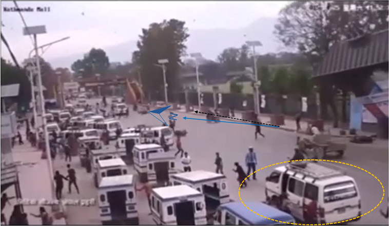
Figure 5. Photo frame from a CCTV video recorded in Sundhara. The orientation of the road (dashed black and solid blue lines) and the modeled vehicle (dashed yellow circle) are shown.

As the vehicle was oriented toward the northeast, we used the N–S component of the ground motion as the longitudinal axis and the E–W component as the lateral direction of the vehicle. We used the Gorkha earthquake data recorded at the US Geological Survey’s KATNP station (USGS, 2015), 1.2 km from the location of the video camera. The ground motion records and corresponding response spectra, considering 5% damping, are shown in Figure 6. The orientation of the vehicle is also used in the analysis. The results showing the longitudinal and lateral displacements of the vehicle in response to the earthquake motion are shown in Figure 7 for the CPLM method and the video analysis. The two response curves are well matched. Note that the video shows that people were getting on and off the bus, and the driver initially may have used the brakes; these are factors that are not accounted for in the numerical simulation. Moreover, considering that the alignment of the vehicle during the shaking may be different, its resulting response may vary, depending on the angle of orientation that we discuss later with results shown in Figure 14.

FIGURE 6

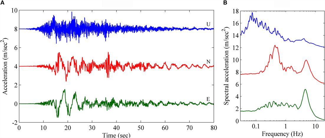
Figure 6. Gorkha earthquake ground motion parameters. (A) Acceleration and (B) response spectra.

FIGURE 7

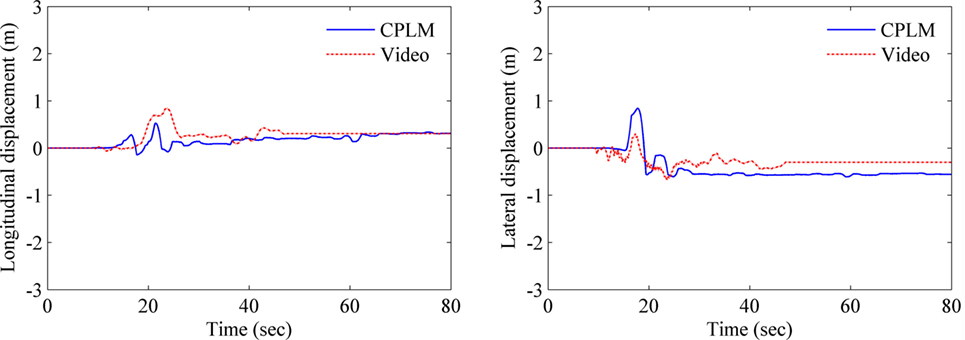
Figure 7. Comparison of the seismic response of the vehicle using the CPLM method and analysis of video footage of the shaking vehicle during the Gorkha earthquake.

Results and Discussion

The vehicle seismic response analyzes were performed in ideal situations that considered the movement of the vehicle without any responsive actions from the driver. We chose 10 earthquake datasets from around the globe (Table 4) with moment magnitudes of 6.7–9.0. The selected earthquakes occurred between 1940 and 2015. The PGA in the E–W direction varied between 1.54 m/s² for the Gorkha earthquake and 17.40 m/s² for the Northridge earthquake. In the N–S direction, the minimum and maximum PGAs were 1.60 and 25.9 m/s² for the Gorkha and Great East Japan earthquakes, respectively. The N–S components for all the earthquake records are shown in Figure 8 along with corresponding Fourier spectra. The ground acceleration data-sampling rate varied from 50 to 200 Hz; for consistency, we selected all the data sampled at 50 Hz for analysis. The displacement time series of all the earthquakes (Figure 9) were calculated using Newmark’s integration method.

TABLE 4

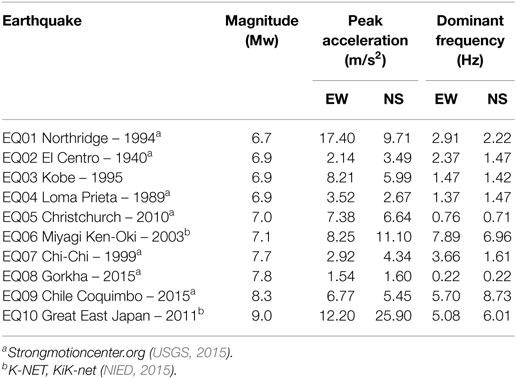
Table 4. List of earthquake datasets used in the analysis.

FIGURE 8

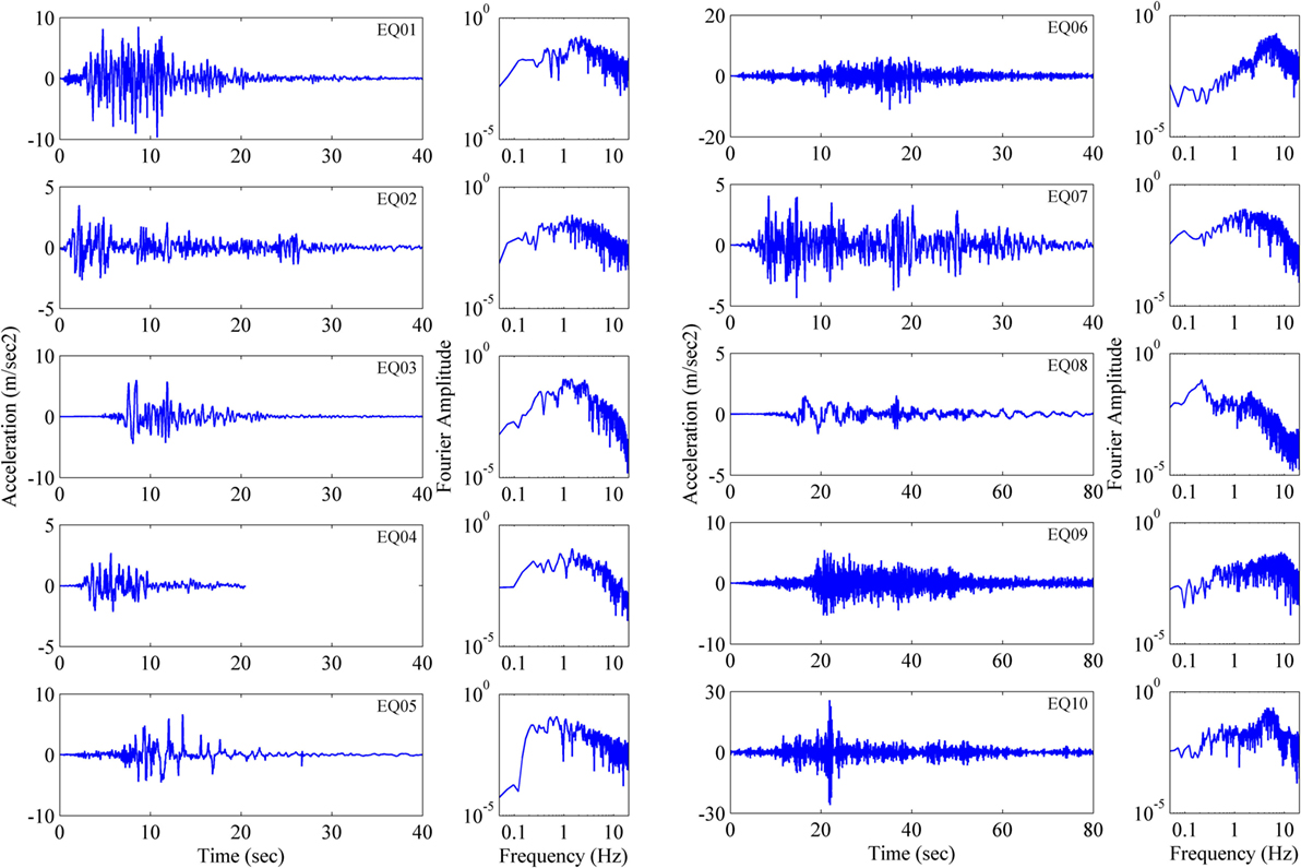
Figure 8. N–S components of the recorded ground motions (first and third columns) and corresponding Fourier spectrums (second and fourth columns) of selected earthquakes.

FIGURE 9

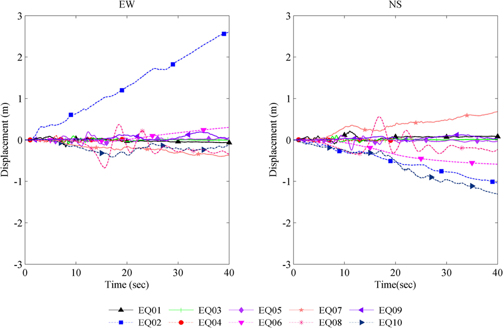
Figure 9. Ground motion displacement time series using Newmark’s integration.

The seismic responses of the vehicles for the selected earthquakes were calculated for various conditions; we assumed that when a vehicle is moving at a speed of more than 5.0 m/s, there will be the driving force with constant acceleration to keep on driving that will nullify the rolling resistance. Hence, the effect of the rolling resistance will be significant only when the vehicle is moving at speeds below 5.0 m/s. We modeled the three vehicle types (i.e., car, bus, and truck) in each of the analysis cases. Figure 10 shows the response of the vehicles at rest in the longitudinal direction (top panels) and in the lateral direction (lower panels). The first, second, and third columns show the response of the car, bus, and truck, respectively. The bus has the largest response even though the mass of the truck is larger than that of the bus, potentially because the maximum turning angle of front tire plays a role.

FIGURE 10

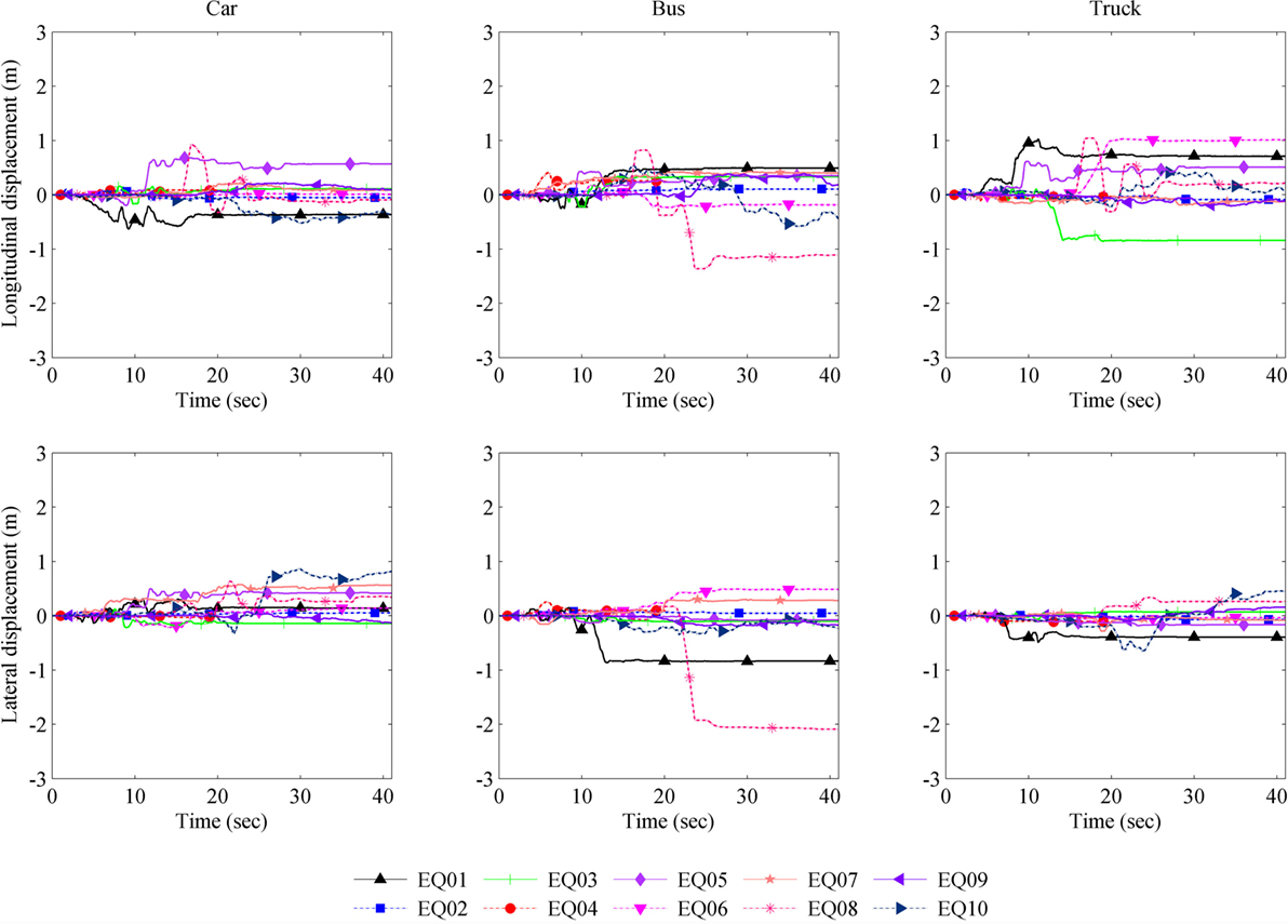
Figure 10. Longitudinal and lateral responses of three vehicles (car, bus, and truck) at rest to acceleration ground motion of ten earthquakes.

We assumed an ideal scenario of a vehicle moving at a certain speed where the driver does not react to the effects of the earthquake and the vehicle is moving freely at a constant speed. The responses of the moving vehicles with a constant speed of 20.0 m/s are shown in Figure 11. The longitudinal displacements are the seismic displacements of the vehicle, where the displacement due to the initial constant speed of the vehicle is unknown. It is worth noting that the longitudinal response of the El Centro earthquake (CA, USA) deviates from the general trend of the other earthquakes, which may be attributed to the effect of the residual acceleration (Figure 9). The accumulated acceleration in the longitudinal direction sustains a higher momentum on the vehicle, pushing it further in the longitudinal direction. The lateral responses of the vehicles vary for the different cases mainly because of deviations in the moving trajectory of the vehicle.

FIGURE 11

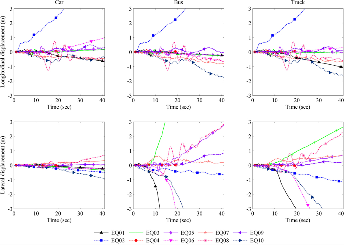
Figure 11. Longitudinal and lateral responses of three vehicles (car, bus, and truck) moving at a constant speed of 20.0 m/s to acceleration ground motion of ten earthquakes.

In many cases, the deviation of a vehicle’s path due to ground motion effects leads to unreal values for the maximum response. Therefore, we fixed the time window to check the maximum response. We selected a time window for tracing of the maximum response as the time of PGA plus an extra 5 s for each case. The maximum response of the vehicle in the given time frame is then identified. Table 5 shows the time of PGA and the corresponding time window used for each earthquake.

TABLE 5

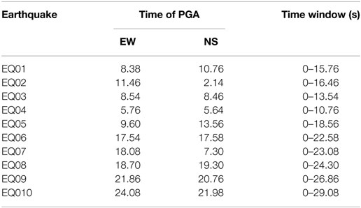
Table 5. Time of PGA occurrence and the time window selected for picking the maximum vehicle response.

We performed the simulation for the 10 selected earthquake records with different vehicle speeds; the modeled PGA remains the same as that which was recorded during those events. The relationship between the maximum longitudinal and lateral responses of the vehicles and the velocity are shown in Figure 12. The maximum response of the vehicles occurred at speeds of about 2.0 m/s; the response then decreased gradually as the velocity increased to about 10.0 m/s and then slightly increased. The car showed the smallest displacements whereas the truck and bus were more affected by misalignment. There were sudden changes in the maximum response over a range of velocities up to 5 m/s, which are mainly due to the use of linear equations in this method. The linear momentum of a vehicle moving at a lower velocity is less than that of a vehicle with a higher velocity; at the same time, the force exerted due to earthquake shaking remains unchanged as replicated in Figure 12.

FIGURE 12

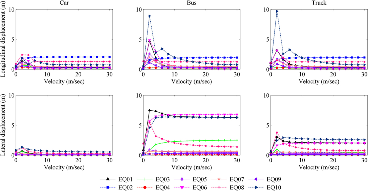
Figure 12. Changes in the maximum longitudinal and lateral responses of the three vehicle types with increasing velocity.

Figure 13 shows the changes in the maximum longitudinal and lateral displacements with PGA of 1–15 m/s² and at a constant vehicle speed of 20.0 m/s. The earthquake ground motions were scaled to the same magnitude before the analysis.

FIGURE 13

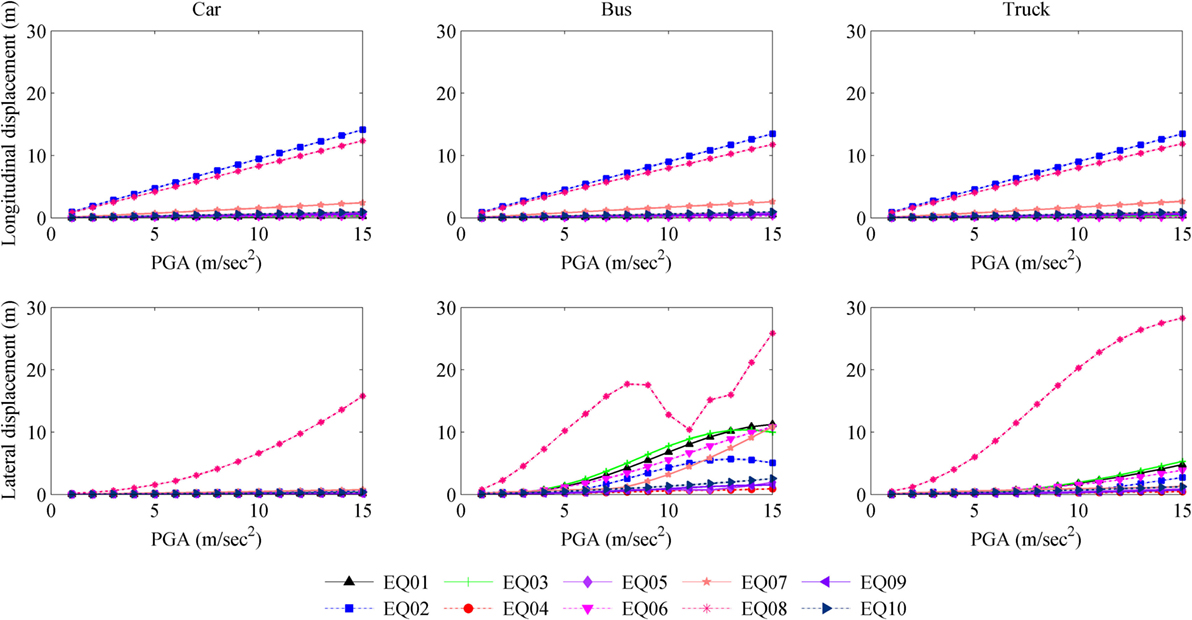
Figure 13. Changes in the maximum longitudinal and lateral responses of vehicles with increasing PGA at constant vehicle speed of 20.0 m/s.

The longitudinal response of the vehicle plays a vital role in the vehicle control during the earthquake and may lead to a collision, depending on the vehicle speed. The responses of the vehicles during the simulated earthquakes varied. The longitudinal response of each vehicle increased linearly as the velocity increased for speeds higher than 10.0 m/s. The results also show that vehicles moving at just 2.0 m/s are at higher risk of losing control. As the velocity of the vehicle increases from a resting state, the vehicle response increases as the vehicle gains speed up to 2.0 m/s and then the response trends downward as the speed rises to 10.0 m/s. The effect of rolling resistance is felt at speeds up to 5.0 m/s and the response fluctuates in this range. The CPLM method takes into account the momentum of the vehicle, which is linearly dependent on the velocity of the vehicle. Hence, the longitudinal responses change linearly with the velocity for speeds higher than 10.0 m/s.

The lateral response of the vehicle is another risk factor. Lateral movement may result in vehicles moving into another lane or onto the shoulder of the road, causing an accident. The lateral movement of the bus was found to be higher than that of the truck or car for similar cases. When the vehicle velocity increases, the lateral response curve is similar to the longitudinal response curve. The maximum turning angle is another major factor in calculating the response; the bus has a maximum turning angle of 38.7° whereas the car and truck have turning angles of 31.7° and 31.6°, respectively.

When the PGA data of all the earthquakes are scaled to the same values, the longitudinal responses of the vehicles seem to vary linearly relative to the ground motion, whereas the lateral responses do not follow the trend seen in the cases of velocity changes for real earthquakes. The ground motion characteristics of the earthquakes have a strong effect on the vehicle response. For example, the Gorkha earthquake resulted in the strongest response with much diversity of motion in both longitudinal and lateral directions. The El Centro earthquake also resulted in a strong longitudinal response, similar to that of the Gorkha earthquake for all vehicle cases.

Vehicle response during the earthquake shaking also depends on the direction in which the vehicle is moving with respect to the components of earthquake acceleration. The left side of Figure 14 shows a polar plot of the maximum longitudinal (X) and lateral (Y) responses for the car example during the Gorkha earthquake within a given time window. The right side of the same figure shows a plot of the longitudinal (X) and lateral (Y) components of the Gorkha earthquake acceleration in a 24.3 s time window with a sampling frequency of 50 Hz. The longitudinal response is more varied than the lateral response in the case of Gorkha earthquake. The shape of the loop of the maximum longitudinal response compares closely with the outer envelop of the acceleration plot. The initial orientation of the vehicle (150°), or its opposite with the longitudinal axis, will be at highest risk whereas the lowest risk associated with the vehicle will be when it is oriented perpendicular to those angles.

FIGURE 14

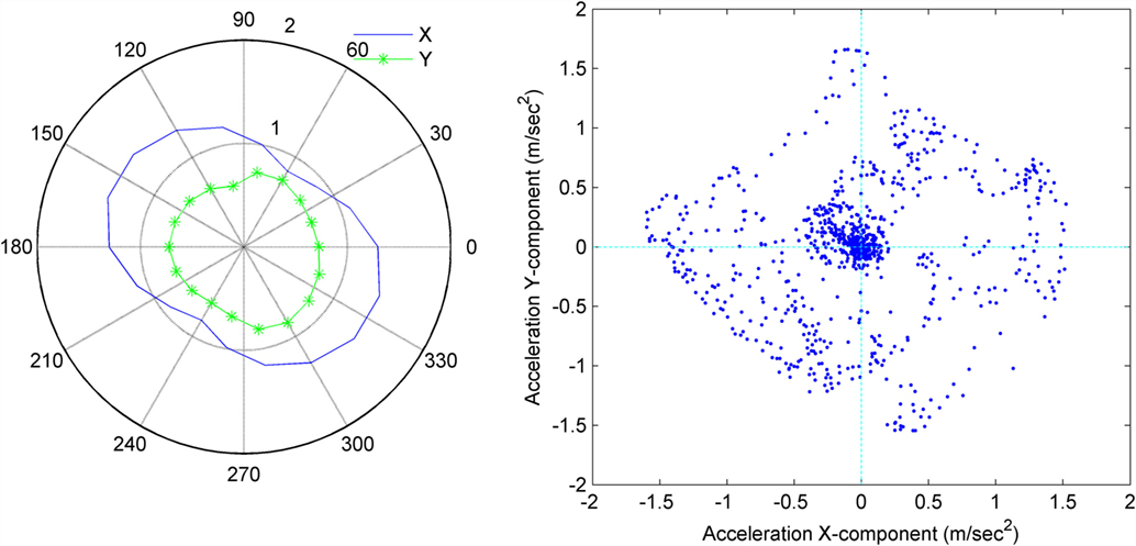
Figure 14. Variation of the maximum longitudinal (X) and lateral (Y) response of the vehicle with different orientation of the vehicle (left) and plot X-component and Y-component of acceleration vector of Gorkha earthquake for time window of 24.30 s (right).

Conclusion

In this study, we have proposed a model that simulates vehicle responses to the maximum ground acceleration of earthquakes within a fixed time window for each event, assuming ideal vehicle conditions. Analysis of video footage of vehicle motion during the Gorkha earthquake supported the results of the simulation undertaken with the CPLM method. The CPLM method can be used effectively in scenarios with a range of vehicle speeds, including being at a full stop. In a real earthquake scenario, vehicle conditions will be different from the ideal situation, and the driver’s behavior will be a major factor. We have discussed the maximum response of the vehicles within the fixed time window; however, this requires further research. The time it takes for the driver to recognize that an earthquake is occurring is important for simulating the driver’s behavior and actions in the model. Additionally, issues concerning the provision of information to drivers about the earthquake – e.g., an early warning system that may enable drivers to react and prevent accidents – should be investigated further. Unlike the smooth driving conditions used in the simulation, moving vehicles in reality will shake as a result of irregular road conditions or mechanical issues, making it difficult for drivers to identify shaking caused by ground motion.

Our results show that the response of the vehicles depends mainly on the ground motion characteristics and orientation of the vehicle, rather than on the PGA excitation alone. Slow moving vehicles have a higher risk of being affected than faster ones; hence, vehicles in the city are more at risk. However, slow vehicles are easier to control than faster ones; therefore, vehicle drivers in an urban setting have better steering control and are able to react more quickly. Thus, their level of risk is lower compared with vehicles in an ideal situation (i.e., with no driver reaction).

The authors are working further on research to incorporate the driver’s reaction and response during earthquake shaking. The CPLM method will be used for the response mechanisms of various vehicle models whereas the driver’s control over the steering system while following other vehicles will be analyzed using a driving simulator experiment.

Author Contributions

All authors listed, have made substantial, direct and intellectual contribution to the work, and approved it for publication.

Conflict of Interest Statement

The authors declare that the research was conducted in the absence of any commercial or financial relationships that could be construed as a potential conflict of interest.

Supplementary Material

The Supplementary Material for this article can be found online at https://www.frontiersin.org/article/10.3389/fbuil.2016.00016

References

AASTHO. (2001). A Policy on Geometric Design of Highways and Streets. Washington: American Association of Highway and Transportation Association.

Google Scholar

Alagappan, A. V., Rao, K. V. N., and Kumar, R. K. (2014). A comparison of various algorithms to extract Magic Formula tyre model coefficients for vehicle dynamics simulations. Veh. Syst. Dyn. 53, 154–178. doi: 10.1080/00423114.2014.984727

CrossRef Full Text | Google Scholar

Guiggiani, M. (2014). The Science of Vehicle Dynamics: Handling, Braking, and Ride of Road and Race Cars. Netherlands: Springer.

Google Scholar

JMA. (1996). The Japan Metereological Agency (JMA) Seismic Intensity Scale. Available at: http://www.jma.go.jp/jma/kishou/know/shindo/index.html (in Japanese)

Google Scholar

Kawashima, K., Sugita, H., and Kanoh, T. (1989). Effect of earthquake on driving of vehicle based on questionnaire survey. Struct. Eng. Earthq. Eng. 6, 405–412.

Google Scholar

Li, L., Yang, K., Jia, G., Ran, X., Song, J., and Han, Z. Q. (2015). Comprehensive tire-road friction coefficient estimation based on signal fusion method under complex maneuvering operations. Mech. Syst. Signal Process. 56, 259–276. doi:10.1016/j.ymssp.2014.10.006

CrossRef Full Text | Google Scholar

Maruyama, Y., and Yamazaki, F. (2002). Seismic response analysis on the stability of running vehicles. Earthq. Eng. Struct. Dyn. 31, 1915–1932. doi:10.1002/eqe.195

CrossRef Full Text | Google Scholar

Maruyama, Y., and Yamazaki, F. (2006). Relationship between seismic intensity and drivers’ reaction in the 2003 Miyagiken-Oki earthquake. Struct. Eng. Earthq. Eng. 23, 69s–74s. doi:10.2208/jsceseee.23.69s

CrossRef Full Text | Google Scholar

NIED. (2015). Strong-motion Seismograph Networks (K-NET, KiK-net). Available at: http://www.kyoshin.bosai.go.jp/

Google Scholar

Pacejka, H. B. (2006). Tyre and vehicle dynamics. Mater. Mech. 172–190. doi:10.1016/B978-075066918-4/50011-3

CrossRef Full Text | Google Scholar

Parajuli, R. R., and Kiyono, J. (2015). Ground motion characteristics of the 2015 gorkha earthquake, survey of damage to stone masonry structures and structural field tests. Front. Built Environ. 1:23. doi:10.3389/fbuil.2015.00023

CrossRef Full Text | Google Scholar

Toyota. (2015). Toyota HiAce Specifications. Available at: http://www.toyota.com.au/static/vehicles/hiace/content/pdf/hiace_saver.pdf?

Google Scholar

USGS. (2015). Center for Engineering Strong Motion Data. Available at: http://strongmotioncenter.org/

Google Scholar

Wong, J. Y. (2001). Theory of Ground Vehicles, Third Edn, Vol. 1. John Wiley & Sons, Inc.

Google Scholar