Multihazard Hurricane Fragility Model for Wood Structure Homes Considering Hazard Parameters and Building Attributes Interaction

Introduction

Data-based fragility models account for a range of variables (Nateghi et al., 2011; Pitilakis et al., 2014), model damage as a function of multiple hazard parameters and building attributes, consider variability in building and environmental attributes, and use field data to predict future damage and validate model performance. If field data are representative of a range of hazard parameters, building attributes, and building damage data, data-based models will effectively predict damage, and identify variables that significantly contribute to damage. In addition to their simplicity, data-based models are more realistic than simulation-based models, as the models are developed based on observed data. On the other hand, the availability of data and presence of missing data due to severity of damage may be a common issue for these models. Another issue is subjectivity of the model results particularly, when damage is assessed without a defined damage scale. Data-based fragility models have been widely implemented to estimate the probability of collapse or being in or exceeding a specified damage state for buildings subjected to tsunami (e.g., Reese et al., 2007, 2011; Koshimura et al., 2009; Suppasri et al., 2012, 2013; Charvet et al., 2014a,b, 2015; Muhari et al., 2015) and earthquake (Porter et al., 2007; Tang et al., 2012; Lallemant et al., 2015). Although not specific to building, Padgett et al. (2012) empirically modeled damage to coastal bridges along the US Gulf Coast using multivariate logistic regression models, Reed et al. (2016) developed a logit fragility model to predict damage for power systems, and Kameshwar and Padgett (2018) developed a wind buckling and storm surge flotation fragility models for oil storage tanks.

Specific to coastal building subjected to hurricane hazards, data-based fragility models have been used to estimate building damage as a function of hazard parameters (H), environmental (E), and building attributes (A). Tomiczek et al. (2014a) developed a multivariate regression fragility model for pile-elevated wood structures to estimate the probability of collapse as a function of H (i.e., maximum current velocity, breaking wave height, maximum significant wave height) and A (i.e., freeboard height, building age). Massarra et al. (2019) developed a predictive data-based fragility models to predict the probabilities of a home being in or exceeding a certain damage state and complete failure as a function of H (i.e., maximum significant wave height, maximum 3-s gust wind speed, and maximum water speed). Specific to coastal building subjected to storm surge, Hatzikyriakou et al. (2015) developed a logistic regression fragility model for single-family home component to predict the probability of collapse as a function of E (i.e., distance from the coast, ground elevation,) and A (i.e., elevation of the lowest horizontal member, structure height above lowest horizontal member, house age, building perimeter), and Hatzikyriakou and Lin (2018) developed a cumulative logit fragility model to predict the probability of a home being in or exceeding a certain damage state as a function of H (i.e., flood inundation, wave height, dune erosion) and E (i.e., base flood elevation) with the exclusion of building attributes (A). In the previous studies, building damage was modeled as a function of main explanatory variable effects (i.e., H, E, A), where none of these studies modeled damage as a function of H, E, A, and their interactions (e.g., HE, HA, EA). Interaction terms are variables that result from the product of two (i.e., two-factor interaction terms) or more main explanatory variables.

For example, a model with explanatory variables (H) and (A), where H represents surge depth and A represents foundation type (e.g., slab and elevated), is defined as a model with main explanatory variables. While modeling building damage as a function of main explanatory variables reflects the simultaneous effect of these variables on damage, failure to account for the interactions lead to bias and misinterpretation of the model coefficients. Significant interaction terms reflect variation in the effect of one main explanatory variable on the response variable based on levels of another main explanatory variables (Jaccard and Turrisi, 2003). Therefore, to understand the variation in the effect of increased surge depth on damage for building built on slab and those elevated, the two-factor interaction (HA) between surge and foundation is modeled and interpreted.

Interaction between H and A has been less frequently considered and modeled. Tomiczek et al. (2017) used multiple linear regression models to estimate probability of building damage as a function of H (i.e., maximum water depth, maximum water velocity), A (i.e., relative shielding, age minimum freeboard), and HA interaction (i.e., maximum water velocity and relative shielding). They found that HA interaction term is an important factor that significantly contributes to damage; however, the interpretation of the coefficients was limited to just the indication of the degree of significance, which does not reflect variation in the effect of maximum water velocity on probability of damage based on levels of relative shielding. When considering H, E, and A in the fragility models, two-factor interaction terms between continuous and categorical variables (i.e., HA, EH) are easier and more meaningful to interpret than two-factor interaction terms between continuous variables (i.e., HH, EE) or between categorical variables (i.e., AA). In the current literature, HA interaction terms have not been directly modeled and interpreted in the development of data-based building fragility model. When HA terms are statistically significant, they indicate that the effect of H on damage varies for the levels of A; therefore, damage must be predicted based on both main and interaction terms.

This paper develops data-based fragility models for wood structure homes as a function of continuous variables (H, E), categorical variables (A), and the two-factor interaction (HA) of H and A variables. The H variables are maximum 3-s gust wind speed, maximum significant wave depth, maximum surge depth, and maximum water speed. The E variable is the Federal Emergency Management Agency (FEMA)-derived base flood elevation. The A variables are foundation type and number of stories. The HA interactions are the product of H and A variables, resulting in eight interaction terms. Videographic global damage data and building attributes recorded in coastal Mississippi, simulated hazard data computed by the Simulating WAves Nearshore and ADvanced CIRCulation (SWAN+ADCIRC) model, and base flood elevation values derived from Flood Insurance Rate maps (FIRMs) are the model inputs. Historical FIRM_S for Hancock (1983, 1987, 1992), Harrison, (1980, 1983, 1984, 1988, 2002), and Jackson (1983, 1987, 1992) Counties (Mississippi), respectively, were used to obtain base flood elevation. The historic FIRM_S were downloaded from FEMA. Each portion of every county in the study area had a specific historic FIRM. As a result, multiple historical FIRMs were available for every county and not for every building in the study area. The year of the FIRMs includes multiple FIRMs for each county in the study area and not for a specific building. The flood maps are georeferenced in Geographic Information System (ArcGIS), and base flood elevation values are recorded at building footprint locations. Overall building damage (i.e., global building damage) is assessed using the Wind and Flood (WF) Damage Scale developed by Friedland and Levitan (2009). Proportional odds cumulative logit and logistic regression models are used to estimate the probability of being in or exceeding a specified DS and the probability of collapse, respectively. Model prediction accuracy is evaluated using “leave-one-out” cross-validation (LOOCV) and expressed in terms of the cross-classification rate (CCR).

Data

Global Building Damage State and Building Attributes Variables

High-definition, geo-referenced videos were collected for residential buildings using the VIEWS^TM system (Adams et al., 2004) in Hancock, Harrison, and Jackson Counties of coastal Mississippi (Figure 1). Videographic data collection has been proven to be a valid and effective approach for rapid damage assessment in many post-disaster studies (Curtis et al., 2007a,b, 2010). It was also found that videographic approach has several key benefits over field surveys, including reduced cost, creation of a digital record, and the ability to process the images quickly (Lue et al., 2014). The field deployment took place on September 6–11, 2005 after Hurricane Katrina as part of the Multidisciplinary Center for Earthquake Engineering Research (MCEER) reconnaissance. The high-definition, geo-referenced video camera was mounted on the passenger side of a slowly moving vehicle, and data were recorded. After the reconnaissance was completed, the videos and still images extracted from these videos were reviewed to document building attributes and global building damage for every building along the driving route by surveying the parts of the buildings captured on the videos (e.g., front and side of the building). For each surveyed building, the overall observed building damage (e.g., minor damage, moderate damage, severe damage) was visually assessed using the Wind and Flood (WF) Damage Scale developed by Friedland and Levitan (2009). Building attributes (e.g., foundation type, number of stories) were also visually documented for each surveyed building. Roof damage was assessed using 0.3 m spatial resolution post-event National Oceanic and Atmospheric Administration (NOAA) aerial color images. The database source for the land parcel is Mississippi Automated Resource Information System (MARIS). Building footprint polygons are from the City of Biloxi, City of Gulfport, Southern Mississippi Planning and Development District, and Jackson County.

FIGURE 1

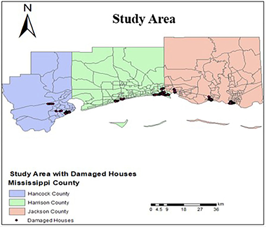
Figure 1. Study areas and building observation locations.

The WF Damage Scale categorizes global combined wind and flood residential building damage into seven damage classes ranked WF0 through WF6. The WF Damage Scale has been previously adopted by Massarra et al. (2019) and modified and applied by Hatzikyriakou (2017), Tomiczek et al. (2017), and Zhang et al. (2017) to classify building damage data obtained from field reconnaissance. A database that includes land parcel data and building footprint polygons was developed using a geographic information systems (ArcGIS). The building location in the study area was represented using the calculated centroid for each building footprint. The building in the study area were wood-framed, one- and two-story residential homes built on slabs or elevated foundations and with siding or brick cladding. Few buildings with characteristics differing from the previous characteristics were found in the study area. These buildings along with those with unassessed damage states were excluded from the analysis, resulting in a final dataset of 866 single-family homes (Table 1) that describes the global building damage sates (DS), number and percentage of buildings, slabs, elevated foundation, and one and two stories in each damage level. For the uncertainties associated with damage assessment and to ensure that damage levels recorded by one assessor match those that would be recorded by another assessor, buildings in the study area were assessed by two assessors. A confusion matrix showing assessment results was then developed (Massarra et al., 2019), where a cross-classification rate (CCR) of 99% was found between the two assessors.

TABLE 1

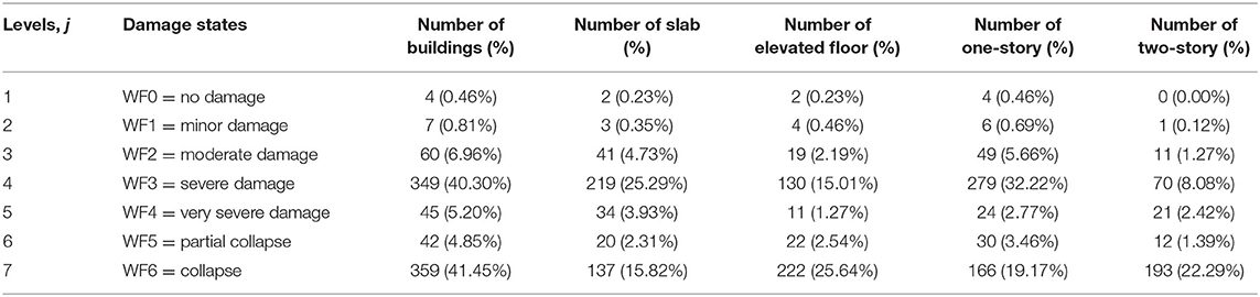
Table 1. Frequency and percentage % of global building damage states, foundation type, and number of stories.

A low number of observations in WF0, WF1, WF4, and WF5 was found, which may indicate issues in model fitting. Lillesand et al. (2014) recommended that a minimum of 50 observations be collected for each DS level; therefore, WF DS were grouped to represent the DS response variable Y. Grouped WF DS with low number of observations are considered less reasonable models for damage prediction and were excluded from consideration resulting in DS response variable Y for n models, each with j levels, DS_j,n (Table 2). Models 1–9 represent models with ordered multinomial categorical response variables, while models 10 and 11 represent models with binary response variables.

TABLE 2

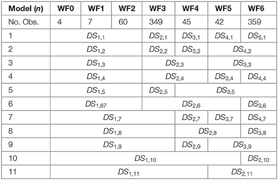
Table 2. Model (n), number of observations in each Wind and Flood (WF) damage states (DS), and global building DS response variable levels for each model, DS_j,n.

Simulated Explanatory Hazard Variables

Hazard parameters are characterized by wind speeds, significant wave heights, and water levels during Katrina at the building sites. Because these variables were not observed during the storm at all locations, it is necessary to use a high-resolution, predictive modeling system to represent their spatial and temporal variations during the storm. The tightly coupled ADvanced CIRCulation (ADCIRC) and Simulating WAves Nearshore (SWAN) models have been well-validated for Katrina simulations, with a mean absolute error within 0.25 m (Dietrich et al., 2010).

It can be challenging to predict the evolution of individual waves over a large geographical domain, and thus, it is common for wave models to predict the evolution of wave energy, which can then be integrated to determine variables like the significant wave height, mean wave period, etc. SWAN solves the spectral action balance equation for the action density N(t, λ, φ, σ, θ), which can vary in time t, geographic space (λ, φ) with longitudes λ and latitudes φ, and spectral space (σ, θ) with frequencies σ and directions θ (Booij et al., 1999). SWAN was extended in its functionality (Zijlema, 2010) and then coupled tightly with ADCIRC, which solves modified forms of the shallow water equations for the evolution of the total water depth H = h + ζ, where h is the local bathymetry and ζ is the free surface elevation relative to the geoid, and the depth-averaged current velocities U and V (Luettich and Westerink, 2004; Westerink et al., 2008).

ADCIRC passes the local water depths and current velocities, which are used by SWAN to compute the changes in wave energy due to refraction and frequency shifting. SWAN passes the local radiation stress gradients, which are used by ADCIRC as surface stresses in its momentum equations. Storm-driven waves and surge can evolve over a wide range of spatial scales, with a grid size from kilometers in deep water and on the continental shelf, to tens of meters in small manmade and natural channels in coastal regions. SWAN+ADCIRC describes these spatial scales by using an unstructured mesh with triangular, finite elements, which can vary in size so that resolution (and thus accuracy) can be increased in regions of specific interest. The model results in this study were computed on the SL16 mesh, which was developed and validated for the devastating Gulf hurricanes of 2005 and 2008 (Dietrich et al., 2012a,b). This mesh provides high-resolution coverage of the northern Gulf coast from western Louisiana through Alabama, including where building damage states were observed along the Mississippi coast. In these regions, the mesh resolution is typically about 100 m in coastal floodplains, with higher resolution in channels and near hydraulic features. This resolution does not allow for predictions of smaller-scale processes like wave set-up and interaction with built infrastructure, but it does allow for wide coverage of storm hazards along the entire region affected by Katrina.

The wave and surge models are forced by wind fields that were developed using objectively analyzed, airborne, and land-based measurements. The measurements are assimilated into the Hurricane Research Division Wind Analysis System (H^*WIND; Powell et al., 2010) and then blended with Gulf-scale winds using an Interactive Objective Kinematic Analysis (IOKA; Cardone et al., 2007). The winds represent 10-min sustained wind speeds at 10 m elevation and are then interpolated onto a regular 0.05 × 0.05 grid with snapshots every 15 min, which are read and applied in SWAN+ADCIRC. For the estimation of building damages, these winds were converted to an averaging period of 3 s (Krayer and Marshall). Thus, for the data-based fragility analyses, the model outputs were interpolated at the building locations to provide time series of wind speed (U₁₀; m/s), significant wave height (H_S; m), water level (ζ; m relative to NAVD88), and water speed (U and V; m/s). U₁₀ is provided at an elevation of 10 m and converted to an averaging period of 3 s; H_S is computed by integrating the action density in spectral space in SWAN; ζ is computed by ADCIRC and is representing the combined contributions of tides, storm surge, and wave-induced setup; and U is computed by ADCIRC and represents the depth-averaged velocities at each location.

For the uncertainties associated with hazard parameters, observations for peak wind speeds at 11 buoys, peak wave heights at 17 stations, and peak water levels at 354 stations were used during Hurricane Katrina (2005). To the authors' knowledge, peak current speeds were observed at seven stations along the Mississippi and Alabama coasts during the Deepwater Horizon oil spill (2010) but not during Hurricane Katrina or other recent storms in this region. SWAN+ADCIRC was previously validated using the same observations (Dietrich et al., 2012a,b). These observations were used to quantify the prediction uncertainties by calculating mean absolute errors and standard deviations at these stations. Mean absolute error was found to be 2.83 m/s, 1.07 m, 0.20 m, and 0.67 m/s for peak wind speeds, peak wave heights, peak water levels, and peak current speeds, respectively. Standard deviation was found to be 2.84 m/s, 1.44 m, 0.3 m, 0.26 m/s for peak wind speeds, peak wave heights, peak water levels, and peak current speeds, respectively. With such a large and complex domain, the calculated error statistics indicate a high level of accuracy as well as the uncertainties associated with hazard parameters.

Table 3 lists the continuous explanatory variables (X_h) and (X_BFE) and the binary categorical variables (Z_a) used to fit the fragility models. Variable X_h are the maximum values of the time series obtained from the coupled SWAN+ADCIRC models. The maximum surge depth (D_max) at the centroid of each building footprint was calculated as the difference between maximum water level (ζ_max) and the bathymetry/topography (m) of the SL16 mesh (NAVD88) at that location. The maximum surge depth within the building (D_W,max) was calculated as the difference between surge depth (D_max) and h, where h is the approximate first floor elevation of each house in meters. Approximate first floor elevation was calculated as the sum of the top of the lowest floor height above the local ground and topography at that location, where the top of the lowest floor height above the local ground was estimated by counting the number of building steps and assuming an average 17.8 cm (7 in) step rise. The maximum significant wave depth (H_d,max) was calculated as (H_S,max + D_max) – h. Variable Z_a is the building attribute that represents binary foundation (Z_FT) and number of stories(Z_NS), where the two levels are defined as slab (Z_{FT, 0}), elevated (Z_{FT, 1}), one story (Z_{NS, 0}), and two stories (Z_{NS, 1}). Multicollinearity among continuous variables was evaluated using the variance inflation factor (VIF). Positive correlation was found for maximum significant wave height and maximum surge depth; therefore, H_S,max and D_max were not included in the same fragility model.

TABLE 3

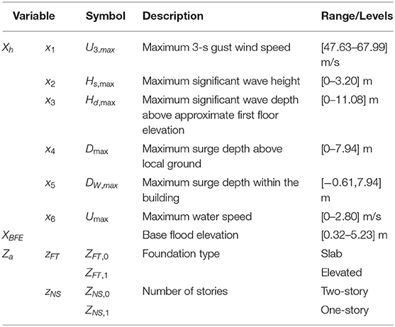
Table 3. Explanatory variables used to construct the fragility models.

Methodology

Fragility Modeling

Generally, one-dichotomy (e.g., collapse or no collapse) response variable is evaluated using binary logistic regression models. For response variable Y with two levels (models 10 and 11) and H hazard variables x₁, x₂, …, x_H, one E environmental X_BFE variable, and A building attribute variables z₁, z₂, …, z_A (Table 3), the generalized forms of binary logistic regression, without and with HA interaction terms, respectively, are given as

$\begin{array}{l}\text{logit}[P]=ln\left[\frac{P}{1-P}\right]=\alpha +{\displaystyle \sum _{h=1}^H}{{\beta }_{h}x}_h+{\beta }_b{X}_{BFE}\\ +{\displaystyle \sum _{a=1}^A}{{\gamma }_{a}z}_a,\text{and }& (1)\end{array}$

$\begin{array}{l}\text{logit}[P]=ln\left[\frac{P}{1-P}\right]=\alpha +{\displaystyle \sum _{h=1}^H}{{\beta }_{h}x}_h+{\beta }_b{X}_{BFE}+{\displaystyle \sum _{a=1}^A}{{\gamma }_{a}z}_a\\ +{\displaystyle \sum _{h=1}^H}{\displaystyle \sum _{a=1}^A}{\eta }_{ha}{x}_h{z}_a,& (2)\end{array}$

where P denotes the probability of collapse; logit[P] is the logit link function, which is equal to the natural logarithm (log) of the odds of collapse; α is the model intercept; β_h are hazard coefficients, β_b is base flood elevation coefficient, γ_a are building attribute coefficients, and η_ha are hazard and building attribute interaction term coefficients.

Based on Equations (1) and (2), respectively, the estimated probability of collapse is calculated as

$\begin{array}{ll}P=\frac{exp\left(\alpha +{\displaystyle {\sum }_{h=1}^H}{{\beta }_{h}x}_h+{\beta }_b{X}_{BFE}+{\displaystyle {\sum }_{a=1}^A}{{\gamma }_{a}z}_a\right)}{1+exp\left(\alpha +{\displaystyle {\sum }_{h=1}^H}{{\beta }_{h}x}_h+{\beta }_b{X}_{BFE}+{\displaystyle {\sum }_{a=1}^A}{{\gamma }_{a}z}_a\right)},& (3)\end{array}$

$\begin{array}{ll}P=\frac{exp\left(\alpha +{\displaystyle {\sum }_{h=1}^H}{{\beta }_{h}x}_h+{\beta }_b{X}_{BFE}+{\displaystyle {\sum }_{a=1}^A}{{\gamma }_{a}z}_a+{\displaystyle {\sum }_{h=1}^H}{\displaystyle {\sum }_{a=1}^A}{\eta }_{ha}{x}_h{z}_a\right)}{1+exp\left(\alpha +{\displaystyle {\sum }_{h=1}^H}{{\beta }_{h}x}_h+{\beta }_b{X}_{BFE}+{\displaystyle {\sum }_{a=1}^A}{{\gamma }_{a}z}_a+{\displaystyle {\sum }_{h=1}^H}{\displaystyle {\sum }_{a=1}^A}{\eta }_{ha}{x}_h{z}_a\right)},& (4)\end{array}$

For response variable Y with ordered categorical multinomial response variables (models 1–9), logistic regression is extended to the proportional odds cumulative logit model, which uses cumulative probabilities to evaluate ordered categories with the assumption that curves of the various cumulative logits are parallel. The odds show how likely it is to move up by one level in the ordinal outcome (e.g., odds of being in DS₃ rather than DS₂, or odds of being in DS₂ rather than DS₁). There is a primary assumption of proportional odds regression (i.e., proportional odds assumption). The odds must be the same across each level of the ordinal outcome for the effect to be valid. With this said, the odds of inclusion are the same for all categories. The log odds of response variable Y being in level j or greater, without and with HA interactions, respectively, are given for j ≥ 2 as

$\begin{array}{l}\text{logit}\left[P(Y\ge j)\right]=ln\left[\frac{P(Y\ge j)}{1-P(Y\ge j)}\right]={\alpha }_j+{\displaystyle \sum _{h=1}^H}{{\beta }_{h}x}_h\\ +{\beta }_b{X}_{BFE}+{\displaystyle \sum _{a=1}^A}{{\gamma }_{a}z}_a,\text{and}& (5)\end{array}$

$\begin{array}{l}\text{logit}\left[P(Y\ge j)\right]=ln\left[\frac{P(Y\ge j)}{1-P(Y\ge j)}\right]={\alpha }_j+{\displaystyle \sum _{h=1}^H}{{\beta }_{h}x}_h\\ +{\beta }_b{X}_{BFE}+{\displaystyle \sum _{a=1}^A}{{\gamma }_{a}z}_a+{\displaystyle \sum _{h=1}^H}{\displaystyle \sum _{a=1}^A}{\eta }_{ha}{x}_h{z}_a,& (6)\end{array}$

where the interactions between building attributes and hazard are represented as the sum of hazard and building attribute product terms “x_hz_a.” Both Equations (5) and (6) result in a set of J – 1 equations with unique intercepts (α_j) and common slopes (β_h, β_b, γ_a, η_ha).

Based on Equations (5) and (6), the estimated probability of Y being in or exceeding level j is calculated for j ≥ 2 as

$\begin{array}{ll}P(Y\ge j)=\frac{exp\left({\alpha }_j+{\displaystyle {\sum }_{h=1}^H}{{\beta }_{h}x}_h+{\beta }_b{X}_{BFE}+{\displaystyle {\sum }_{a=1}^A}{{\gamma }_{a}z}_a\right)}{1+exp\left({\alpha }_j+{\displaystyle {\sum }_{h=1}^H}{{\beta }_{h}x}_h+{\beta }_b{X}_{BFE}+{\displaystyle {\sum }_{a=1}^A}{{\gamma }_{a}z}_a\right)}\text{for }j=2\dots J.& (7)\end{array}$

$\begin{array}{ll}P(Y\ge j)=\frac{exp\left({\alpha }_j+{\displaystyle {\sum }_{h=1}^H}{{\beta }_{h}x}_h+{\beta }_b{X}_{BFE}+{\displaystyle {\sum }_{a=1}^A}{{\gamma }_{a}z}_a+{\displaystyle {\sum }_{h=1}^H}{\displaystyle {\sum }_{a=1}^A}{\eta }_{ha}{x}_h{z}_a\right)}{1+exp\left({\alpha }_j+{\displaystyle {\sum }_{h=1}^H}{{\beta }_{h}x}_h+{\beta }_b{X}_{BFE}+{\displaystyle {\sum }_{a=1}^A}{{\gamma }_{a}z}_a+{\displaystyle {\sum }_{h=1}^H}{\displaystyle {\sum }_{a=1}^A}{\eta }_{ha}{x}_h{z}_a\right)}\text{for }j=2\dots J.& (8)\end{array}$

For the first level (j = 1), the estimated probability of Y being in or exceeding this damage level is equal to 1. The estimated probability that the DS falls into a specific categorical damage level [i.e., P(Y = j)] is calculated for levels j ≤ J – 1 as

$\begin{array}{ll}P\left(Y=j\right)=P\left(Y\ge j\right)-P\left(Y\ge j+1\right)\text{ for }j\le J-1.& (9)\end{array}$

To interpret the influence of increasing continuous main effects (i.e., X_h, X_BFE) on damage, the specific odds ratios (MOR_h) and (MOR_BFE) for two values of x_h (i.e.,x_h1, x_h2) and X_BFE (i.e., x_BFE1, x_BFE2) with M_h unit increase, where M_h = x_h2 − x_h1, and M_BFE unit increase, where _{MBFE = xBFE2} − x_BFE1, respectively, are calculated as

$\begin{array}{ll}{\text{MOR}}_{h(1,2)}=\exp \left[M_h{\beta }_h)\right]=\frac{\frac{P\left(Y\ge j|X_h=x_{h1}\right)}{P\left(Y<j|X_h=x_{h1}\right)}}{\frac{P\left(Y\ge j|X_h=x_{h2}\right)}{P\left(Y<j|X_h=x_{h2}\right)}},\text{and}& (10)\end{array}$

$\begin{array}{ll}{\text{MOR}}_{BFE(1,2)}=exp\left[{M_{BFE}\beta }_b\right]=\frac{\frac{P(Y\ge j|X_{BFE}=x_{BFE1})}{P(Y<j|X_{BFE}=x_{BFE1})}}{\frac{P(Y\ge j|X_{BFE}=x_{BFE2})}{P(Y<j|X_{BFE}=x_{BFE2})}},& (11)\end{array}$

Given that x_h and X_BFE are continuous variables, MOR_{h(1, 2)} and MOR_{BFE(1, 2)} describe the numerical odds of a building being in a higher rather than in a lower damage level for each M_h or M_BFE unit increase in X_h andX_BFE, holding the other variables constant, where M_h and M_BFE are scaling factors that represent multiple or fraction of unit increases in hazard intensities and base flood elevation on the odds ratio. For logistic regression models MOR_{h(1, 2)} and MOR_{BFE(1, 2)} describe the numerical odds of collapse for each M_h or M_BFE unit increase in X_h and X_BFE, holding the other variables constant.

To interpret the influence of the categorical main effect (Z_a), the specific odds ratio (MOR_a) for two levels of z_a (i.e.,z_a0, z_a1) is calculated as

$\begin{array}{ll}{\text{MOR}}_{a(0,1)}=exp({\gamma }_a)=\frac{\frac{P(Y\ge j|Z_a=z_{a1})}{P(Y<j|Z_a=z_{a1})}}{\frac{P(Y\ge j|Z_a=z_{a0})}{P(Y<j|Z_a=z_{a0})}}.& (12)\end{array}$

Given that Z_a is categorical binary variables with levels Z_a0 and Z_a1, MOR_{a(0, 1)} describes the numerical odds of a building being in a higher damage level rather than a lower damage level for Z_a1 compared to Z_a0, holding the other variables constant. For logistic regression models, MOR_{a(0, 1)} describes the numerical odds of collapse for Z_a1 compared to Z_a0, holding the other variables constant.

To interpret the influence of the interaction terms (_XhZa), the odds ratio MOR_{ha(1, 2)} for HA interaction terms is calculated as = exp(M_hη_ha). For proportional odds cumulative logit model, this value describes the numerical odds of a building being in a higher damage level rather than a lower damage level for two values of x_h (i.e., x_h1, x_h2) with M_h unit increase across levels of a building attribute (i.e., Z_{a, 0}, Z_{a, 1}). For logistic regression models, MOR_{ha(1, 2)} describes the numerical odds of collapse for two values of x_h (i.e., x_h1, x_h2) with M_h unit increase across levels of a building attribute (i.e., Z_{a, 0}, Z_{a, 1}). The odds ratio for HA interaction terms also equals the ratio of two odds ratios MOR_{h(1, 2)}|Z_{a, 0} and MOR_{h(1, 2)}|Z_{a, 1} and is given as

$\begin{array}{l}{\text{MOR}}_{ha(1,2)}=\frac{{\text{MOR}}_{h(1,2)}|Z_{a,1}}{{\text{MOR}}_{h(1,2)}|Z_{a,0}}=\frac{exp{M}_h({\beta }_h+{\eta }_{ha})|Z_{a,1}}{exp\left({M_h\beta }_h\right)|Z_{a,0}}\\ =\frac{\frac{P(Y\ge j|X_h=x_{h1})}{P(Y<j|X_h=x_{h1})}|Z_{a,1}}{\frac{P(Y\ge j|X_h=x_{h2})}{P(Y<j|X_h=x_{h2})}|Z_{a,0}},& (13)\end{array}$

For a proportional odds cumulative logit model, MOR_{h(1, 2)}|Z_{a, 0} is the odds of being in a higher rather than in a lower damage level for M_h unit increase in x_h (i.e., x_h1, x_h2) given building attribute level Z_{a, 0}. MOR_{h(1, 2)}|Z_{a, 1} is the odds of being in a higher rather than in lower damage level for M_h unit increase in x_h (i.e., x_h1, x_h2) given building attribute level Z_{a, 1}. For the range of hazard intensity available in this study, the obtained odds are for a specific increase in hazard intensity and vary across different increases in the hazard intensities. The odds show how likely it is to move up on one level in the ordinal outcome (e.g., odds of being in DS₃ rather than DS₂, or odds of being in DS₂ rather than DS₁). There is a primary assumption of proportional odds regression (i.e., proportional odds assumption). The odds must be the same across each level of the ordinal outcome for the effect to be valid. With this said, the odds are the same for all categories.

For logistic regression, MOR_{h(1, 2)}|Z_{a, 0} is the odds of collapse for M_h unit increase in x_h (i.e., x_h1, x_h2) given building attributes level Z_{a, 0}. MOR_{h(1, 2)}|Z_{a, 1} is the odds of collapse for M_h unit increase in x_h (i.e., x_h1, x_h2) given building attribute level Z_{a, 1}.

The 95% lower (LCI) and upper (UCI) confidence intervals for MOR_{h(1, 2)}|Z_{a, 0}, denominator of Equation (13), is given as $exp\left\{M_h\left[{\widehat{\beta }}_h\pm 1.96^{*}SE({\widehat{\beta }}_h)\right]\right\}$, where ${\widehat{\beta }}_h$ are the estimated H coefficients. The 95% lower (LCI) and upper (UCI) confidence intervals for MOR_{h(1, 2)}|Z_{a, 0}, numerator of Equation (13), is given as $\exp \left\{M_h\left[({\widehat{\beta }}_h+{\widehat{\eta }}_{ha})\pm {1.96}^{\ast }SE\left({\widehat{\beta }}_h+{\widehat{\eta }}_{ha}\right)\right]\right\}$, where ${\widehat{\eta }}_{ha}$are the estimated HA coefficients, $SE\left({\widehat{\beta }}_h\right)$ is the standard error of ${\widehat{\beta }}_h$, and $SE\left({\widehat{\beta }}_h+{\widehat{\eta }}_{ha}\right)$ is the standard error of the summation of ${\widehat{\beta }}_h$ and ${\widehat{\eta }}_{ha}$. The standard error $SE\left({\widehat{\beta }}_h+{\widehat{\eta }}_{ha}\right)$is calculated as $\sqrt{var\left({\widehat{\beta }}_h\right)+var\left({\widehat{\eta }}_{ha}\right)+2cov\left({\widehat{\beta }}_{h,}{\widehat{\eta }}_{ha}\right)}$, where $var\left({\widehat{\beta }}_h\right)$ and $var\left({\widehat{\eta }}_{ha}\right)$ are the variances of the estimated hazard $\left({\widehat{\beta }}_h\right)$ and estimated building attribute and hazard interaction term coefficients $\left({\widehat{\eta }}_{ha}\right)$, respectively, and $cov\left({\widehat{\beta }}_{h,}{\widehat{\eta }}_{ha}\right)$ is the covariance of the estimated hazard coefficients ${\widehat{\beta }}_h$ and HA interaction term coefficients ${\widehat{\eta }}_{ha}$. Values of $var\left({\widehat{\beta }}_h\right)$, $var\left({\widehat{\eta }}_{ha}\right)$, and $cov\left({\widehat{\beta }}_{h,}{\widehat{\eta }}_{ha}\right)$ are obtained from the variance–covariance matrix of the model coefficients.

Model Fitting and Evaluation

To model the interaction terms based on Equations (2) and (6), each model (n) was first fitted with main effects based on Equations (1) and (5). For each model (n), 49 arrangements (S), were fitted (Table 4), where (✓) indicates the main explanatory variables included in the arrangement. These arrangements are described as follows: (1) arrangement with six main explanatory variables, (2) arrangement with five main explanatory variables, and (3) arrangement with four main explanatory variables. The fit of these arrangements resulted in a total of 539 (11 × 49) models. The arrangement of six, five, and four variables were chosen so that the maximum number of hazard and building attribute variables are included in the fragility models.

TABLE 4

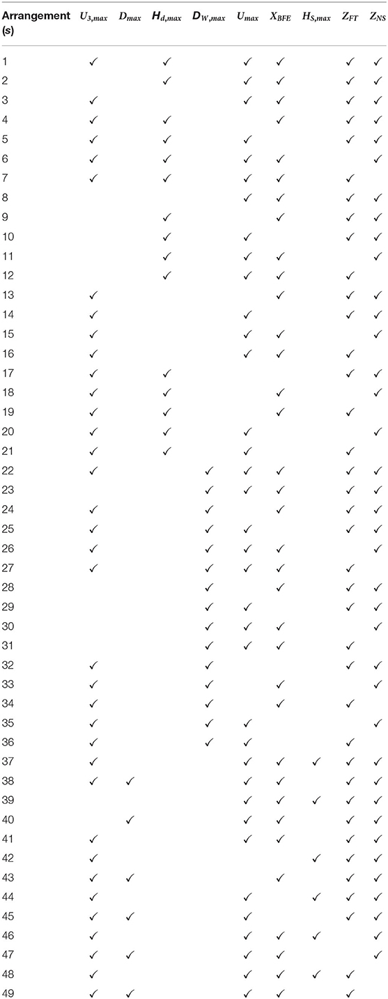
Table 4. Arrangements (S) with main explanatory variables.

For screening purposes, two rejection criteria are used to evaluate the fit of the models. These criteria are (1) satisfaction of model requirements (satisfying of proportional odds assumption for proportional odds cumulative logit model and goodness-of-fit logistic regression model) and (2) statistical significance of model parameters (at least one model variable should be statistically significant or the model is rejected). Among the 539 models, models satisfying criterion 1 are evaluated for criterion 2. Models satisfying the two criteria are then refitted based on Equations (2) and (6) to include interactions and reevaluated based on criterion 1. Once models pass criterion 1, models are assessed based on two other assessment criteria to evaluate the fit and prediction of the models with interaction terms. The assessment criteria are described as (a) statistical significance of model parameters (all interaction terms included in the model must be significant or the model is rejected) and (b) balance between CCR and class error (models with high value of CCR but with high value of CE are considered less reasonable models for damage prediction).

Model Validation

Generally, external cross-validation is used to evaluate the prediction accuracy for logistic regression and proportional odds cumulative logit models. When external data are not available, an alternative approach, known as k-fold cross-validation, is used to assess external prediction. k-fold cross-validation is based on partitioning the dataset into k subsets, with k – 1 subsets used for fitting the model, while the remaining one is used for model validation. For each partition, the model is validated on the remaining one using the model that has fit on all other partitions. In this study, a special case of k-fold cross-validation, known as leave-one-out cross-validation (LOOCV), where k is equal to the sample size (N) is used. Recently, this method has been used to evaluate performance of fragility models for buildings subjected to tsunami (Macabuag et al., 2016), earthquake (Mai et al., 2017), and hurricane hazards (Massarra et al., 2019) and for line towers subjected to wind (Cai et al., 2019). Models satisfied the rejection (criteria 1 and 2) and assessment (criteria a and b) criteria and are fitted N times, leaving one observation out at each fit.

For each fit and for every left-out observations, the predicted DS $(\widehat{DS})$ is then estimated as follows:

• For the logistic regression model, Equation (4) is used to estimate the predicted probability of collapse $(\widehat{p})$. If $\widehat{p}$ is estimated to be <0.5, no collapse is assigned as the predicted DS $(\widehat{DS})$; otherwise, collapse is assigned.

• For the proportional odds cumulative logit models, Equation (9) is used to estimate probabilities that a DS fall into any specific damage level J. Based on the calculated estimated probabilities, DS corresponding to the highest estimated probability is assigned as the predicted DS $(\widehat{DS})$.

For every left-out observation, an error matrix with N observations, d rows, and c columns is then constructed. The frequency (k) of observed DS is represented by rows (d), while the frequency of predicted DS $(\widehat{DS})$ is represented by columns (c), summed across the N left-out observations. The cross-classification rate (CCR), which represents the percentage of correctly classified damage states, is calculated as $CCR=\frac{\sum _{c=1}^C{k}_{cc}}{\sum _{c=1}^C\sum _{d=1}^D{k}_{cd}}$, where k_cc are observations along the diagonal of the error matrix, and k_cd are all observations in the error matrix. Class error (CE), which represents the percentage of each misclassified DS, is calculated as $CE=1-\frac{k_{cc}}{\sum _{c=1}^C{k}_{cd}}$.

Results

Fragility Fitting

Based on Equations (1) and (5), respectively, models 10 and 8, with main explanatory variables (U_3,max, H_S,max, Z_FT, Z_NS) satisfied criteria 1 and 2 (Table 5), while the rest of the models failed to satisfy criterion 1 and were not evaluated for criterion 2. To include HA interactions, models 8, and 10 were refitted based on Equations (6) and (2), respectively, and evaluated based on criteria 1 and a. Table 6 describes variables used to fit models that satisfied criteria 1 and a. These models are described with four main explanatory variables (U_3,max, H_S,max, Z_FT, Z_NS) and one interaction term $(H_{S,max}^{*}{Z}_{NS}$). Table 7 contains the parameter estimates, standard error, p-value, factored model coefficients (_Mhβh, _Mhηha), odds ratio (MOR_h ,MOR_ha) calculated based on = exp(_Mhηha), and the corresponding CI_95% (MOR_hCI_95%, MOR_haCI_95%) for models that met criteria 1 and a. Values of M_hβ, _Mhβha, MOR_h, MOR_ha, MOR_hCI_95%, and MOR_haCI_95% were calculated using M_U3,max = 4.5 (m/s), M_HS,max = 0.3 (m), M_Dmax = 1 (m), and M_Umax=0.5 (m/s). Asterisks appearing after p-values denote statistically significant parameters at α = 0.05 level. The subscripts of the coefficients represent, j,h,a, and ha for α, β, γ, and η, respectively, where j,h,a, and ha correspond to j = 1,2,3, h=1, 2, a=1,2, and ha = 2,2.

TABLE 5

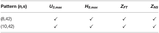
Table 5. Patterns (n,s) with main explanatory variables for models that satisfied criteria 1 and 2.

TABLE 6

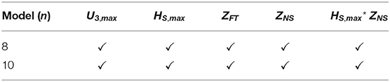
Table 6. Models with main explanatory variables and interaction terms that satisfied criteria 1 and a.

TABLE 7

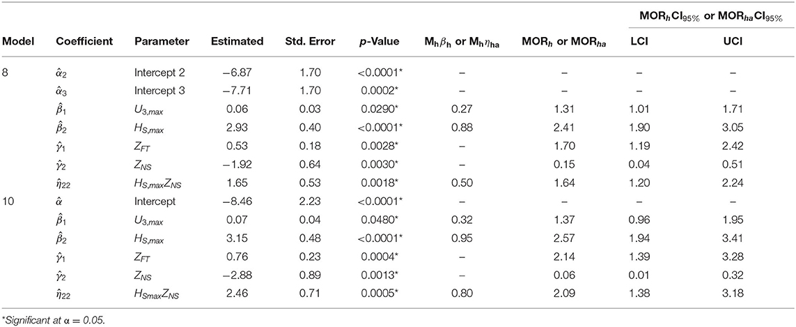
Table 7. Parameter estimates, standard error, p-value, MOR_h, MOR_ha, MOR_hCI_95%, and MOR_haCI_95% for models satisfying criteria 1 and a.

For models 8 and 10, the results show that the damage and collapse of buildings are significantly affected by the maximum 3-s gust wind speed and maximum significant wave height. As any of these hazard variables increase, the odds of being in a higher damage state and collapse increase. Kennedy et al. (2010), Tomiczek et al. (2014a,b), and Tomiczek et al. (2017) also found that wave height significantly contribute to building damage and should be considered as input in the fragility models. However, based on the fact that Hurricanes Ike (2009) and Sandy (2012) were events with low wind speeds, wind speed was excluded from the analyses of these studies. Hurricane Katrina was also an event with low wind speeds; however, the maximum 3-s gust wind speed was found to be a factor that contributes significantly to damage and collapse. The interaction term enabled interpretation of how much the damage differs between one- and two-story buildings with the increasing wave height. The effect of increasing wave height on building damage can be interpreted from the model with just heard parameters. However, how much the damage differs between one- and two-story buildings with the increasing wave height cannot be interpreted from the model with just hazard parameters or building attributes; therefore, models with interaction terms of hazard and building variables are needed.

Since surge depth and surge depth within the building are well-known to be significant factors that affect damage, the significance of these variables in models that failed to satisfy criterion 1 was evaluated. For all these models, it was found that maximum surge depth and surge depth within the building were significant variables that affect damage. Since these models have not satisfied criterion 1, they cannot be considered for further analysis. Inclusion of water speed and base flood elevation in models was also investigated. Results show that either these variables are not significant factors that affect damage, or these variables are significant factors, but models failed to satisfy criterion 1.

Interpretation of Main Effects of DS and Collapse Fragility Models

For model 8, the results show that the damage of buildings are significantly affected by the maximum 3-s gust wind speed and maximum significant wave height. As any of these hazard variables increase, the odds of being in a higher rather than in a lower damage state increase. Interpretation of the odds for maximum 3-s gust wind speed, maximum significant wave height, foundation, and number of stories main effects are as follows:

• For every 4.5 m/s (10.07 mph) increase in maximum 3-s gust wind speed, the odds of being in a higher DS are 1.31 times greater (31% increase in odds), holding all other variables constant.

• For every 0.3 m (0.98 ft) increase in maximum significant wave height, the odds of being in a higher DS are 2.41 times greater (141% increase in odds), holding all other variables constant.

• For buildings with slab foundations, the odds of being in a higher DS are 1.70 times greater (70% increase in odds) than for buildings with elevated foundations, holding all other variables constant.

• For two-story buildings, the odds of being in a higher DS are 0.15 times lower (75% decrease in odds) than for one-story buildings, holding all other variables constant.

For the logistic model (model 10), the results show that the collapse potential of buildings is significantly affected by maximum 3-s gust wind speed and maximum significant wave height. As any of these hazard variables increase, the odds of collapse increase. Interpretation of the odds for maximum 3-s gust wind speed, maximum significant wave height, foundation, and number of stories main effects are as follows:

• For every 4.5 m/s (10.07 mph) increase in maximum 3-s gust wind speed, the odds of being in a higher DS are 1.37 times greater (37% increase in odds), holding all other variables constant.

• For every 0.3 m (0.98 ft) increase in maximum significant wave height, the odds of being in a higher DS are 2.57 times greater (157% increase in odds), holding all other variables constant.

• For buildings with slab foundations, the odds of being in a higher DS are 2.14 times greater (114% increase in odds) than for buildings with elevated foundations, holding all other variables constant.

• For two-story buildings, the odds of being in a higher DS are 0.06 times lower (94% decrease in odds) than for one-story buildings, holding all other variables constant.

Interpretation of Interaction Terms of DS and Collapse Fragility Models

For models 8 and 10, the results show that as maximum significant wave height increase, the odds of being in a higher DS and the odds of collapse are greater for one- than for two-story building. Figures 2A,B show estimated odds MOR_h|Z_{a, 1}, MOR_h|Z_{a, 0} (i.e., numerator and denominator of Equation 13) and the LCI and UCI for models 8 and 10, respectively. The ratio MOR_h|Z_{a, 1} to MOR_h|Z_{a, 0} is equal to MOR_ha shown in Table 7. For model 8, MOR_{HS, max, ZNS} shown in Table 7 equals to 1.64. This is interpreted as follows: for every 0.3 m (0.98 ft) increase in maximum significant wave height, the odds of being in a higher DS are 1.64 times greater for one- rather than for two-story buildings holding all other variables constant. MOR_{HS, max, ZNS} may also be calculated from Figure 2A as ${\text{MOR}}_{H{S}_{,max},Z_{NS}}=\frac{{\text{MOR}}_{H{S}_{,max}|Z_{NS,1}}}{{\text{MOR}}_{H{S}_{,max}|Z_{NS,0}}}$, where MOR_{HS, max|ZNS, 1}and MOR_{HS, max|ZNS, 0} are interpreted as follows: for every 0.3 m (0.98 ft) increase in maximum significant wave height, the odds of being in a higher DS is 3.95 and 2.41 for one- and two-story buildings, respectively, holding all other variables constant.

FIGURE 2

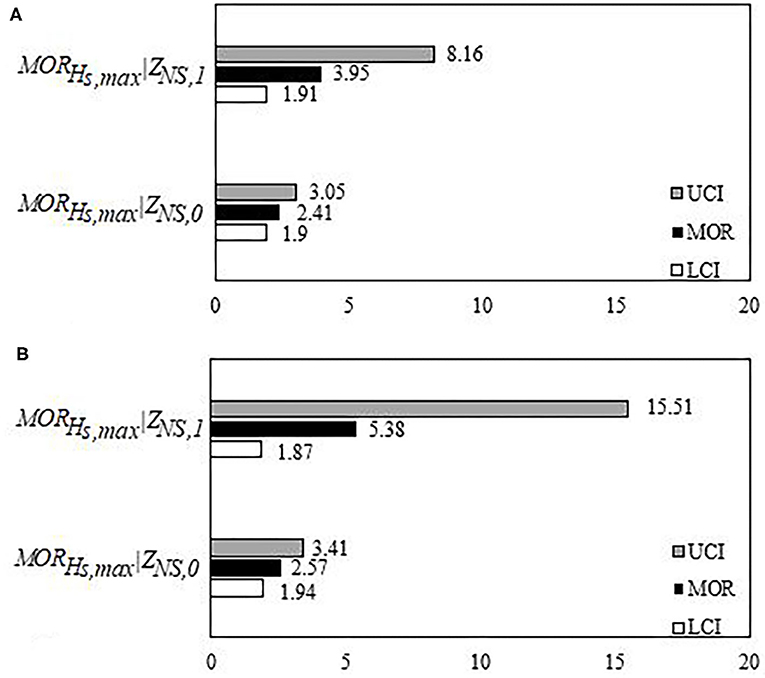
Figure 2. Estimated odds MOR_h|Z_{a, 0}, MOR_h|Z_{a, 1}, and 95% lower (LCI) and upper confidence intervals (UCI) for (A) model 8 and (B) model 10.

For model 10, MOR_{HS,max, ZNS} shown in Table 7 equals to 2.09. This is interpreted as follows: for every 0.3 m (0.98 ft) increase in maximum significant wave height, the odds of collapse are 2.09 times greater for one- rather than for two-story buildings, holding all other variables constant. MOR_{HS, max, ZNS} may also be calculated from Figure 2B as ${\text{MOR}}_{H{S}_{,max},Z_{NS}}=\frac{{\text{MOR}}_{H{S}_{,max}|Z_{NS,1}}}{{\text{MOR}}_{H{S}_{,max}|Z_{NS,0}}}$, where MOR_{HS, max|ZNS, 1}and MOR_{HS, max|ZNS, 0} are interpreted as for every 0.3 m (0.98 ft) increase in maximum significant wave height, the odds of being in a higher DS is 5.38 and 2.57 for one- and two-story buildings, respectively, holding all other variables constant.

Error matrices, with rows representing the frequency of observed DS and columns representing the frequency of predicted DS $(\widehat{DS})$, are provided in Table 8 for models 8 and 10; the n subscript in $({\widehat{DS}}_n)$ represents the corresponding model number. Model 8 predicts the probability of being in or exceeding damage state with 84% prediction accuracy as a function of maximum 3-s gust wind speed, maximum significant wave height, foundation type, number of stories, and interaction of number of stories with maximum significant wave height. DS_1,8 represents no damage or very minor damage to severe damage, DS_2,8 represents very severe damage to partial collapse, and DS_3,8 represents collapse. For model 8, CE for DS_2,8 is high >50%. This increase in CE may be due to the low sample numbers in WF0, WF1, WF4, and WF5 for these DS and groupings of these DS.

TABLE 8

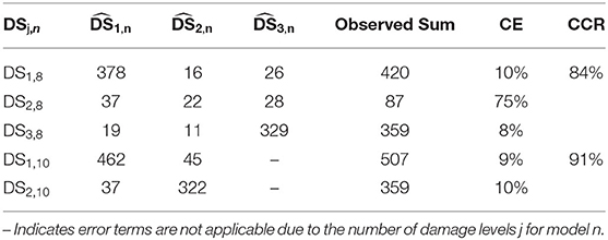
Table 8. Observed vs. predicted model error matrices, class error (CE), and cross-classification rate (CCR) for non-rejected models.

The high CE for DS₂ requires more investigation. Therefore, sensitivity, specificity, positive likelihood ratio (PLR), and negative likelihood ratio (NLR) values were calculated on the confusion matrix. Sensitivity and specificity are useful if the values are high. High sensitivity values mean that it is unlikely that the prediction models are unlikely to predict that a building belongs to a certain DS when the building does not have this DS. High specificity values mean that the prediction models are unlikely to predict false DS for the building when the building does not have this DS. PLR represents the odds of a positive prediction (predicting certain DS) given that the building belongs to this DS, and NLR represents the odds of a positive prediction (predicting a certain DS) given that the building does not belong to this DS. The desirable values are high PLR and low NLP. Sensitivity and specificity of DS₁, DS₂, and DS₃ are (0.90, 0.25, 0.92) and (0.92, 0.98, 0.93), respectively. DS₁ and DS₃ have high sensitivity and specificity, while DS₂ has high and low specificities; therefore, PLR and NLR values are needed. PLR and NLR of DS₁, DS₂, and DS₃ are (11.25, 12.5, 13.15) and (0.09, 0.76, 0.08), respectively. The calculated PLR values are >10; therefore, the model contribution in predicting the three categories is good (Jaeschke et al., 1994). Despite the fact that CE for DS₂ is high (>50%), the calculated PLR values show that the DS model is valid and acceptable; however, future work is recommended to further validate the prediction accuracy of the model on new datasets. The estimated probability of being in or exceeding DS_2,9 and DS_3,9, respectively, is estimated as

$\begin{array}{l}\text{logit}\left[P(Y\ge D{S}_{2,8})\right]=-6.87+0.06^{*}{U}_{3,max}+2.93^{*}{H}_{S,max}\\ +0.53^{*}{Z}_{FT}-1.92^{*}{Z}_{NS}+1.65^{*}{H}_{S,max}{Z}_{NS},& (14)\end{array}$

$\begin{array}{l}\text{logit}\left[P(Y\ge D{S}_{3,8})\right]=-7.71+0.06^{*}{U}_{3,max}+2.93^{*}{H}_{S,max}\\ +0.53^{*}{Z}_{FT}-1.92^{*}{Z}_{NS}+1.65^{*}{H}_{S,max}{Z}_{NS}.& (15)\end{array}$

Model 10 predicts probability of collapse with 91% prediction accuracy as a function of maximum 3-s gust wind speed, maximum significant wave height, foundation type, number of stories, and interaction of number of stories with maximum significant wave height. The estimated probability of collapse is given as

$\begin{array}{l}\text{logit}\left[P(Y\ge D{S}_{10,2})\right]=-8.46+0.07^{*}{U}_{3,max}+3.15^{*}{H}_{S,max}\\ +0.76^{*}{Z}_{FT}-2.88^{*}{Z}_{NS}+2.46^{*}{H}_{S,max}{Z}_{NS}.& (16)\end{array}$

Current models are more comprehensive than other models, with only hazard parameters including previous models developed by the authors (Massarra et al., 2019). The models predict the probability of being in or exceeding a certain damage state and probability of collapse as a function of hazard parameters, building attributes, and their interactions and explain the effect of these variables and their interactions on damage that cannot be explained by fragility models based on just hazard parameters. The prediction accuracy of the developed models is 84 and 91%, respectively, which is a 3% increase in accuracy than the previous models developed by the authors. However, the introduction of the building attributes and interactions of hazard and building attribute variables are not the reason behind this increase. The current developed models are still valid even if the prediction accuracy is less than those with only the hazard parameters.

Study Limitations

The paper does not intend to holistically describe the damage caused by Hurricane Katrina but rather is limited to damage caused to one- and two-story wood-framed single family homes in coastal Mississippi with slab and elevated foundations subjected to wind, wave, and storm surge hazards during 2005 Hurricane Katrina. Higher wind speeds, wave heights, and surge depths and velocities may have occurred as a result of Hurricane Katrina in locations outside the study area, but these are not considered in this paper. Although the hurricane wind field extends far beyond the surge inundation extents, this paper focuses on the multihazard hurricane environment. Many excellent papers on residential building performance and fragility functions for high winds exist (e.g., Li and Ellingwood, 2006; Vickery et al., 2006; van de Lindt et al., 2007; van de Lindt and Dao, 2009), and these should be consulted outside of the multihazard area that is the focus of this paper. Further, as the buildings within the study area were subjected to wind, wave, and surge hazards, we hypothesize that the DS is higher than would be expected if only the wind hazard was considered. Given the relative range of hazards in this study, wave, or storm surge hazard variables were statistically significant predictors of building damage, with problematic multicollinearity between the two, precluding their simultaneous representation in a single model.

Wind hazards are widely acknowledged to cause more damage than any other natural hazard in the US (Emanuel et al., 2006; Knutson et al., 2010; Wang and Rosowsky, 2012). Application of the methodology developed in this paper to future multihazard hurricane events is reasonably expected to result in different model coefficients, but the new results will not contradict the current results. While the presented models are robustly developed and validated, care needs to be taken in interpreting the models and results, and the findings may not be extrapolated beyond the hazard range experienced, as they are not applicable for events with higher wind speeds, wave heights, or surge depths. Because of the limited hazard intensity range and specific building attributes available for model development, the developed models are valid only in this region and other regions with the same building types that are subjected to the same range of hazard intensities defined in this study. Therefore, the developed fragility models are predicated upon building type and hazard intensity rather than the specific study area. At the time of the data collection, no specific sampling technique was implemented. Therefore, a degree of uncertainty is inherent in the data collection and damage assessment that is not considered in this analysis. It is noted that, although this is a major source of uncertainty, this is acknowledged as a significant limitation present across the field of post-disaster reconnaissance and that merits consideration in future studies.

Summary and Conclusions

In this paper, physical damage of one- and two-story wood-framed residential buildings built on slab and elevated foundations in coastal areas was statistically modeled as a function of maximum 3-s gust wind speed, maximum significant wave height, maximum surge depth, maximum water speed, foundation type, number of stories, and two-factor interactions of hazard and building attribute variables. The proportional odds cumulative logit model was used to estimate the probability of being in or exceeding three levels of DS described as (1) no damage or very minor damage to severe damage, (2) very severe damage to partial collapse, and (3) collapse, and logistic regression model was used to estimate the probability of collapse.

The developed models identified the variables that have the most significant effect on damage and collapse, while the interaction terms explained the variation of the effect of hazard parameters on the building damage based on levels of building attribute. For DS (model 8) and collapse (model 10) models, maximum 3-s gust wind speed and maximum significant wave height were found to be significant hazard parameters that affect building damage and collapse. Additionally, buildings with slab foundations were more likely to be in a higher damage state or collapse than elevated buildings. The interaction of maximum significant wave height with number of stories was statistically significant and showed that damage for one-story buildings increases significantly than that for two-story buildings with increasing wave height, where for a certain increase in maximum significant wave height (0.3 m used in this study), one-story buildings were more likely to be in a higher damage state or collapse than two-story buildings.

Maximum surge depth was found to be a significant predictor for damage and collapse in all models that include this variable; however, none of these models satisfied criterion 1 (model requirements) and were excluded from further analyses. Base flood elevation, maximum significant wave depth, maximum surge depth within the building, and interaction between surge depth and foundation type and between wind speed and number of stories were found to be significant predictors for damage and collapse in some models; however, these models were excluded from further analyses because the models did not satisfy criterion 1 (model requirements).

The methodology developed in this paper is useful for researchers, coastal engineers, insurance companies, and model developers who rely on field data more than simulated data. Models developed in this study are more comprehensive than those with only hazard parameters and explain how the significant interaction between hazard and building attributes reflect variation in hazard effect on damage based on the levels of building attributes. Models that consider only hazard parameters are useful when detailed information about the study area buildings is not available (e.g., quick planning exercises, pre-event forecasting), while models that consider both hazard and building attributes provide greater detail about the performance of buildings based on damage indicator variables. These models can be used and are appropriate when detailed inventory data are available. The LOOCV used in this study is a vital advantage over data-based fragility models found in the literature, where these models have been developed for inference and interpretation of model coefficients rather than for future damage prediction. It is anticipated that future work will use the same methodology with the inclusion of the location, first floor elevation, and construction age as input variables to identify the effect of these variables on damage and collapse.

Additionally, continued investigation of the performance of the models presented here on other datasets that have the same characteristic of this dataset will yield increased understanding about model prediction capability. A sampling technique to obtain a sample representative of all damages in the area and an extension of methodology to estimate damage to exterior components such as roof, wall, openings, and foundation remain subjects for future work.

Data Availability Statement

The datasets generated for this study are available on request to the corresponding author.

Author Contributions

CM designed the model, analyzed the data, interpreted the results, and drafted the manuscript in consultation with the co-authors. CF and BM critically revised the manuscript and provided comprehensive feedback. BM critically revised the manuscript and provided comprehensive feedback on model development and interpretation. JD provided the computational hazard data, wrote the section of the manuscript Simulated Explanatory Hazard Variables Hazard, revised the manuscript and provided feedback. All authors contributed to the article and approved the submitted version.

Conflict of Interest

The authors declare that the research was conducted in the absence of any commercial or financial relationships that could be construed as a potential conflict of interest.

Acknowledgments

The authors gratefully acknowledge funding from the Louisiana Board of Regents Graduate Fellowship in Engineering Grant No. LEQSF (2008-13) GF-01, the Donald W. Clayton Graduate Ph.D. Assistantship in Engineering, and the Chevron Engineering Graduate Student Fellowship. Hurricane Katrina reconnaissance videos were provided by MCEER (http://www.buffalo.edu/mceer.html).

References

Adams, B. J., Huyck, C., Mio, M., Cho, S., Eguchi, R. T., Womble, A., and Mehta, K. (2004). “Streamlining post-disaster data collection and damage assessment, using VIEWS (visualizing impacts of earthquakes with satellites) and VRS (virtual reconnaissance system),” in Paper Presented at the Proceedings of 2nd International Workshop on Remote Sensing for Post-Disaster Response (Newport Beach, CA).

Booij, N., Ris, R., and Holthuijsen, L. H. (1999). A third-generation wave model for coastal regions: 1. Model description and validation. J. Geophys. Res. 104, 7649–7666. doi: 10.1029/98JC02622

CrossRef Full Text | Google Scholar

Cai, Y., Xie, Q., Xue, S., Hu, L., and Kareem, A. (2019). Fragility modelling framework for transmission line towers under winds. Eng. Struct. 191, 686–697. doi: 10.1016/j.engstruct.2019.04.096

CrossRef Full Text | Google Scholar

Cardone, V. J., Cox, A. T., and Forristall, G. Z. (2007). “Hindcast of winds, waves and currents in northern Gulf of Mexico in Hurricanes Katrina (2005) and Rita (2005),” in Paper Presented at the Offshore Technology Conference (Houston, TX).

Google Scholar

Charvet, I., Ioannou, I., Rossetto, T., Suppasri, A., and Imamura, F. (2014a). Empirical fragility assessment of buildings affected by the 2011 great east Japan tsunami using improved statistical models. Nat. Hazards 73, 951–973. doi: 10.1007/s11069-014-1118-3

CrossRef Full Text | Google Scholar

Charvet, I., Suppasri, A., and Imamura, F. (2014b). Empirical fragility analysis of building damage caused by the 2011 great east Japan tsunami in Ishinomaki city using ordinal regression, and influence of key geographical features. Stoch. Environ. Res. Risk Assess. 28, 1853–1867. doi: 10.1007/s00477-014-0850-2

CrossRef Full Text | Google Scholar

Charvet, I., Suppasri, A., Kimura, H., Sugawara, D., and Imamura, F. (2015). A multivariate generalized linear tsunami fragility model for Kesennuma City based on maximum flow depths, velocities and debris impact, with evaluation of predictive accuracy. Nat. Hazards 79, 2073–2099. doi: 10.1007/s11069-015-1947-8

CrossRef Full Text | Google Scholar

Curtis, A., Duval-Diop, D., and Novak, J. (2010). Identifying spatial patterns of recovery and abandonment in the post-katrina holy cross neighborhood of New Orleans. Cartogr. Geogr. Inf. Sci. 37, 45–56. doi: 10.1559/152304010790588043

CrossRef Full Text | Google Scholar

Curtis, A., Mills, J. W., Kennedy, B., Fotheringham, S., and McCarthy, T. (2007a). Understanding the geography of post-traumatic stress: an academic justification for using a spatial video acquisition system in the response to hurricane katrina. J. Contingencies Crisis Manag. 15, 208–219. doi: 10.1111/j.1468-5973.2007.00522.x

CrossRef Full Text | Google Scholar

Curtis, A., Mills, J. W., and Leitner, M. (2007b). Katrina and vulnerability: the geography of stress. J. Health Care Poor Underserved. 18, 315–330. doi: 10.1353/hpu.2007.0029

PubMed Abstract | CrossRef Full Text | Google Scholar

Dietrich, J. C., Bunya, S., Westerink, J., Ebersole, B., Smith, J., Atkinson, J., et al. (2010). A high-resolution coupled riverine flow, tide, wind, wind wave, and storm surge model for southern Louisiana and Mississippi. Part II: Synoptic description and analysis of Hurricanes Katrina and Rita. Monthly Weather Rev. 138, 378–404. doi: 10.1175/2009MWR2907.1

CrossRef Full Text | Google Scholar

Dietrich, J., Tanaka, S., Westerink, J. J., Dawson, C., Luettich, R. Jr., Zijlema, M., et al. (2012b). Performance of the unstructured-mesh, SWAN+ ADCIRC model in computing hurricane waves and surge. J. Sci. Comput. 52, 468–497. doi: 10.1007/s10915-011-9555-6

CrossRef Full Text | Google Scholar

Dietrich, J., Trahan, C., Howard, M., Fleming, J., Weaver, R., Tanaka, S., et al. (2012a). Surface trajectories of oil transport along the northern coastline of the Gulf of Mexico. Cont. Shelf Res, 41, 17–47. doi: 10.1016/j.csr.2012.03.015

CrossRef Full Text | Google Scholar

Emanuel, K., Ravela, S., Vivant, E., and Risi, C. (2006). A statistical deterministic approach to hurricane risk assessment. Bullet. Am. Meteorol. Soc. 87, 299–314. doi: 10.1175/BAMS-87-3-299

CrossRef Full Text | Google Scholar

Friedland, C. J., and Levitan, M. L. (2009). “Loss-consistent categorization of hurricane wind and storm surge damage for residential structures,” Paper presented at the Proceedings of the 11th Americas Conference on Wind Engineering (San Juan).

Google Scholar

Hatzikyriakou, A. (2017). Vulnerability and hazard modeling for coastal flooding due to storm surge (Ph.D. dissertation), Princeton University, Princeton, NJ, United States.

Google Scholar

Hatzikyriakou, A., and Lin, N. (2018). Assessing the vulnerability of structures and residential communities to storm surge: an analysis of flood impact during hurricane sandy. Front. Built. Environ. 4:4. doi: 10.3389/fbuil.2018.00004

CrossRef Full Text | Google Scholar

Hatzikyriakou, A., Lin, N., Gong, J., Xian, S., Hu, X., and Kennedy, A. (2015). Component-based vulnerability analysis for residential structures subjected to storm surge impact from hurricane sandy. Nat. Hazards Rev. 17:205. doi: 10.1061/(ASCE)NH.1527-6996.0000205

CrossRef Full Text | Google Scholar

Jaccard, J., and Turrisi, R. (2003). Interaction Effects in Multiple Regression. Newbury Park, CA: Sage.

Google Scholar

Jaeschke, R., Guyatt, G. H., Sackett, D. L., Guyatt, G., Bass, E., Brill-Edwards, P., et al. (1994). Users' guides to the medical literature: III. How to use an article about a diagnostic test B. What are the results and will they help me in caring for my patients? JAMA Netw. 271, 703–707. doi: 10.1001/jama.271.9.703

PubMed Abstract | CrossRef Full Text | Google Scholar

Kameshwar, S., and Padgett, J. E. (2018). Fragility and resilience indicators for portfolio of oil storage tanks subjected to hurricanes. J. Infrastruct. Syst. 24:04018003. doi: 10.1061/(ASCE)IS.1943-555X.0000418

CrossRef Full Text | Google Scholar

Kennedy, A., Rogers, S., Sallenger, A., Gravois, U., Zachry, B., Dosa, M., et al. (2010). Building destruction from waves and surge on the bolivar peninsula during hurricane ike. J. Waterway Port Coast. Ocean Eng. 137, 132–141. doi: 10.1061/(ASCE)WW.1943-5460.0000061

CrossRef Full Text | Google Scholar

Knutson, T. R., McBride, J. L., Chan, J., Emanuel, K., Holland, G., Landsea, C., et al. (2010). Tropical cyclones and climate change. Nat. Geosci. 3, 157–163. doi: 10.1038/ngeo779

CrossRef Full Text | Google Scholar

Koshimura, S., Namegaya, Y., and Yanagisawa, H. (2009). Tsunami fragility: a new measure to identify tsunami damage. J. Disaster Res. 4, 479–488. doi: 10.20965/jdr.2009.p0479

CrossRef Full Text | Google Scholar

Lallemant, D., Kiremidjian, A., and Burton, H. (2015). Statistical procedures for developing earthquake damage fragility curves. Earthquake Eng. Struct. Dynamics. 44, 1373–1389. doi: 10.1002/eqe.2522

CrossRef Full Text | Google Scholar

Li, Y., and Ellingwood, B. R. (2006). Hurricane damage to residential construction in the US: importance of uncertainty modeling in risk assessment. Eng. Struct. 28, 1009–1018. doi: 10.1016/j.engstruct.2005.11.005

CrossRef Full Text | Google Scholar

Lillesand, T., Kiefer, R. W., and Chipman, J. (2014). Remote Sensing and Image Interpretation. New York, NY: John Wiley & Sons.

Google Scholar

Lue, E., Wilson, J. P., and Curtis, A. (2014). Conducting disaster damage assessments with spatial video, experts, and citizens. Appl. Geogr. 52, 46–54. doi: 10.1016/j.apgeog.2014.04.014

CrossRef Full Text | Google Scholar

Luettich, R. A., and Westerink, J. J. (2004). Formulation and numerical implementation of the 2D/3D ADCIRC finite element model version 44. XX. Retrieved from https://adcirc.org/adcirc_theory_2004_12_08.pdf

Google Scholar

Macabuag, J., Rossetto, T., Ioannou, I., Suppasri, A., Sugawara, D., Adriano, B., et al. (2016). A proposed methodology for deriving tsunami fragility functions for buildings using optimum intensity measures. Nat. Hazards 84, 1257–1285. doi: 10.1007/s11069-016-2485-8

CrossRef Full Text | Google Scholar

Mai, C., Konakli, K., and Sudret, B. (2017). Seismic fragility curves for structures using non-parametric representations. Front. Struct. Civil Eng. 11, 169–186. doi: 10.1007/s11709-017-0385-y

CrossRef Full Text | Google Scholar

Massarra, C. C., Friedland, C. J., Marx, B. D., and Dietrich, J. C. (2019). Predictive multi-hazard hurricane data-based fragility model for residential homes. Coast. Eng. 151, 10–21. doi: 10.1016/j.coastaleng.2019.04.008

CrossRef Full Text | Google Scholar

Muhari, A., Charvet, I., Tsuyoshi, F., Suppasri, A., and Imamura, F. (2015). Assessment of tsunami hazards in ports and their impact on marine vessels derived from tsunami models and the observed damage data. Nat. Hazards 78, 1309–1328. doi: 10.1007/s11069-015-1772-0

CrossRef Full Text | Google Scholar

Nateghi, R., Guikema, S. D., and Quiring, S. M. (2011). Comparison and validation of statistical methods for predicting power outage durations in the event of hurricanes. Risk Anal. 31, 1897–1906. doi: 10.1111/j.1539-6924.2011.01618.x

PubMed Abstract | CrossRef Full Text | Google Scholar

Padgett, J. E., Spiller, A., and Arnold, C. (2012). Statistical analysis of coastal bridge vulnerability based on empirical evidence from hurricane katrina. Struct. Infrastruct. Eng. 8, 595–605. doi: 10.1080/15732470902855343

CrossRef Full Text | Google Scholar

Pitilakis, K., Crowley, H., and Kaynia, A. (2014). SYNER-G: Typology Definition and Fragility Functions for Physical Elements at Seismic Risk, Vol. 27. Springer.

Google Scholar

Porter, K., Kennedy, R., and Bachman, R. (2007). Creating fragility functions for performance-based earthquake engineering. Earthquake Spectra 23, 471–489. doi: 10.1193/1.2720892

CrossRef Full Text | Google Scholar

Powell, M. D., Murillo, S., Dodge, P., Uhlhorn, E., Gamache, J., Cardone, V., et al. (2010). Reconstruction of Hurricane Katrina's wind fields for storm surge and wave hindcasting. Ocean Eng. 37, 26–36. doi: 10.1016/j.oceaneng.2009.08.014

CrossRef Full Text | Google Scholar

Reed, D. A., Friedland, C. J., Wang, S., and Massarra, C. C. (2016). Multi-hazard system-level logit fragility functions. Eng. Struct. 122, 14–23. doi: 10.1016/j.engstruct.2016.05.006

CrossRef Full Text | Google Scholar

Reese, S., Bradley, B. A., Bind, J., Smart, G., Power, W., and Sturman, J. (2011). Empirical building fragilities from observed damage in the 2009 South Pacific Tsunami. Earth-Sci. Rev 107, 156–173. doi: 10.1016/j.earscirev.2011.01.009

CrossRef Full Text | Google Scholar

Reese, S., Cousins, W., Power, W., Palmer, N., Tejakusuma, I., and Nugrahadi, S. (2007). Tsunami vulnerability of buildings and people in South Java–field observations after the July 2006 Java tsunami. Nat. Hazards Earth Syst. Sci. 7, 573–589. doi: 10.5194/nhess-7-573-2007

CrossRef Full Text | Google Scholar

Suppasri, A., Mas, E., Charvet, I., Gunasekera, R., Imai, K., Fukutani, Y., et al. (2013). Building damage characteristics based on surveyed data and fragility curves of the 2011 great east Japan tsunami. Nat. Hazards 66, 319–341. doi: 10.1007/s11069-012-0487-8

CrossRef Full Text | Google Scholar

Suppasri, A., Mas, E., Koshimura, S., Imai, K., Harada, K., and Imamura, F. (2012). Developing tsunami fragility curves from the surveyed data of the 2011 great east Japan tsunami in sendai and ishinomaki plains. Coast. Engi. 54, 1250008-1-1250008-116. doi: 10.1142/S0578563412500088

CrossRef Full Text | Google Scholar

Tang, C., Zhu, J., Chang, M., Ding, J., and Qi, X. (2012). An empirical–statistical model for predicting debris-flow runout zones in the Wenchuan earthquake area. Quatern. Int. 250, 63–73. doi: 10.1016/j.quaint.2010.11.020

CrossRef Full Text | Google Scholar

Tomiczek, T., Kennedy, A., and Rogers, S. (2014a). Collapse limit state fragilities of wood-framed residences from storm surge and waves during hurricane ike. J. Waterway Port Coast. Ocean Eng. 140, 43–55. doi: 10.1061/(ASCE)WW.1943-5460.0000212

CrossRef Full Text | Google Scholar

Tomiczek, T., Kennedy, A., and Rogers, S. (2014b). Survival analysis of elevated homes on the bolivar peninsula after hurricane ike. Bridges 10, 108–118. doi: 10.1061/9780784412626.010

CrossRef Full Text | Google Scholar

Tomiczek, T., Kennedy, A., Zhang, Y., Owensby, M., Hope, M. E., Lin, N., and Flory, A. (2017). Hurricane damage classification methodology and fragility functions derived from hurricane sandy's effects in coastal New Jersey. J. Waterway Port Coast. Ocean Eng. 143:409. doi: 10.1061/(ASCE)WW.1943-5460.0000409

CrossRef Full Text | Google Scholar

van de Lindt, J. W., and Dao, T. N. (2009). Performance-based wind engineering for wood-frame buildings. J. Struct. Eng. 135, 169–177. doi: 10.1061/(ASCE)0733-9445(2009)135:2(169)

CrossRef Full Text | Google Scholar

van de Lindt, J. W., Graettinger, A., Gupta, R., Skaggs, T., Pryor, S., and Fridley, K. J. (2007). Performance of wood-frame structures during Hurricane Katrina. J. Perf. Construct. Facilities 21, 108–116. doi: 10.1061/(ASCE)0887-3828(2007)21:2(108)

CrossRef Full Text | Google Scholar

Vickery, P. J., Skerlj, P. F., Lin, J., Twisdale Jr, L. A., Young, M. A., and Lavelle, F. M. (2006). HAZUS-MH hurricane model methodology. II: Damage and loss estimation. Nat. Hazards Rev. 7, 94–103. doi: 10.1061/(ASCE)1527-6988(2006)7:2(94)

CrossRef Full Text | Google Scholar

Wang, Y., and Rosowsky, D. V. (2012). Joint distribution model for prediction of hurricane wind speed and size. Struct. Safety, 35, 40–51. doi: 10.1016/j.strusafe.2011.12.001

CrossRef Full Text | Google Scholar

Westerink, J. J., Luettich, R. A., Feyen, J. C., Atkinson, J. H., Dawson, C., Roberts, H. J., et al. (2008). A basin-to channel-scale unstructured grid hurricane storm surge model applied to southern Louisiana. Monthly Weather Rev. 136, 833–864. doi: 10.1175/2007MWR1946.1

CrossRef Full Text | Google Scholar

Zhang, Y., Kennedy, A. B., Tomiczek, T., Yang, W., Liu, W., and Westerink, J. J. (2017). Assessment of hydrodynamic competence in extreme marine events through application of boussinesq–green–naghdi models. Appl. Ocean Res. 67, 136–147. doi: 10.1016/j.apor.2017.06.001

CrossRef Full Text | Google Scholar

Zijlema, M. (2010). Computation of wind-wave spectra in coastal waters with SWAN on unstructured grids. Coast. Eng. 57, 267–277. doi: 10.1016/j.coastaleng.2009.10.011

CrossRef Full Text | Google Scholar

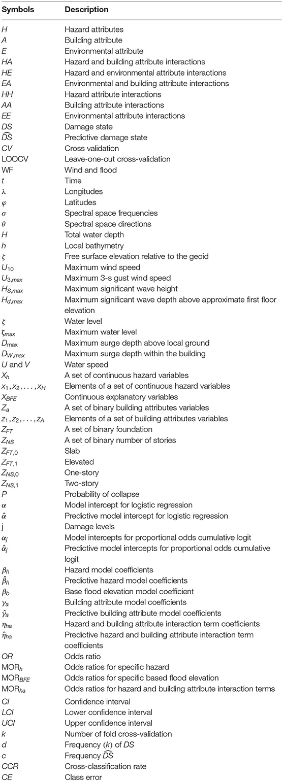
List of Symbols