Mapping Constrained Optimization Problems to Quantum Annealing with Application to Fault Diagnosis

1. Introduction

In the search for ever faster computational substrates, recent attention has turned to devices manifesting quantum effects. Since it has long been realized that computational speedups may be obtained through exploitation of quantum resources, the construction of devices realizing these speedups is an active research area. Currently, the largest scale computing devices using quantum resources are based on physical realizations of quantum annealing. Quantum annealing (QA) is an optimization heuristic sharing much in common with simulated annealing, but which utilizes quantum, rather than thermal, fluctuations to foster exploration through a search space (Finilla et al., 1994; Kadowaki and Nishimori, 1998; Farhi et al., 2000).

QA hardware relies on an equivalence between a physical quantum model and a useful computational problem. The low-energy physics of the D-Wave QA device (Berkley et al., 2010; Harris et al., 2010; Johnson et al., 2011; Dickson et al., 2013) is well captured by a time-dependent Hamiltonian of the form H(t) = A(t)H₀ + B(t)H_P, where ${\mathit{\text{H}}}_0={\sum }_{i\in V\left(G\right)}\mathrm{\sigma }{}_i^x$ includes off-diagonal quantum effects, and where ${\mathit{\text{H}}}_P={\sum }_{i\in V\left(G\right)}{h}_i\mathrm{\sigma }{}_i^z+{\sum }_{\left(i,j\right)\in E\left(G\right)}{J}_{i,j}\mathrm{\sigma }{}_i^z\mathrm{\sigma }{}_j^z$ is used to encode a classical Ising optimization problem of the form

$\underset{\mathit{\text{s}}}{\min }E\left(\mathit{\text{s}}\right)\equiv \underset{\mathit{\text{s}}}{\min }\left\{{\displaystyle \sum _{i\in V(G)}}{h}_i{s}_i+{\displaystyle \sum _{(i,j)\in E(G)}}{J}_{i,j}{s}_i{s}_j\right\}.$ (1)

On the D-Wave device, the connectivity between the binary variables s_i ∈{−1, +1} is described by a fixed sparse graph G = (V, E). The weights J ≡ {J_i,j}_(i,j)∈E(G), and the linear biases h ≡ {h_i}_i∈V(G) are programmable by the user. The A(t) and B(t) functions have units of energy and satisfy B(t = 0) = 0 and A(t = τ) = 0, so that as time advances from t = 0 to t = τ the Hamiltonian H(t) is annealed to a purely classical form. Thus, the easily prepared ground state of H(0) = H₀ evolves to a low-energy state of H(τ) = H_P, and measurements at time τ yield low-energy states of the classical Ising objective equation (1). Theory has shown that if the time evolution is sufficiently slow, i.e., τ is sufficiently large, then with high probability the global minimizer of E(s) can be obtained.

Physical constraints on current hardware platforms (Bunyk et al., 2014) impact this theoretical efficacy of QA. Bian et al. (2014) has noted the following issues that are detrimental to performance:

1. Limited precision/control error on parameters h/J: problems are not represented exactly in hardware, but are subject to small, but noticeable, time-dependent and time-independent additive noise.

2. Limited range on h/J bounds the range of all parameters relative to thermal scales k_bT: thus, very low effective temperatures which are needed for optimization when there are many first excited states are unavailable.

3. Sparse connectivity in G: problems with variable interactions not matching the structure of G cannot be solved directly.

4. Small numbers of total qubits |V(G)|: only problems of up to 1100 variables can currently be addressed.

Bian et al. (2014) suggested approaches ameliorating these concerns. The core idea used to address concerns 1–3 is the construction of penalty representations of constraints with large (classical) energy gaps between feasible and infeasible configurations. The large energy gaps buffer against parameter error and maximize energy scales relative to the fixed device temperature. Sparse device connectivity was addressed using locally structured embedding, which consists of placing constraints directly onto disjoint subgraphs of G and routing constraints together using chains of ferromagnetically coupled qubits representing the same logical variable. This differs from the more common global approach in which constraints are modeled without regard for local hardware structure. We contrast the two approaches in §2.1 and provide some experimental evidence that the locally structured approach is well suited to current QA hardware.

With locally structured embedding, the number of qubits used, size of the energy gaps, and size of chains all play an important role in determining D-Wave hardware performance. Here, we expand on the methods in Bian et al. (2014) and offer several improvements. One way of reducing the required number of qubits, described in §2.2, is by clustering constraints, thereby reducing the number of literals in the CSP. To maximize energy gaps, we follow the methods in Bian et al. (2014) but extend them to max-constraint-satisfaction problems (MAX-CSP): given a set of constraints, find a variable assignment that minimizes the number of constraints that are unsatisfied. §2.3 describes two extensions: one that involves the explicit introduction of variables to indicate the reification of the constraints, and one that does not. Lastly, §2.4 describes how to reduce the size of the largest chains by combining placement and routing of constraints into a single, iterative algorithm. Using linear programing, we also find effective lower bounds on the size of the largest chains, which makes optimal routing faster.

To address the issue of a limited number of total qubits, Bian et al. (2014) adapted two problem decomposition methods to the Ising context, namely dual decomposition (DD) and belief propagation (BP). However, these algorithms suffer from issues of precision and a large number of iterations, respectively. In §2.5, we give two alternatives. One is the well-studied Divide-and-Concur algorithm (Gravel and Elser, 2008), which produces excellent experimental results. The other is a novel message passing algorithm based on distributed minimization of the Bethe free energy called Regional Generalized Belief Propagation; this offers some of the potential benefits of BP with fewer calls to the QA hardware.

A salient feature of D-Wave QA device is the low cost of sampling low-energy configurations of equation (1). After a constant overhead time to program h and J, additional i.i.d. samples can be obtained at an annealing rate of 20 μs/sample. Consequently, problems where a diversity of ground states are sought form an interesting application domain. As an application of our MAX-CSP modeling techniques, we focus on the problem of model-based fault diagnosis. In fault diagnosis, each constraint is realized as a logical gate which defines the input/output pairs allowed by the gate. A circuit of gates then maps global inputs to global outputs. An error model is prescribed for each gate, and fault diagnosis seeks the identification of a minimum number of faulty gates consistent with observed global inputs and outputs and error model. A diversity of minimal cost solutions is valuable in pinpointing the origin of the faults. In §3, we test the ability of the D-Wave hardware to generate a range of minimal cost solutions and also use the hardware to test various decomposition algorithms on a standard benchmark set of fault diagnosis problems.

2. Materials and Methods

2.1. Approaches to Embedding

Modeling a constrained problem as a G-structured Ising objective requires reconciliation of the problem’s structure with that of G. Two approaches may be taken to accommodate the connectivity required by G. In global embedding, we model each constraint as an Ising model without regard for the connectivity of G, add all constraint models, and map the structure of the aggregate model onto G using the heuristic minor-embedding algorithm of Cai et al. (2014). Previous examples of global embedding include Bian et al. (2013), Douglass et al. (2015), Perdomo-Ortiz et al. (2015), Rieffel et al. (2015), Venturelli et al. (2015b), and Zick et al. (2015). Alternatively, when the scopes of constraints are small, locally structured embedding (Bian et al., 2014) models each constraint locally within a subgraph 𝒢 ⊂ G, places the local subgraphs 𝒢 within G, and then connects (routes) variables occurring in multiple local subgraphs. Figure 1 contrasts the two approaches.

FIGURE 1

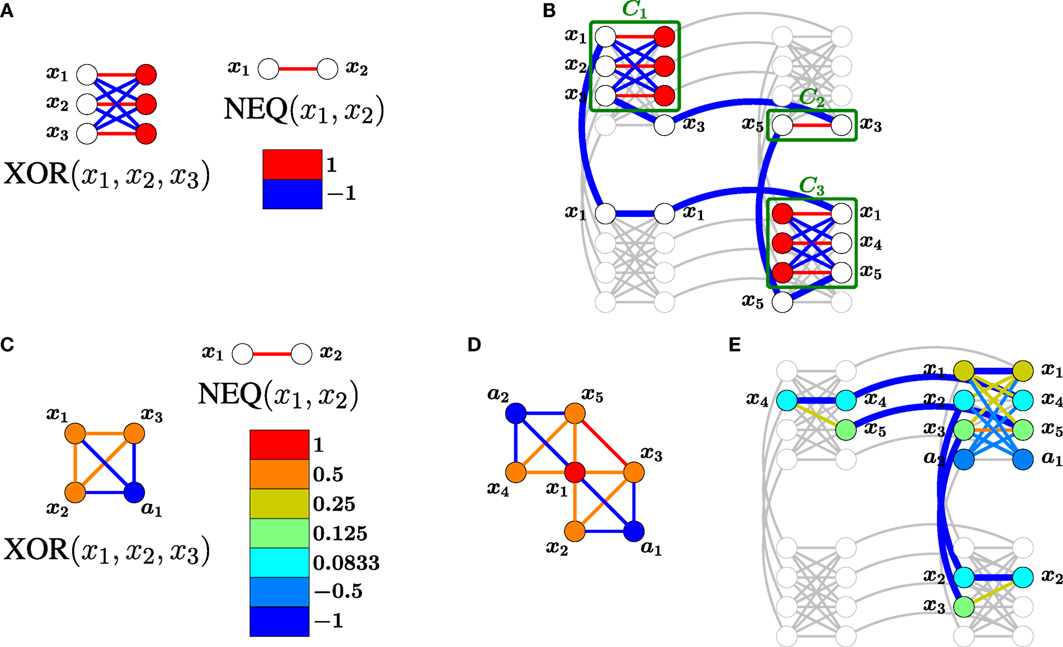
Figure 1. Comparison of locally structured (top) and global (bottom) embeddings of a CSP with constraints {XOR(x₁, x₂, x₃), XOR(x₁, x₄, x₅), NEQ(x₃, x₅)} in a D-Wave-structured hardware graph. (A) The penalty models for XOR and NEQ have an energy gap g = 2. (B) After locally structured embedding with a chain strength of α = 1, the Ising model for the CSP has an energy gap of 2. Chain couplings are indicated with thick blue edges. (C) The given penalty model for XOR using only 4 qubits has energy gap g = 1. (D) The aggregate Ising model for the CSP. Variable a_i is an auxiliary variable used to define the i-th constraint. (E) Global embedding of the aggregate model. The chain strength α = 2 was optimized experimentally, and the entire Ising model is scaled by a factor of 1/α to satisfy the range requirement −1 ≤ J_ij ≤ 1. After scaling, the Ising model for the CSP has an energy gap of g = 0.5. The global embedding uses fewer qubits but requires more precision to specify and has a smaller energy gap.

The methods offer different trade-offs. The former method typically utilizes fewer qubits and has shorter chains of connected qubits representing logical problem variables. The latter method is more scalable to large problems, usually requires less precision on parameters, and offers lower coupling strengths used to enforce chains. More precisely, assume an embedded Ising model is parameterized by [h, J] = [h, J_P + αJ_C], where [h, J_P] describes the encoded constraints, J_C enforces the couplings within chains, and α > 0 is a chain strength. In a satisfiable CSP that has been embedded with the locally structured approach, the chains representing a solution to the CSP will be a ground state of [h, J] regardless of the choice of α.¹ By contrast, for some global embeddings, the chain strength required to enforce unbroken chains can grow with system size, increasing the precision with which the original problem must be represented and making the dynamics of quantum annealing more difficult (Venturelli et al., 2015a).

Whether the benefits of improved precision and lower chain strengths outweigh the drawbacks of using more qubits depends on the problem. Figure 2 gives an example of a problem class (random XOR-3-SAT problems) for which the overall performance and scaling of quantum annealing hardware is noticeably improved with locally structured embedding. For the fault diagnosis problems studied here, the locally structured approach also performs better, and we pursue improvements to the locally structured algorithm of Bian et al. (2014).

FIGURE 2

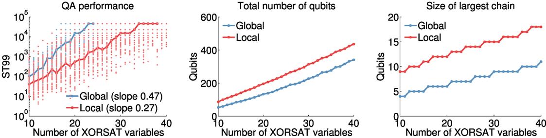
Figure 2. Comparison of the D-Wave quantum annealing hardware performance in solving XOR-3-SAT problems (Jia et al., 2005), using global (blue) and locally structured (red) modeling strategies. Each XOR-3-SAT instance is randomly generated subject to having a unique solution and a clause-to-variable ratio of 1.0. Global embeddings: each constraint $s_1{s}_2{s}_3=1$ (with $s_i=\pm 1$) is encoded in the 4-qubit penalty model in Figure 1C, which has energy gap g = 1. The Ising model representing the sum of these constraints is then embedded using the heuristic in Cai et al. (2014). Local embeddings: each constraint is mapped directly to the K_3,3-structured Ising model in Figure 1A, which has energy gap g = 2. Constraints are then embedded using the rip-up and replace algorithm in §2.4.2. Left: scaling of hardware performance with no post-processing. ST99 is the number of samples needed to find the ground state with 99% probability, which, given a fraction p of all samples taken that are in the ground state, is given by the formula ST99 = log(1 − 0.99)/log(1 − p) (Rönnow et al., 2014). Bold lines indicate the median across 50 instances of each problem size. For points not shown, the hardware failed to find a ground state. Middle: total number of qubits required to embed the Ising model (median). Right: number of qubits in the largest chain in the embedding (median).

2.2. Preprocessing

For some CSPs, aggregating several small constraints into a single larger one prior to modeling may lead to more efficient hardware mappings and better hardware performance. The benefit stems from the fact that variables appearing in multiple constraints within a cluster need only be represented once (or perhaps not at all). As an example, consider the Boolean-valued constraint y = XOR(x₁, x₂). If XOR is represented using AND/OR/NOT gates, for example, as {a₁ = AND(x₁, ¬ x₂), a₂ = AND(x₂, ¬ x₁), y = OR(a₁, a₂)}, at least 9 literals are needed. On the other hand, by clustering the three gates, XOR can be represented by an Ising model directly using only 4 qubits (see Figure 1C).

Unfortunately, as constraints become larger it becomes more difficult to find Ising models to represent them. This upper limit on the practical cluster size requires straightforward modifications to standard clustering methods such as agglomerative clustering (Tan et al., 2005). When the CSP is derived from a combinational circuit, cone-based clustering (Siddiqi and Huang, 2007; Metodi et al., 2014) can also be adapted to accommodate bounds on the cluster size. Both agglomerative and cone clustering can be performed in polynomial time.

2.3. Mapping Constraints to Ising Models

Regardless of whether or not constraints are clustered, the next step in mapping to hardware is identifying an Ising model to represent each constraint. We assume a constraint on n binary variables is characterized by a subset of {0, 1}ⁿ, which indicates valid variable assignments. Since quantum hardware uses spin variables with values in {−1, +1}, we identify 0 with −1 and 1 with +1, and assume that the feasible set F is a subset of {−1, +1}ⁿ. Our goal is to find an Ising model that separates the feasible solutions F from the infeasible solutions {−1, +1}ⁿ\F based on their energy values. In particular, the ground states of the Ising model must coincide with the feasible solutions F. Furthermore, to improve hardware performance, we seek Ising models for which the gap, i.e., the smallest difference in energy between feasible and infeasible solutions, is largest. Note that we are maximizing the energy gap in the final Hamiltonian, rather than the smallest energy gap throughout quantum annealing, which determines the fastest theoretical annealing time in an ideal, zero-temperature environment (Farhi et al., 2000).

Typically, due to both the complexity of the constraint and the sparsity of the hardware graph, the Ising model requires ancillary variables, which also may help to obtain larger gaps. We assume that the allowable interactions in the Ising model are given by an m-vertex subgraph 𝒢 of the hardware graph G, where m ≥ n. The constraint variables are mapped to a subset of n vertices of 𝒢, while the rest of the vertices are associated with h = m − n ancillary variables. For simplicity, we write a spin configuration z ∈ {−1, +1}^m as z = (s, a), meaning that the working variables take the values s, while the ancillary variables are set to a.

The Ising model we seek is given by variables θ = (θ₀, (θ_i)_i∈V(𝒢), (θ_i,j)_{(i,j)∈E(𝒢)}), where θ_i are the local fields h_i, θ_i,j are the couplings J_i,j, and θ₀ represents a constant energy offset (unconstrained). To simplify the notation, for a configuration z we define ϕ(z) = (1, (z_i)_i∈V(𝒢), (z_iz_j)_{(i,j)∈E(𝒢)}). Thus, the energy of z is given by

${\mathbb{E}}_{\mathrm{\theta }}\left(\mathit{\text{z}}\right)=⟨\mathrm{\theta },\mathrm{\varphi }\left(\mathit{\text{z}}\right)⟩.$

The hardware imposes lower and upper bounds on θ, that we denote, respectively, by $\underset{¯}{\theta }$ and $\overline{\mathrm{\theta }}$ (with ${\overline{\mathrm{\theta }}}_0=+\infty$ and ${\underset{¯}{\theta }}_0=-\infty$). Current D-Wave hardware requires h_i ∈ [−2, 2] and J_i,j ∈ [−1, 1].

To separate feasible and infeasible solutions, we require that for some positive gap g:

$\begin{array}{l}\underset{\mathit{\text{a}}}{\min }{\mathbb{E}}_{\mathrm{\theta }}\left(\mathit{\text{s}},\mathit{\text{a}}\right)=0,\forall \mathit{\text{s}}\in \mathit{\text{F}}\text{\hspace{0.17em}and\hspace{0.17em}}\underset{\mathit{\text{a}}}{\min }{\mathbb{E}}_{\mathrm{\theta }}\left(\mathit{\text{s}},\mathit{\text{a}}\right)\ge g,\forall \mathit{\text{s}}\notin \mathit{\text{F}}.\end{array}$ (2)

Thus, the problem of finding the Ising model with largest gap can be stated as follows:

$\begin{array}{ll}\underset{g,\mathrm{\theta }}{\max }& g\\ \text{subject\hspace{0.17em}to}& ⟨\mathrm{\theta },\mathrm{\varphi }\left(\mathit{\text{s}},\mathit{\text{a}}\right)⟩\ge 0\forall \mathit{\text{s}}\in \mathit{\text{F}},\forall \mathit{\text{a}}\end{array}$ (3)

$⟨\mathrm{\theta },\mathrm{\varphi }\left(\mathit{\text{s}},\mathit{\text{a}}\right)⟩\ge g\forall \mathit{\text{s}}\notin \mathit{\text{F}},\forall \mathit{\text{a}}$ (4)

$\begin{array}{lll}\exists \mathit{\text{a}}:& ⟨\mathrm{\theta },\mathrm{\varphi }\left(\mathit{\text{s}},\mathit{\text{a}}\right)⟩=0& \forall \mathit{\text{s}}\in \mathit{\text{F}}\\ & \underset{¯}{\theta }\le \mathrm{\theta }\le \overline{\mathrm{\theta }}.& \end{array}$ (5)

Here, constraints (3) and (5) guarantee that all feasible solutions have minimum energy 0, while constraint (4) forces infeasible solutions to have energy at least g.

This optimization problem is solved as a sequence of feasibility problems with fixed gaps g. Using the fact that the interaction graph 𝒢 has low treewidth, we can significantly condense the formulation above. In this way, the number of constraints may be reduced from exponential in m to exponential in the treewidth of 𝒢. The resulting model is solved with a Satisfiability Modulo Theories (SMT) solver [see Bian et al. (2014) for more details].

The penalty-finding techniques above assume that a placement of variables within the Ising model is given. However, different placements allow for different energy gaps, and it is not clear, even heuristically, what characteristics of a placement lead to larger gaps. For small constraints, canonical augmentation (McKay, 1998) can be used to generate all non-isomorphic placements.

2.3.1. Methods for MAX-CSP

Borrowing from fault diagnosis terminology, we consider constraints characterized by two disjoint subsets of feasible solutions: healthy states F₁ ⊆ {−1, 1}ⁿ, and faulty states F₂ ⊆ {−1, 1}ⁿ. States in {−1, 1}ⁿ \ (F₁ ∪ F₂) are considered infeasible. As before, we require an Ising model that separates feasible from infeasible solutions, but preferring healthy to faulty states whenever possible. The particular case F₂ = {−1, 1}ⁿ \ F₁ corresponds to a MAX-CSP problem, in which a CSP is unsolvable but nonetheless we attempt to maximize the number of constraints satisfied by applying the same penalty to every constraint with a faulty configuration.

One way to model (F₁, F₂) is through reification where a variable representing the truth of the constraint is introduced. This reified, or health, variable is +1 for healthy states and −1 for faulty states. That is, we define a feasible set

$\mathit{\text{F}}=\left\{\left(\mathit{\text{x}},+1\right):\mathit{\text{x}}\in {\mathit{\text{F}}}_1\right\}\cup \left\{\left(\mathit{\text{x}},-1\right):\mathit{\text{x}}\in {\mathit{\text{F}}}_2\right\}\subseteq {\left\{-1,1\right\}}^{n+1},$

and model F using the methods in §2.3. In this case, both solutions in F₁ and F₂ will be equally preferred. To break the tie to favor healthy states, the health variable can be added to the objective function with negative weight.² We call this the explicit fault model.

A second strategy is to modify the optimization problem of §2.3, so that all solutions in F₁ have energy 0, while all solutions in F₂ have energy e > 0 and infeasible solutions have energy at least g > e. In this case, we fix the intermediate energy e and the optimization problem becomes:

$\begin{array}{ll}\underset{\mathrm{\theta },g\ge e}{\max }& g\\ \text{subject\hspace{0.17em}to}& ⟨\mathrm{\theta },\mathrm{\varphi }\left(\mathit{\text{s}},\mathit{\text{a}}\right)⟩\ge 0\forall \mathit{\text{s}}\in {\mathit{\text{F}}}_1,\forall \mathit{\text{a}}\end{array}$ (6)

$⟨\mathrm{\theta },\mathrm{\varphi }\left(\mathit{\text{s}},\mathit{\text{a}}\right)⟩\ge e\forall \mathit{\text{s}}\in {\mathit{\text{F}}}_2,\forall \mathit{\text{a}}$ (7)

$⟨\mathrm{\theta },\mathrm{\varphi }\left(\mathit{\text{s}},\mathit{\text{a}}\right)⟩\ge g\forall \mathit{\text{s}}\notin {\mathit{\text{F}}}_1\cup {\mathit{\text{F}}}_2,\forall \mathit{\text{a}}$ (8)

$\exists \mathit{\text{a:}}⟨\mathrm{\theta },\mathrm{\varphi }\left(\mathit{\text{s}},\mathit{\text{a}}\right)⟩=0\forall \mathit{\text{s}}\in F_1$ (9)

$\begin{array}{lll}\exists \mathit{\text{a:}}& ⟨\mathrm{\theta },\mathrm{\varphi }\left(\mathit{\text{s}},\mathit{\text{a}}\right)⟩=e& \forall \mathit{\text{s}}\in {\mathit{\text{F}}}_2\\ & \underset{¯}{\theta }\le \mathrm{\theta }\le \overline{\mathrm{\theta }}.& \end{array}$ (10)

It is straightforward to adapt the SMT solution methods of Bian et al. (2014) to this problem. We call this the implicit fault model. The implicit model generally requires fewer variables (i.e., qubits). However, care must be taken to ensure that g is large compared with e; otherwise, when adding penalties together, it may be difficult to differentiate several faulty constraints from a single infeasible constraint. In the explicit model, this issue can be avoided by choosing a sufficiently small weight for health variables in the objective function.

2.4. Locally Structured Embedding

Given a method for generating penalties on subgraphs 𝒢, the next steps of locally structured embedding are the placement of 𝒢’s within G, and the routing of chains of interactions between variables occurring in multiple constraints. Bian et al. (2014) suggested adapting VLSI algorithms for placement (Chan et al., 2000; Roy et al., 2005; Kahng et al., 2011) and routing (Kahng et al., 2011; Gester et al., 2013) to accomplish these steps, and in this section, we describe two improvements to that work. First, using routing models, we find a tight lower bound on the size of the largest chain. This bound is combined with search heuristics to speed the discovery of good embeddings. Second, embedding algorithms that utilize placement and routing steps differ in a significant way from their classical VLSI counterparts, and a modification that performs simultaneous placement and routing improves results.

2.4.1. Chain Length Lower Bounds and Improved Routing

The performance of D-Wave’s hardware in solving an embedded Ising model depends heavily on the size of the chains of variables: shorter chains are more likely to yield better performance (Venturelli et al., 2015a). In this section, we focus on routing which minimizes chain lengths. We assume that constraints have already been placed in the hardware [see Bian et al. (2014) for placement methods]. We show how to find tight lower bounds on the maximum chain size in an embedding and provide an effective procedure to improve routing using these bounds.

We first consider bounds for a single chain, which reduces to the well-studied Steiner tree problem. Let T ⊆ V(G) be a set of terminals, i.e., qubits in the hardware graph to which a variable has been assigned during placement. A Steiner tree is a connected subgraph of G that contains all the terminals. The Steiner tree problem consists of finding the smallest (fewest number of nodes) Steiner tree. The non-terminal vertices in a Steiner tree are called Steiner points.

There are several ways to model the Steiner tree problem as a mixed integer linear program (MILP). However, the tightness of the linear program (LP) relaxation will have a significant impact on the time required to find a solution. Here, we consider a formulation whose LP relaxation, known as the bidirected cut relaxation, has an integrality gap of at most 2 (Rajagopalan and Vazirani, 1999). First, we transform G into a directed graph by replacing each edge with two opposite arcs. For each v ∈ V(G)\T, let x_v be a binary variable indicating whether v is part of the Steiner tree. When variables x_v are fixed, the Steiner tree is just a tree spanning T ∪ {v ∈ V(G): x_v = 1}. A tree can be modeled as a multi-commodity transshipment problem: pick any v₀ ∈ T as root, and find a path from v₀ to each of the other |T| − 1 terminals. Concretely, if we define flow variables $f_a^i$ indicating that arc a is on the path from v₀ to terminal i, then an MILP formulation for the Steiner tree problem is

$\left(\text{BCR}\right)\min \mathrm{\sum }_{v\in V\backslash T}{x}_v$

$\begin{array}{l}\hfill \text{subject to}{\displaystyle \sum _{v\to a}}{f}_a^i-{\displaystyle \sum _{a\to v}}{f}_a^i=\left\{\begin{array}{cc}1\hfill & \text{if}v=v_0\hfill \\ -1\hfill & \text{if}v=v_i\in T,i\ne 0\hfill \\ 0\hfill & \text{if}v\notin T\hfill \end{array}\right.\end{array}$ (11)

$\begin{array}{ll}{\displaystyle \sum _{a\to v}}{f}_a^i\le x_v& \forall v\in V\backslash T,i\ne 0\\ 0\le f_a^i\le 1& \forall a,i\ne 0\\ x_v\in \left\{0,1\right\}\hfill & \forall v\in V\backslash T\end{array}$ (12)

Here, constraints (11) are the flow constraints, while the capacity constraints (12) allow flow to be routed only through Steiner points [i.e., v ∈ V(G) with x_v = 1]. The notation v → a (respectively, a → v) refers to all arcs whose tail is v (respectively, whose head is v).

The LP relaxation of program (BCR) above produces very tight lower bounds for a range of Steiner tree problems (Chopra et al., 1992). This MILP can be extended to the full routing problem using different flows for each Steiner tree to be found, with the additional demand that every variable can appear in at most one Steiner tree.

Having access to good bounds on the chain lengths allows for a simple improvement to the routing phase presented in Bian et al. (2014). Assume that we have a heuristic routing algorithm Route(G, 𝒯, M) that takes as input a hardware graph G, a collection of terminal sets 𝒯 = {T_i} for each variable x_i in the CSP, and a maximal allowable chain size M. Then, any successful call to Route(G, 𝒯, M) will provide an upper bound on the maximal chain length no worse than M, while any unsuccessful call provides a lower bound of M + 1. With these bounds we can perform a heuristic binary search for the optimal maximal chain length, and beginning with the good lower bound provided by the LP relaxation of (BCR) will significantly reduce the number of iterations in the search.

2.4.2. Combined Place-and-Route Algorithms

The place-and-route model of embedding, while known to scale well, is often inefficient in maximizing the size of a problem embeddable in a fixed hardware graph. One reason is that in contrast with VLSI design contexts, the resources being negotiated by placement and routing are identical (namely, vertices of G). So, for example, many placement algorithms attempt to pack constraints as tightly as possible, which leaves few neighboring vertices available for routing. For this reason, we have developed a rip-up-and-replace algorithm which combines the placement and routing phases of embedding, using new routing information to update placements and vice versa.

During the course of the algorithm, vertices of G may be temporarily assigned to multiple variables, with penalties weighted according to the number of times a vertex is used. More precisely, at each step of the algorithm, each CSP variable x_i is assigned a chain S_i ⊂ V(G) of vertices; then, the penalty weight of vertex q ∈ V(G) is defined to be ω(q) = α^{|{i:q∈S_i}|} for some fixed α > 1. Each constraint C is given a placement (L_C, v_C) consisting of a location L_C ⊂ V(G) and an assignment of variables to vertices within the location, v_C: V(C) → L_C [where V(C) denotes the set of variables associated with constraint C].

The algorithm iteratively alternates between assigning constraints to locations, and routing variables between constraints (i.e., creating chains). Chains are constructed using a weighted Steiner tree approximation algorithm such as the MST algorithm (Kou et al., 1981) or Path Composition (Gester et al., 2013). Constraint locations are chosen based on a cost function, where the cost of (L, v) depends on the weight of vertices in L and the weight of routing to (L, v), which is approximated by weighted shortest-path distances to existing chains. The algorithm terminates when a valid embedding is found or no improvement can be made. Explicit details are given in Algorithm 1 below.

ALGORITHM 1

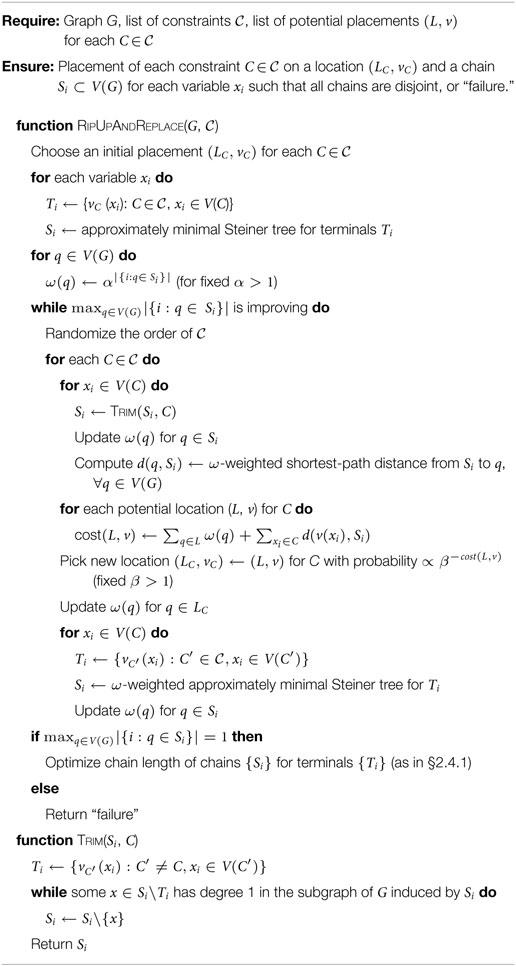
Algorithm 1. Rip-up and replace heuristic for finding a placement of constraints and embedding of variables in a hardware graph.

As an alternative to updating constraint locations based on variable routing, simulated annealing or genetic algorithms can be used to modify placements. For example, define a gene to consist of a preferred location for each constraint, and a priority order for constraints. Given a gene, constraints are placed in order of priority, in their preferred location if it is available or the nearest available location otherwise. During simulated annealing, genes are mutated by perturbing the preferred location for a constraint or transposing two elements in the priority order. These algorithms tend to take much longer than rip-up-and-replace, but eventually produce very good embeddings.

2.5. Decomposition Algorithms

Owing to a limited number of qubits, it is often the case that a CSP or Ising model is too large to be mapped directly onto the hardware. Bian et al. (2014) offered various decomposition techniques which use QA hardware to solve subproblems as a subroutine for solving larger ones. In this section, we describe two additional algorithms: divide-and-concur (Gravel and Elser, 2008; Yedidia, 2011), specialized to our case of Ising model energy minimization, and a new algorithm inspired by regional generalized belief propagation (Yedidia et al., 2005).

For both algorithms, we partition the constraints of a MAX-CSP into regions ℛ = {R₁, R₂, …}, so that each subset of constraints can be mapped to a penalty model on the hardware using the methods of the previous section. For a region R ∈ ℛ, the penalty model [h^(R), J^(R)] produces an Ising energy function E_R(z^(R)) whose ground states satisfy all the constraints in that region. Here, z^(R) is the subset of variables involved in the constraints of region R. Since embedding is slow in general, regions are fixed and embedded in hardware as a preprocessing step.

The key problem with regional decomposition is that sampling a random ground state from each region produces inconsistent settings for variables involved in multiple regions’ constraints. At a high level, messages passed between regions indicate beliefs about the best assignments for variables, and these are used to iteratively update the biases on h^(R) in hopes of converging upon consistent variable assignments across regions. The two algorithms presented here implement this strategy in very different ways.

2.5.1. Divide and Concur (DC)

Divide-and-concur (DC) (Gravel and Elser, 2008; Yedidia, 2011) is a simple message passing algorithm that attempts to resolve discrepancies between instances of variables in different regions via averaging. In each region R, in addition to having an Ising model energy function E_R(z^(R)) representing its constraints, one introduces linear biases L_R(z^(R)) on its variables, initially set to 0. Let $z_i^{\left(R\right)}$ denote the instance of variable z_i in region R. The two phases of each DC iteration are:

• Divide: minimize E_R(z^(R)) + L_R(z^(R)) in each R (i.e., satisfy all constraints and optimize over linear biases).

• Concur: average the instances of each variable: ${\overline{z}}_i={\text{avg}}_{R:z_i\in R}{z}_i^{\left(R\right)}$ and update the linear biases by setting $L_R\left({\mathit{\text{z}}}^{\left(R\right)}\right)={\sum }_{i\in R}-{\overline{z}}_i{z}_i^{\left(R\right)}$.

In the divide phase, E_R is scaled appropriately so that the minimum of E_R(z^(R)) + L_R(z^(R)) satisfies all constraints.

This basic algorithm tends to get stuck cycling between the same states; one mechanism to prevent this problem is to extend DC with difference map dynamics (Yedidia, 2011). DC has been shown to perform well on constraint satisfaction problems and constrained optimization problems, and compared with other decomposition algorithms, has relatively low precision requirements for quantum annealing hardware. That is, assuming each variable is contained in a small number of regions, the linear biases on the variables in the Ising model of each region (namely, $-{\overline{z}}_i$) are discretized. On the other hand, like most decomposition algorithms, DC is not guaranteed to find a correct answer or even converge.

2.5.2. Regional Generalized Belief Propagation (GBP)

Bian et al. (2014) explored min–sum belief propagation as a decomposition method. Here, we take a different approach: instead of minimizing the energy of an Ising model E(z) directly, we sample from its Boltzmann distribution p(z) = e^–E(z)/T/Z. Presuming that we have successfully mapped our constraints to Ising models with large gaps (§2.3), and that the temperature T is sufficiently small, we have confidence that sampling from the Boltzmann distribution provides good solutions to the original constrained optimization problem. The Boltzmann distribution is the unique minimum of the Helmholtz free energy

$A\left(p\right)=U\left(p\right)-\mathrm{TS}\left(p\right)={\displaystyle \sum _z}p\left(\mathit{\text{z}}\right)E\left(\mathit{\text{z}}\right)+T{\displaystyle \sum _z}p\left(\mathit{\text{z}}\right)\log p\left(\mathit{\text{z}}\right).$

Our algorithm decomposes A into regional free energies. The resultant algorithm is similar in spirit to the generalized belief propagation algorithm of Yedidia et al. (2005) based on their region graph method.

Sum–product belief propagation is related to critical points of the (non-convex) Bethe approximation, which for Ising energies reads

$\begin{array}{ll}{A}_{\text{Bethe}}\left(\left\{b_i\right\},\left\{b_{\mathrm{ij}}\right\}\right)=& {\displaystyle \sum _{(i,j)\in E}}{\displaystyle \sum _{z_i,z_j=\pm 1}}{b}_{\mathrm{ij}}\left(z_i,z_j\right)J_{i,j}{z}_i{z}_j+T{b}_{\mathrm{ij}}\left(z_i,z_j\right)\log b_{\mathrm{ij}}\left(z_i,z_j\right)\\ & +{\displaystyle \sum _{i\in V}{\displaystyle \sum _{z_i=\pm 1}}}{b}_i\left(z_i\right)h_i{z}_i+T\left(1-d_i\right)b_i\left(z_i\right)\log b_i\left(z_i\right),\end{array}$

where d_i = |{j ∈ V : (i, j) ∈ E}|. The distribution p in the free energy is approximated by local beliefs (marginals) b_i, b_ij at each vertex and edge. To obtain consistent marginals, $b_i\left(z_i\right)={\sum }_j{b}_{\mathrm{ij}}\left(z_i,z_j\right)$ whenever (i, j) ∈ E, one introduces a constrained minimization problem, and it is the Lagrange multipliers associated with these constraints that relate to the fixed points of belief propagation. In particular, if belief propagation converges then we have produced an interior stationary point of the constrained Bethe approximate free energy (Yedidia et al., 2005).

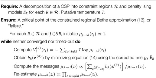
In our case, having divided a MAX-CSP into regions ℛ, we can formulate a regional analog of the Bethe approximation,

$\begin{array}{ll}{A}_{\text{Bethe}}^{\mathcal{R}}\left(\left\{b_i\right\},\left\{b_R\right\}\right)=\hfill & {\displaystyle \sum _{R\in \mathcal{R}}}\left({\displaystyle \sum _{z^{(R)}}}{b}_R\left(z^{\left(R\right)}\right)E_R\left(z^{\left(R\right)}\right)\right.\left.+T{\displaystyle \sum _{z^{(R)}}}{b}_R\left(z^{\left(R\right)}\right)\log b_R\left(z^{\left(R\right)}\right)\right)\hfill \\ \hfill & +T{\displaystyle \sum _i}\left(\left(1-c_i\right){\displaystyle \sum _{z_i}}{b}_i\left(z_i\right)\log b_i\left(z_i\right)\right),\hfill \end{array}$ (13)

where now c_i = |{R: i ∈ R}| is the number of regions whose Ising model includes variable z_i. In exactly the same way as above, requiring consistent marginals induces a constrained minimization problem for this regional approximation. The critical points of this problem are fixed points for a form of belief propagation. Specifically, for each variable z_i in a constraint of R, the messages passed between variable and region are

$\begin{array}{l}{\mu }_{R\to i}\left(z_i\right)\propto {\displaystyle \sum _{z(R)\backslash z_i}}{e}^{-E_R\left({\mathbf{\text{z}}}^{\left(R\right)}\right)∕\mathrm{kT}}{\displaystyle \prod _{j\in R\backslash i}}{\mu }_{j\to R}\left(z_j\right)\\ {\mu }_{i\to R}\left(z_i\right)\propto {\displaystyle \prod _{S∍i:S\ne R}}{\mu }_{S\to i}\left(z_i\right)\hfill \end{array}$

For large regions, which involve a large number of variables, the first of these messages is intractable to compute. As in previous work (Bian et al., 2014), we use QA hardware to produce this message. In that work, the algorithm relied on minimizing the energy of the penalty model; here, we harness the ability of the hardware to sample from the low-energy configurations of the Ising model without relying on finding a ground state.

Unfortunately, it is not as simple as sampling from the Ising model formed from the constraints in a given region. Even if the hardware were sampling from its Boltzmann distribution, this would minimize the free energy of just that region

$\begin{array}{l}\hfill A_R\left(p_R\right)={\displaystyle \sum _{z\left(R\right)}}{p}_R\left(z^{\left(R\right)}\right)E_R\left(z^{\left(R\right)}\right)+T{\displaystyle \sum _{z\left(R\right)}}{p}_R\left(z^{\left(R\right)}\right)\log p_R\left(z^{\left(R\right)}\right).\end{array}$ (14)

Unless the region R is isolated, this would not recover the desired belief b_R as we have failed to account for energy contributions of variables involved in other regions’ constraints. We instead add corrective biases to each region’s penalty model

${Ẽ}_R\left(z^{\left(R\right)};\left\{V_j^{\left(R\right)}\right\}\right)={\displaystyle \sum _{(i,j)\in E^{(R)}}}{J}_{\mathrm{ij}}^{\left(R\right)}{z}_i{z}_j+{\displaystyle \sum _{i\in V^{(R)}}}{h}_i^{\left(R\right)}{z}_i+{\displaystyle \sum _{i\in \partial R}}{V}_i^{\left(R\right)}{z}_i$ (15)

and sample from the Boltzmann distribution of this energy function. We use the notation E^(R) and V^(R) for the Ising model graph associated with region R, and ∂R ⊂ V^(R) for its boundary: indices of variables that also appear in the penalty models of constraints in other regions. Only these variables gain corrective biases.

Algorithm 2 is a generalized belief propagation (GBP) that uses the Boltzmann distribution of each region’s corrected penalty model to re-estimate their collective corrective biases. If this algorithm converges, then one obtains a critical point of the regional Bethe approximation [equation (13)] constrained to give consistent marginals ${\sum }_{{\mathbf{\text{z}}}^{\left(R\right)}\backslash z_i}{b}_R\left({\mathbf{\text{z}}}^{\left(R\right)}\right)=b_i\left(z_i\right)$ (Lackey, in preparation).³ Similar to belief propagation, there is generally no guarantee of convergence and standard relaxation techniques, such as bounding messages away from 0 and 1, are required.

ALGORITHM 2

Algorithm 2. Generalized belief propagation (GBP) based on regional decomposition.

Beyond a proof of correctness, GBP offers a distinct computational advantage over our previous belief propagation algorithm from Bian et al. (2014). For ease of reference, we include the relevant message formulation from that work:

$\begin{array}{l}\hfill {\mu }_{R\to i}\left(z_i\right):=\underset{\mathbf{\text{z}}\backslash z_i}{\min }\left\{{\displaystyle \sum _{(j,k)\in E^{(R)}}}{J}_{j,k}^{\left(R\right)}{z}_j{z}_k+{\displaystyle \sum _{i\in V^{(R)}}}{h}_i^{\left(R\right)}{z}_i\right.\left.+{\displaystyle \sum _{j\in \partial R\backslash i}}{\mu }_{j\to R}\left(s_j\right)\right\}.\end{array}$

Note that there are 2|∂R| Ising model energy minimizations to be performed in each region R. With current QA hardware, programing of h, J parameters is significantly slower than sampling many solutions, and thus the cost of 2|∂R| reprogramings can be significant. In GBP, however, we use QA hardware not to estimate a ground state energy, but to approximate the distribution b_R(z^(R)). This can be performed with a single programing call per region. Each message is formed from the marginals, ${\sum }_{{\mathbf{\text{z}}}^{\left(R\right)}\backslash z_i}{b}_R\left({\mathbf{\text{z}}}^{\left(R\right)}\right)$, which are estimated from the hardware sampled ensemble.

Algorithm 2 is motivated by minimizing regional free energies, which is achieved at a Boltzmann distribution, and this is needed to prove soundness. However, in practice, the ideal Boltzmann distribution is unnecessary. The computation of the messages uses the bitwise marginals of the distribution, and these can be very well approximated empirically from a modest sized sample from the low-energy spectrum. We do expect that QA sampling can be Boltzmann-like as evidenced in Amin (2015). Small distortions to the energy spectrum, as indicated in that paper, should be averaged out in the computation of the marginals.

One weakness in this algorithm is the need to know the temperature T in order to produce the corrective biases $V_i^{\left(R\right)}\left(z_i\right)$. Benedetti et al. (2015) and Raymond et al. (2016) propose methods to estimate instance-dependent effective temperature directly from samples. It seems likely that these techniques can be applied to GBP and will be incorporated into future work.

3. Results

We apply the methods of the previous sections to solve problems in fault diagnosis, a large research area supporting an annual workshop since 1989.⁴ We focus on circuit hardware fault diagnosis, which has featured as the “synthetic track” in four recent international competitions (Kurtoglu et al., 2009; Poll et al., 2011). Our goal is to use fault diagnosis as an example of how to use the methods of this report, and we use these competitions as inspiration rather than adhere to their rules directly. The typical problem scenario is to inject a small number of faults into the circuit, using the specified fault modes for the targeted gates, and produce a number of input–output pairs. Now, given only these input–output pairs as data, one wishes to diagnose the faulty gates that lead to these observations. As typically there will be many valid diagnoses, the problem is to produce one involving the fewest number of faulty gates (a “min-fault” diagnosis).

We restrict to the “strong” fault model, in which each gate is healthy, and behaves as intended, or fails in a specific way. (In the “weak” fault model, only healthy behavior is specified.) The strong fault model is generally considered more difficult than the weak model, but is no harder to describe using the Ising model techniques of §2.3.

Both the strong and weak fault model diagnosis problems are NP-hard. State-of-the-art performance for deterministic diagnosis is achieved by translating the problem into a SAT instance and using a SAT solver (Metodi et al., 2014), but this approach has not been as thoroughly investigated in the strong fault model (Stern et al., 2014). Greedy stochastic search produces excellent results in the weak fault model, but is less successful in the strong fault model (Feldman et al., 2007).

We study the effectiveness of the D-Wave hardware in two experiments. First, we examine the ability of the hardware to sample diverse solutions to a problem. We find, despite not sampling diagnoses uniformly, that almost all min-cardinality diagnoses can be produced by oversampling the hardware by a factor of 1000. Next, we use the hardware to produce a solution for a problem too large to be embedded. We test dual decomposition from Bian et al. (2014) and divide-and-concur from §2.5 above, and solve several min-fault diagnosis problems that require multiple regions.

3.1. Problem Generation

We test on the ISCAS ‘85 benchmarks (Hansen et al., 1999) and 74X-Series combinatorial logic circuits. From publicly available .isc files,⁵ we remove fault modes for buffer or fan-out wires, leaving only fault models for gates. Additionally, in order to accommodate penalty modeling with a small number of variables, we split certain large gates into smaller ones; this can be done without changing the correct fault diagnoses.

Owing to the difficulty of generating good input–output pairs (Poll et al., 2011), we take a simplified approach. For each circuit, we randomly generate 100 observations (input–output pairs) and select a subset of size 20 with as uniform a distribution of minimum fault cardinalities as possible. These cardinalities are verified using the MAX-SAT solver EVA (Narodytska and Bacchus, 2014).

We perform cone clustering (§2.2) on each circuit using the “pessimistic” approach for strong-fault models of Stern et al. (2014) and generate Ising models to represent the constraints for each cone. When using explicit health variables (§2.3.1), so that the binary variables in the CSP consist of a health variable for each gate and a {0, 1} setting for each wire in the circuit, the resulting Ising models have energy gap at least 2 (using hardware-structured Ising models with J_ij ∈ [−1, 1] and h_i ∈ [−2, 2]). With implicit health variables, the energy gap is 1 between healthy and faulty states.

We partition the cone clusters into regions using the software package METIS (Karypis and Kumar, 1998), with the number of regions chosen so that each region is embeddable in a working D-Wave hardware graph with up to 1152 qubits. Finally, we embed each region using Algorithm 1. It is important to note that for a given circuit, each of its regions need only be embedded once as different test observations may use the same embedding. That is, we generate and embed a single CSP for each circuit, and different test observations correspond to fixing the input–output variables within the CSP to different values. Table 1 summarizes the circuits, partitions, and embedding statistics.

TABLE 1

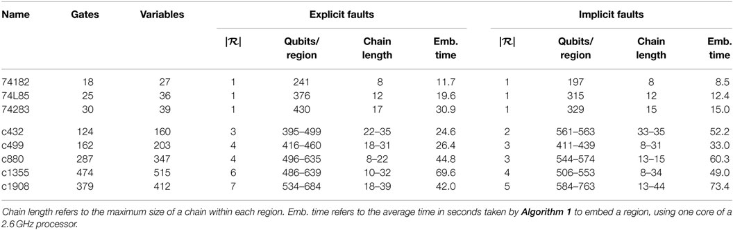
Table 1. Statistics for the 74X Series and ISCAS ‘85 benchmarks as embedded on a D-Wave 2X processor, including number of regions | ℛ| in the decomposition.

3.2. Generating Diverse Solutions

To test the D-Wave hardware’s ability to generate diverse solutions, we consider the problem of finding all min-cardinality fault diagnoses for a given observation. This is computationally not only more difficult than finding a single diagnosis but also more realistic from the perspective of applications. Again, state-of-the-art performance in the weak fault model is achieved using a SAT-solver (Metodi et al., 2014).

The hardware’s natural ability to rapidly generate low-energy samples lends itself to applications in which a diverse set of optimal solutions are required. Unfortunately, samples taken from the D-Wave hardware do not conform to a Boltzmann distribution, owing to both noise and quantum mechanical effects. In contrast with greedy stochastic search (Feldman et al., 2007), min-cardinality solutions will not generally be sampled with equal probability. In practice, Gibbs sampling (Geman and Geman, 1984) and other post-processing techniques may be used to make a distribution of ground states more uniform.

We restricted to the 74X-Series circuits in Table 1, which can be entirely embedded within the current hardware architecture. For each input–output pair for a circuit, we used SharpSAT (Thurley, 2006) to enumerate the min-cardinality diagnosis set Ω^≤ and then drew 1000|Ω^≤| samples from the QA hardware. Ising models were pre-processed with roof-duality (Boros and Hammer, 2002) and arc-consistency (Mackworth, 1977), allowing certain variables to be fixed in polynomial time. Random spin–reversal transformations (“gauge transformations”) were applied to mitigate the effects of intrinsic control error in the D-Wave hardware. Samples were post-processed using majority vote to repair broken chains, followed by greedy bit-flipping in the original constraint satisfaction space to descend to local minima. See King and McGeoch (2014) for more details on pre- and post-processing.

The results in Figure 3 show the expected number of samples needed to see all min-fault diagnoses at least once, together with the number of samples needed to see just a single min-fault diagnosis. Namely, if p_i denotes the fraction of all samples taken that correspond to min-fault diagnosis i, then the expected number of samples required to find a single min-fault solution is $1∕{\sum }_i{p}_i$, and the expected number of samples required to find all min-fault solutions is ${\mathit{\int }}_0^{\infty }\left(1-{\prod }_i\left(1-e^{-p_{i}t}\right)\right)\mathrm{dt}$. [This is the coupon collecting problem with non-uniform probabilities (Von Schelling, 1954; Flajolet et al., 1992).] Following Feldman et al. (2007), we also computed the expected fraction of all min-fault diagnoses found when taking N|Ω^≤| samples, for N ∈ {10, 100, 1000}. These results are summarized in Table 2.

FIGURE 3

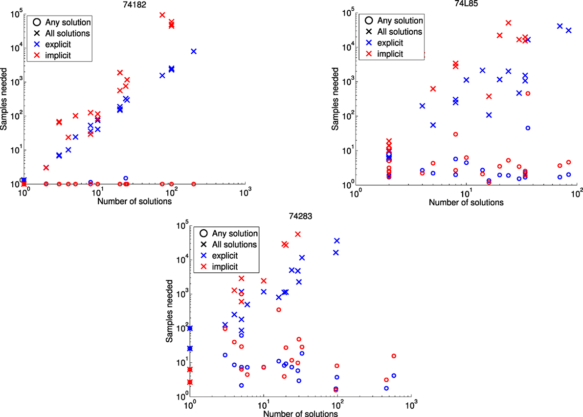
Figure 3. Performance in finding all min-fault diagnoses for the 74X benchmarks using a D-Wave 2X processor. Missing ×’s indicate that not all solutions were found.

TABLE 2

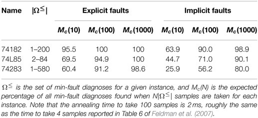
Table 2. Performance in finding all min-fault diagnoses for the 74X benchmarks using a D-Wave 2X processor.

3.3. Solving Large Problems

We tested the performance of the D-Wave hardware in solving the fault diagnosis problem for circuits too large to be embedded. On the regions produced in §3.1, we applied two algorithms: dual decomposition (DD) from Bian et al. (2014) and divide-and-concur (DC) from §2.5. These two algorithms were chosen because they lead to relatively high success rates in software simulations, without the complications of finite-temperature sampling (as in Algorithm 2) or multiple hardware calls for each region within each iteration [as in the belief propagation of Bian et al. (2014)].

To measure algorithm performance independent of quantum annealing, we also found the minima for regional Ising models exactly using low-treewidth variable elimination (Koller and Friedman, 2009). Such an exact solver (SW) gives an upper bound on the performance of a decomposition algorithm.

In Figure 4A, we show the number of successful min-fault diagnoses out of 20 instances for several of the ISCAS ‘85 benchmark circuits. Using the exact solver, we attempted to solve each fault diagnosis instance 100 times, and recorded the median number of successes across the 20 instances for each circuit. Using the D-Wave hardware, we attempted to solve each instance once. A summary of the D-Wave hardware performance on each regional optimization problem is given in Figure 4B. Each problem was solved by drawing 20,000 samples across 20 spin-reversal transformations, with pre- and post-processing as in §3.2.

FIGURE 4

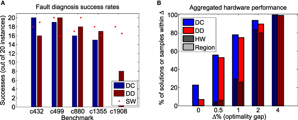
Figure 4. (A) Summary of D-Wave hardware success rate using divide-and-concur (DC) and dual decomposition (DD), compared with the same decomposition algorithm using an exact low-treewidth software solver (SW). (B) Percentage of hardware samples (HW) and regional solutions (Region) within Δ% of optimality across all instances tested.

Note that the overall performance of the decomposition algorithms using D-Wave’s heuristic optimizer is similar to that using an exact solver, despite the fact that the D-Wave hardware does not solve every sub-problem to optimality. This suggests that QA hardware that provides only approximate solutions in the form of low-energy samples can still be used to solve large optimization problems provided it can capture a sufficiently non-trivial portion of the original problem.

4. Discussion

In this paper, we have expanded on the approach given in Bian et al. (2014) to solve large discrete optimization problems using quantum annealing hardware limited by issues of precision, connectivity and size. This approach is based on two ideas: locally structured embeddings, in which hardware precision is mitigated by mapping constraints of a CSP onto disjoint subgraphs of a hardware graph, at the cost of additional qubits; and decomposition algorithms, in which large problems are solved by passing messages between smaller, embeddable regions. We demonstrate that for some problems the qubit cost of locally structured embeddings is offset by improved hardware performance, and we propose both new embedding techniques and new decomposition algorithms.

Applying these techniques with the D-Wave 2X device, we are able to solve non-trivial problems in model-based fault diagnosis. For small, directly embeddable circuits, sampling from the D-Wave hardware allows us to find all min-fault diagnoses across a range of test observations, despite not sampling those diagnoses uniformly. For larger circuits, decomposition algorithms with up to 5 regions prove successful in identifying a single min-fault diagnosis. While the total running times of the decomposition algorithms are not currently competitive with the fastest classical techniques, both the speed and the performance of the algorithms improve dramatically with the size of the quantum hardware available.

Two of the most important directions for future research are as follows:

1. Expanding penalty-modeling techniques to more qubits. As the available hardware grows larger, large energy gaps, and other forms of error correction will become more important to finding the ground state in quantum annealing. In addition, a better understanding of the performance trade-off between larger energy gap and fewer qubits is needed.

2. Alternate strategies for decomposition algorithms. Since minor embedding is itself a difficult discrete optimization problem, current decomposition algorithms are hampered by the need for fixed regions with pre-computed embeddings. More research is needed into circumventing the need for fixed regions, combining quantum annealing with the best classical constraint satisfaction methods, and making better use of the fast sampling capabilities of the available hardware.

Author Contributions

All authors contributed to the research and writing of this manuscript.

Conflict of Interest Statement

The authors declare that the research was conducted in the absence of any commercial or financial relationships that could be construed as a potential conflict of interest.

Footnotes

1. ^To see this, note that [h, J_P] is a collection of penalty models for constraints on independent variables, each of which achieves its ground state energy when the constraint is satisfied, while [0, J_C] achieves its ground state energy whenever no chains are broken.
2. ^More generally, weighted CSP can be solved by weighting reified variables representing constraints.
3. ^Lackey, B. (in preparation). A belief propagation algorithm based on regional decomposition.
4. ^e.g., http://dx15.sciencesconf.org/
5. ^http://web.eecs.umich.edu/∼jhayes/iscas.restore/benchmark.html

References

Amin, M. H. (2015). Searching for quantum speedup in quasistatic quantum annealers. Phys. Rev. A 92, 052323. doi: 10.1103/PhysRevA.92.052323

CrossRef Full Text | Google Scholar

Benedetti, M., Realpe-Gómez, J., Biswas, R., and Perdomo-Ortiz, A. (2015). Estimation of effective temperatures in a quantum annealer and its impact in sampling applications: a case study towards deep learning applications. arXiv:1510.07611.

Google Scholar

Berkley, A. J., Johnson, M. W., Bunyk, P., Harris, R., Johansson, J., Lanting, T., et al. (2010). A scalable readout system for a superconducting adiabatic quantum optimization system. Supercond. Sci. Tech. 23, 105014. doi:10.1088/0953-2048/23/10/105014

CrossRef Full Text | Google Scholar

Bian, Z., Chudak, F., Israel, R., Lackey, B., Macready, W. G., and Roy, A. (2014). Discrete optimization using quantum annealing on sparse Ising models. Front. Phys. 2:56. doi:10.3389/fphy.2014.00056

CrossRef Full Text | Google Scholar

Bian, Z., Chudak, F., Macready, W. G., Clark, L., and Gaitan, F. (2013). Experimental determination of Ramsey numbers. Phys. Rev. Lett. 111, 130505. doi:10.1103/PhysRevLett.111.130505

PubMed Abstract | CrossRef Full Text | Google Scholar

Boros, E., and Hammer, P. L. (2002). Pseudo-Boolean optimization. Discrete Appl. Math. 123, 155–225. doi:10.1016/S0166-218X(01)00341-9

CrossRef Full Text | Google Scholar

Bunyk, P., Hoskinson, E., Johnson, M., Tolkacheva, E., Altomare, F., Berkley, A., et al. (2014). Architectural considerations in the design of a superconducting quantum annealing processor. IEEE Trans. Appl. Supercond. 24, 1–10. doi:10.1109/TASC.2014.2318294

CrossRef Full Text | Google Scholar

Cai, J., Macready, W. G., and Roy, A. (2014). A practical heuristic for finding graph minors. arXiv:1406.2741.

Google Scholar

Chan, T., Cong, J., Kong, T., and Shinnerl, J. (2000). “Multilevel optimization for large-scale circuit placement,” in IEEE/ACM International Conference on Computer Aided Design, 2000. ICCAD-2000 (San Jose, CA: IEEE), 171–176.

Google Scholar

Chopra, S., Gorres, E. R., and Rao, M. R. (1992). Solving the Steiner tree problem on a graph using branch and cut. INFORMS J. Comput. 4, 320–335. doi:10.1287/ijoc.4.3.320

CrossRef Full Text | Google Scholar

Dickson, N. G., Johnson, M. W., Amin, M. H., Harris, R., Altomare, F., Berkley, A. J., et al. (2013). Thermally assisted quantum annealing of a 16-qubit problem. Nat. Commun. 4, 1903. doi:10.1038/ncomms2920

PubMed Abstract | CrossRef Full Text | Google Scholar

Douglass, A., King, A. D., and Raymond, J. (2015). “Constructing SAT filters with a quantum annealer,” in Theory and Applications of Satisfiability Testing – SAT 2015, Volume 9340 of Lecture Notes in Computer Science, eds M. Heule and S. Weaver (Cham: Springer), 104–120.

Google Scholar

Farhi, E., Goldstone, J., Gutmann, S., and Sipser, M. (2000). Quantum computation by adiabatic evolution. arXiv:quant-ph/0001106.

Google Scholar

Feldman, A., Provan, G., and van Gemund, A. (2007). “Approximate model-based diagnosis using greedy stochastic search,” in Abstraction, Reformulation, and Approximation, Volume 4612 of Lecture Notes in Computer Science, eds I. Miguel and W. Ruml (Berlin: Springer), 139–154.

Google Scholar

Finilla, A. B., Gomez, M. A., Sebenik, C., and Doll, D. J. (1994). Quantum annealing: a new method for minimizing multidimensional functions. Chem. Phys. Lett. 219, 343–348.

Google Scholar

Flajolet, P., Gardy, D., and Thimonier, L. (1992). Birthday paradox, coupon collectors, caching algorithms and self-organizing search. Discrete Appl. Math. 39, 207–229. doi:10.1016/0166-218X(92)90177-C

CrossRef Full Text | Google Scholar

Geman, S., and Geman, D. (1984). Stochastic relaxation, Gibbs distributions, and the Bayesian restoration of images. IEEE Trans. Pattern Anal. Mach. Intell. PAMI-6, 721–741. doi:10.1109/TPAMI.1984.4767596

PubMed Abstract | CrossRef Full Text | Google Scholar

Gester, M., Müller, D., Nieberg, T., Panten, C., Schulte, C., and Vygen, J. (2013). BonnRoute: algorithms and data structures for fast and good VLSI routing. ACM Trans. Des. Autom. Electron. Syst. 18, 32:1–32:24. doi:10.1145/2442087.2442103

CrossRef Full Text | Google Scholar

Gravel, S., and Elser, V. (2008). Divide and concur: a general approach to constraint satisfaction. Phys. Rev. E Stat. Nonlin. Soft Matter Phys. 78, 036706. doi:10.1103/PhysRevE.78.036706

PubMed Abstract | CrossRef Full Text | Google Scholar

Hansen, M., Yalcin, H., and Hayes, J. (1999). Unveiling the ISCAS-85 benchmarks: a case study in reverse engineering. IEEE Design Test Comput. 16, 72–80. doi:10.1109/54.785838

CrossRef Full Text | Google Scholar

Harris, R., Johansson, J., Berkley, A. J., Johnson, M. W., Lanting, T., Han, S., et al. (2010). Experimental demonstration of a robust and scalable flux qubit. Phys. Rev. B 81, 134510. doi:10.1103/PhysRevB.81.134510

CrossRef Full Text | Google Scholar

Jia, H., Moore, C., and Selman, B. (2005). “From spin glasses to hard satisfiable formulas,” in Theory and Applications of Satisfiability Testing, Volume 3542 of Lecture Notes in Computer Science, eds H. H. Hoos and D. G. Mitchell (Berlin, Heidelberg: Springer), 199–210.

Google Scholar

Johnson, M. W., Amin, M. H. S., Gildert, S., Lanting, T., Hamze, F., Dickson, N., et al. (2011). Quantum annealing with manufactured spins. Nature 473, 194–198. doi:10.1038/nature10012

PubMed Abstract | CrossRef Full Text | Google Scholar

Kadowaki, T., and Nishimori, H. (1998). Quantum annealing in the transverse Ising model. Phys. Rev. E 58, 5355. doi:10.1103/PhysRevE.58.5355

CrossRef Full Text | Google Scholar

Kahng, A. B., Lienig, J., Markov, I. L., and Hu, J. (2011). VLSI Physical Design – From Graph Partitioning to Timing Closure. Dordrecht: Springer.

Google Scholar

Karypis, G., and Kumar, V. (1998). A fast and high quality multilevel scheme for partitioning irregular graphs. SIAM J. Sci. Comput. 20, 359–392. doi:10.1137/S1064827595287997

CrossRef Full Text | Google Scholar

King, A. D., and McGeoch, C. C. (2014). Algorithm engineering for a quantum annealing platform. arXiv:1410.2628.

Google Scholar

Koller, D., and Friedman, N. (2009). Probabilistic Graphical Models – Principles and Techniques. MIT Press.

Google Scholar

Kou, L. T., Markowsky, G., and Berman, L. (1981). A fast algorithm for Steiner trees. Acta Inform. 15, 141–145. doi:10.1007/BF00288961

CrossRef Full Text | Google Scholar

Kurtoglu, T., Narasimhan, S., Poll, S., Garcia, D., Kuhn, L., de Kleer, J., et al. (2009). First international diagnosis competition-DXC09. Proc. DX09 383–396.

Google Scholar

Mackworth, A. K. (1977). Consistency in networks of relations. Artif. Intell. 8, 99–118. doi:10.1016/0004-3702(77)90007-8

CrossRef Full Text | Google Scholar

McKay, B. D. (1998). Isomorph-free exhaustive generation. J. Algorithm. 26, 306–324. doi:10.1006/jagm.1997.0898

CrossRef Full Text | Google Scholar

Metodi, A., Stern, R., Kalech, M., and Codish, M. (2014). A novel SAT-based approach to model based diagnosis. J. Artif. Intell. Res. 51, 377–411. doi:10.1613/jair.4503

CrossRef Full Text | Google Scholar

Narodytska, N., and Bacchus, F. (2014). “Maximum satisfiability using core-guided MaxSAT resolution,” in Proceedings of the Twenty-Eighth AAAI Conference on Artificial Intelligence (Québec City, QC: AAAI Press), 2717–2723.

Google Scholar

Perdomo-Ortiz, A., Fluegemann, J., Narasimhan, S., Biswas, R., and Smelyanskiy, V. (2015). A quantum annealing approach for fault detection and diagnosis of graph-based systems. Eur. Phys. J. Spec. Top. 224, 131–148. doi:10.1140/epjst/e2015-02347-y

CrossRef Full Text | Google Scholar

Poll, S., de Kleer, J., Abreau, R., Daigle, M., Feldman, A., Garcia, D., et al. (2011). “Third international diagnostics competition-DXC 11,” in Proc. of the 22nd International Workshop on Principles of Diagnosis, 267–278.

Google Scholar

Rajagopalan, S., and Vazirani, V. (1999). “On the bidirected cut relaxation for the metric Steiner tree problem (extended abstract),” in Proceedings of the 10th Annual ACM-SIAM Symposium on Discrete Algorithms (Philadelphia, PA: SIAM), 742–751.

Google Scholar

Raymond, J., Yarkoni, S., and Andriyash, E. (2016). Global warming: Temperature estimation in annealers. arXiv:1606.00919.

Google Scholar

Rieffel, E. G., Venturelli, D., O’Gorman, B., Do, M. B., Prystay, E. M., and Smelyanskiy, V. N. (2015). A case study in programming a quantum annealer for hard operational planning problems. Quantum Inf. Process. 14, 1–36. doi:10.1007/s11128-014-0892-x

CrossRef Full Text | Google Scholar

Rönnow, T. F., Wang, Z., Job, J., Boixo, S., Isakov, S. V., Wecker, D., et al. (2014). Defining and detecting quantum speedup. Science 345, 420–424. doi:10.1126/science.1252319

CrossRef Full Text | Google Scholar

Roy, J. A., Papa, D. A., Adya, S. N., Chan, H. H., Ng, A. N., Lu, J. F., et al. (2005). “Capo: robust and scalable open-source min-cut floorplacer,” in ISPD (New York, NY: ACM), 224–226.

Google Scholar

Siddiqi, S., and Huang, J. (2007). “Hierarchical diagnosis of multiple faults,” in Proceedings of the 20th International Joint Conference on Artificial Intelligence (IJCAI) (San Francisco, CA: Morgan Kaufmann Publishers Inc.), 581–586.

Google Scholar

Stern, R., Kalech, M., and Elimelech, O. (2014). “Hierarchical diagnosis in strong fault models,” in Twenty Fifth International Workshop on Principles of Diagnosis (Graz, Austria).

Google Scholar

Tan, P.-N., Steinbach, M., and Kumar, V. (2005). Introduction to Data Mining, (First Edition). Boston, MA: Addison-Wesley.

Google Scholar

Thurley, M. (2006). “sharpSAT – counting models with advanced component caching and implicit BCP,” in SAT, Volume 4121 of Lecture Notes in Computer Science, eds A. Biere and C. P. Gomes (Berlin: Springer), 424–429.

Google Scholar

Venturelli, D., Mandrà, S., Knysh, S., O’Gorman, B., Biswas, R., and Smelyanskiy, V. (2015a). Quantum optimization of fully connected spin glasses. Phys. Rev. X 5, 031040. doi:10.1103/PhysRevX.5.031040

CrossRef Full Text | Google Scholar

Venturelli, D., Marchand, D. J. J., and Rojo, G. (2015b). Quantum annealing implementation of job-shop scheduling. arXiv:1506.08479.

Google Scholar

Von Schelling, H. (1954). Coupon collecting for unequal probabilities. Am. Math. Mon. 61, 306–311. doi:10.2307/2307466

CrossRef Full Text | Google Scholar

Yedidia, J. S. (2011). Message-passing algorithms for inference and optimization. J. Stat. Phys. 145, 860–890. doi:10.1007/s10955-011-0384-7

CrossRef Full Text | Google Scholar

Yedidia, J. S., Freeman, W. T., and Weiss, Y. (2005). Constructing free-energy approximations and generalized belief propagation algorithms. IEEE Trans. Inf. Theory 51, 2282–2312. doi:10.1109/TIT.2005.850085

CrossRef Full Text | Google Scholar

Zick, K. M., Shehab, O., and French, M. (2015). Experimental quantum annealing: case study involving the graph isomorphism problem. Sci. Rep. 5, 11168. doi:10.1038/srep11168

PubMed Abstract | CrossRef Full Text | Google Scholar