A Model of Fast Hebbian Spike Latency Normalization

1. Introduction

Since the discovery of long-term synaptic plasticity by Bliss and Lømo (1973), Hebb's postulate that “cells that fire together wire together” (Hebb, 1949; Schatz, 1992) has become the prominent hypothesis whereby the brain learns and forms new memories. Generally speaking, Hebbian learning may refer to any change of efficacy of synaptic transmission (i.e., the “synaptic weight”) by synaptic plasticity that solely depends on correlations between firing activities of pre- and postsynaptic neurons (Abbott and Nelson, 2000). In this regard, spike-timing–dependent plasticity (STDP) may be considered the experimental hallmark of Hebbian learning, insofar as it allows a synapse to be potentiated by correlated pre/post spike pairs while being depressed by correlated post/pre spike pair (Markram et al., 1997; Bi and Poo, 1998).

Despite being appealing for its simple formulation, Hebbian plasticity, and thus STDP, are prone to instability. Depressed synapses tend to become further depressed, and vice-versa, potentiated synapses tend to grow even stronger (Sjöström et al., 2008). Ad-hoc mechanisms that compensate for such instabilities are hypothesized to coexist with Hebbian plasticity. Collectively, these mechanisms are known as homeostatic plasticity and are experimentally known to prevent runaway of excitation of single neurons, thereby maintaining a stable level of firing activity (Turrigiano, 2008).

Homeostatic plasticity results in compensatory changes in the overall synaptic drive (e.g., synaptic scaling Turrigiano et al., 1998), changes in the neuronal excitability (intrinsic plasticity Desai, 2003) or changes to the plasticity rules themselves by metaplasticity (Abraham and Bear, 1996; Abraham, 2008). All these experimentally-found homeostatic mechanisms have a relatively slow response compared to rapid plasticity, which is thought necessary for learning. While synaptic weights can change on the timescale of seconds to minutes (Markram et al., 1997; Bi and Poo, 1998; Sjöström et al., 2008), noticeable changes caused by homeostasis generally take hours or even days (Turrigiano et al., 1998; Turrigiano, 1999; Turrigiano and Nelson, 2004; Watt and Desai, 2010). As a consequence, it has been conjectured that a further, fast form of homeostatic plasticity, acting on time scales comparable to those of learning, must exist to maintain firing stability (Zenke et al., 2013; Yger and Gilson, 2015) although its biophysical correlates remain to be explored.

Here we address this conundrum by exploring the requirements for stability of Hebbian learning in the context of rhythmic activity which alternates between high and low rate periods. We refer to these periods as UP and DOWN phases. In this regard, we show by analytical arguments and numerical simulations that stability of activity and weight normalization can be an emergent property of Hebbian plasticity through postsynaptic spike latency normalization (SLN) with respect to the onset of an UP phase of activity. We introduce a Hebbian STDP-based metaplasticity rule, which we refer to as the SLN rule, that includes online estimation of the total synaptic input per neuron by making use of the transitions between UP and DOWN phases. These phases can either be compared to the scenario, ubiquitous in the brain (Gray and McCormick, 1996; Lesica and Stanley, 2004; Engel et al., 2016), of activity that varies strongly and abruptly over time or to long UP and DOWN phases that occur during sleep (Steriade et al., 2001). The effect of sleep on plasticity and homeostasis is not completely established. However, the synaptic homeostasis hypothesis (SHY) considers that synaptic potentation resulting from increased neuronal and synaptic activity by sensory stimulation during wakefulness (Vyazovskiy et al., 2008; Liu et al., 2010; Bushey et al., 2011; Maret et al., 2011) must be downscaled during sleep to re-equilibrate the brain's energy demand, but the homeostatic mechanism for such rescaling is not understood (Tononi and Cirelli, 2003, 2006, 2014). Remarkably, the SLN rule results in fast weight normalization for short UP and DOWN phases which makes it a candidate for a fast homeostasis mechanism during periods of wakefulness whereas, for long UP phases, it results in rescaling of the weights at a lower level in agreement with SHY. We discuss the biophysical correlates and advantages of this rule with respect to other models.

2. Materials and Methods

2.1. Neuronal models

We study two models which differ at their level of abstraction and we characterize them by the type of neurons which are specific to each model. We consider integrate and fire neurons either without (SIF) or with leak (LIF). Hence, to distinguish the models, we refer to them as “the model without leak” or “the model with leak.” When describing the models we adopt the convention to first describe aspects which are common to both models along with minor differences. We present then details pertaining to the model without leak followed by those of the model with leak. In both models, a neuron fires an action potential when its membrane potential υ(t) reaches a threshold θ_υ, after which it is reset to V_r, and held to this reset potential for a refractory period τ_ref. The subthreshold dynamics of υ(t) thus evolves according to:

$\begin{array}{ll}{C}_m\frac{d}{dt}\upsilon =g\left(\upsilon \right)+I_{\text{syn}},& (1)\end{array}$

where g(υ) is a voltage dependent term and I_syn is a term which captures synaptic input. Most results concern binary synapses and therefore we differentiate between weak (w) and strong (s) synapses whose weights we respectively denote by w_w and w_s.

2.1.1. Model without Leak

In Equation (1) we set g(υ) = 0 and the input current is the sum of current-based synaptic inputs. A spike of neuron j in the input population I at time t_j arrives at the postsynaptic neuron without delay and is modeled by a Dirac delta scaled by the synaptic weight w_j, i.e., $I_{\text{syn}}=\sum _{j\in I}\sum _{t_j}{w}_j·\delta (t-t_j)$ (see Figure 1Aa).

FIGURE 1

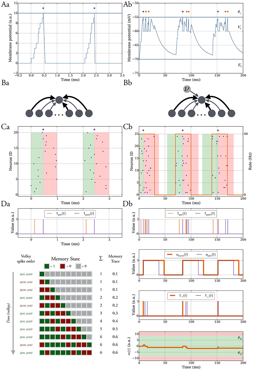
Figure 1. The model without leak (left column) vs. the model with leak (right column). (A) In both models the neurons spike when their membrane potential reaches a threshold θ_v after which it is reset to a value V_r and held at that value for τ_ref ms. In the model without leak (a), the neuron receives current-based input whereas in the model with leak (b), the input is conductance-based and the membrane potential decays exponentially. The spikes are shown as stars. We refer to the purple spikes as “distinguished” spikes (DSPs). They block other postsynaptic spikes from receiving that label for a period of T_burst ms. (B) Network models. A single target neuron that receives input from a population (a). In the model with leak (b), the neuron additionally receives constant noise input with weight w_n at rate ν. The synapses are binary and can be either weak (light gray), with weight w_w, or strong, with weight w_s (dark gray). (C) Input spike model. (a) Each input neuron spikes once at a time chosen uniformly at random within a short interval. Presynaptic spikes which occur before (after) the postsynaptic spike lead to a potentiation (depression) signal which is highlighted with a green (red) shaded region. (b) The input spikes are modeled as an inhomogeneous Poisson process. The input neurons switch between a high rate UP phase and a low rate DOWN phase (orange curve with respect to right y-axis). The presynaptic spikes which occur in a window before (after) the distinguished postsynaptic spike trigger potentiation (depression) signals and the window is highlighted in green (red). (D) Learning rule. Each synapse has a memory trace m(t) that is modified for certain spike pair events, similar to standard STDP. (a) Potentiation and depression signals are always with respect to spike pairs and we track the spikes with the variables 𝟙_pre and 𝟙_post. The memory in the model without leak contains the last M potentiation and depression signals and the memory trace is the fraction of potentiation signals. (b) Variables to define distinguished spikes (DSPs), potentiation and depression signals, and the memory trace m(t) (see Section 2.3 for details).

We consider both deterministic and probabilistic synapses (Branco and Staras, 2009) for which a transmission probability p_r < 1 is tantamount to multiplying presynaptic spikes by the outcome of a Bernoulli trial with probability p_r.

2.1.2. Model with Leak

In Equation (1) the leak is captured by the term g(υ) = −g_L(υ − E_L) and I_syn is the sum of conductance-based synaptic inputs. The inputs decay exponentially with time constant τ_syn and have a reversal potential E_e, that is I_syn = g_e(t) · (V(t) − E_e) where:

$\begin{array}{ll}{\tau }_{\text{syn}}\frac{d}{dt}{g}_e=-g_e\left(t\right)+{\displaystyle \sum _{j\in I}}{\displaystyle \sum _{t_j}}{w}_j·\delta \left(t-t_j-t_{\text{delay}}\right).& (2)\end{array}$

The sum $\sum _{t_j}\delta (t-t_j-t_{\text{delay}})$ corresponds to presynaptic spikes of neuron j ∈ I, each occurring at time t_j and contributing to postsynaptic depolarization in an amount of w_j after a delay t_delay (see Figure 1Ab).

2.2. Synaptic Input Configuration

We consider the scenario of a single neuron which receives d independent synaptic inputs, each associated with a presynaptic neuron (Figure 1Ba). In the model with leak, we model background activity by stimulating the postsynaptic neuron by an external Poisson synaptic current of strength w_n at rate ν (Hô and Destexhe, 2000) (Figure 1Bb).

2.2.1. Model without Leak

We assume that presynaptic neurons fire together in short pulses, hereafter termed as “volleys” (Figure 1Ca). In particular, the postsynaptic neuron potential is at rest (i.e., 0) at the start of a volley, and for a volley of duration T_U, at time t, each presynaptic neuron independently selects a spike uniformly at random in the interval [t, t + T_U]. The time between two consecutive volleys is T_D ms. Most of our analysis is carried out under the random order assumption that volley spikes are uniformly distributed, although we also consider deviations from this assumption in Section 3.1.2.

2.2.2. Model with Leak

Each presynaptic neuron fires according to an inhomogeneous Poisson process (unless differently specified). The rate of the process alternates between DOWN phases of low rate values (λ_D) and UP phases of high rate values (λ_U). The duration of each DOWN and UP phase corresponds to the parameters T_D and T_U, respectively (Figure 1Cb). The volleys in the model without leak may be regarded as the limiting case of short UP phases and they lead to analytical tractability of the model. In one setting when we study robustness against input parameter variations we shift the input rate function of each input neuron by some random delay, independently drawn from a uniform distribution in [0, σ].

2.3. Learning Rule

2.3.1. Memory Trace

Each synapse tracks pre- and postsynaptic spikes by means of a scalar memory trace m(t) which is updated similarly to classical STDP (Morrison et al., 2008). Accordingly, presynaptic spikes that happen in a short interval T_early before a postsynaptic spike, all increase m(t) promoting synaptic potentiation. Conversely, presynaptic spikes following a postsynaptic spike in a time window T_late, decrease m(t) which can lead to synaptic depression (see green and red shaded regions in Figure 1C). We refer to these spike pair events as potentiation and depression signals and we denote them by the binary indicator variables 𝟙_↑(t) and, respectively, 𝟙_↓(t).

2.3.2. Model without Leak

For volley input, these signals simply correspond to the spike order of a synapse in each volley, that is 𝟙_↑(t) is 1 at the time of a postsynaptic spike if it was preceded by a presynaptic spike in that volley and similarly 𝟙_↓(t) is 1 at the time of a presynaptic spike if it was preceded by a postsynaptic spike in that volley.

The memory trace in this setting is given by the moving average of learning signals which are potentiation signals (see Figure 1Da), that is, let S^(signals)(M) be a set containing the time of the last M learning signals, then

$\begin{array}{ll}m\left(t\right)\equiv M^{-1}{\displaystyle \sum _{t^{\prime }\in S^{\text{(signals)}}\left(M\right)}}{\mathrm{𝟙}}_{\uparrow }\left(t^{\prime }\right).& (3)\end{array}$

2.3.3. Model with Leak

The main difference in this setting is that the neurons can spike more than once in an UP phase instead of at most once in a volley. The memory trace is updated for spikes pairs corresponding to potentiation and depression signals as in the model without leak. However, we restrict the pairs which trigger such signals to those which involve the first postsynaptic spike in an UP phase (purple stars in Figure 1). We will hereafter dub such postsynaptic spikes as distinguished spikes (DSPs). This restriction accounts for the fact that STDP may involve more complex interactions between pre- and postsynaptic firing rather than those considered in classic doublet STDP models (Pfister and Gerstner, 2006). To define the memory trace and its update rules formally we therefore first define all relevant variables (for an overview, see Figure 1Db).

For a synapse, we denote by 𝟙_pre(t) and 𝟙_post(t) the indicator variables which are 1 at time t if the corresponding pre- or postsynaptic neuron spiked and 0 otherwise. We use these variables to derive indicator variables for potentiation and depression signals, however, for the derivation, we also require variables which monitor whether a DSP recently occurred and whether presynaptic spikes occur in a time window around it. In this regard, we introduce the binary variable o_burst(t) which is 1 if a DSP occurred in [t − T_burst, t), and 0 otherwise. We define it recursively as follows:

$\begin{array}{ll}{o}_{\text{burst}}\left(t\right)={\displaystyle \sum _{t^{\prime }\in S^{\text{post}}\left(t-T_{\text{burst}},t\right)}}(1-o_{\text{burst}}(t^{\prime }))& (4)\end{array}$

where $S^{\text{post}}(t_1,t_2)$ denotes the set of all postsynaptic spikes in the interval [t₁, t₂). Similarly, we monitor the depression signal window by the binary variable o_late(t) which is 1 in a time window T_late after a DSP and 0 otherwise, i.e.,

$\begin{array}{ll}{o}_{\text{late}}\left(t\right)={\displaystyle \sum _{t^{\prime }\in S^{\text{post}}(t-T_{\text{late}},t)}}(1-o_{\text{burst}}(t^{\prime })).& (5)\end{array}$

Accordingly, the depression and potentiation signal indicator variables are given by

$\begin{array}{l}{\mathrm{𝟙}}_{\downarrow }\left(t\right)={\mathrm{𝟙}}_{\text{pre}}\left(t\right)·o_{\text{late}}\left(t\right),\\ {\mathrm{𝟙}}_{\uparrow }\left(t\right)={\mathrm{𝟙}}_{\text{post}}\left(t\right)·\left(1-o_{\text{burst}}\left(t\right)\right)·min\left\{1,|S^{\text{pre}}\left(t-T_{\text{early}},t\right)|\right\}& (6)\end{array}$

where $S^{\text{pre}}(t_1,t_2)$ denotes the set of all presynaptic spikes in the interval [t₁, t₂).

Whenever 𝟙_↓(t) is 1 we update the memory trace m(t) as follows

$\begin{array}{ll}m\left(t\right)\leftarrow -1+\gamma m\left(t\right)& (7)\end{array}$

where γ defines the attenuation of the pre-existing memory trace. Similarly, whenever 𝟙_↑(t) is 1 we apply

$\begin{array}{ll}m\left(t\right)\leftarrow 1+\gamma m\left(t\right)& (8)\end{array}$

for each presynaptic spike in the interval [t − T_early, t), i.e., we apply the update $\left|S^{\text{pre}}(t_{\text{post}}-T_{\text{early}},t_{\text{post}})\right|$ times.

2.3.4. Weight Update

The plasticity of the synapse depends on the value of m(t). In both the model with and without leak, the update of the synaptic weight is applied similarly. The main difference is that in the model without leak the weight update rule is applied only after every L-th update to the memory trace (L ≥ M) whereas for the model with leak the weight update follows every memory trace update. In a weight update, the weight can change if and only if m(t) > θ_P or m(t) < θ_D, where θ_P and θ_D are the depression and potentiation thresholds (the interval [θ_D, θ_P] is shown as a shaded green region in Figure 1Db). Formally, the change in synaptic weight is probabilistic, which has been considered before (Standage and Trappenberg, 2006), and, in particular, is subjected to the outcome of a Bernoulli trial with probability p_s→w for depression and p_w→s for potentiation. This approach is necessary to prevent many synapses from changing their weight together with the risk of destabilizing postsynaptic firing (see Section 3.2.1). The weight update rule is given as follows

$\begin{array}{cc}w(t)\leftarrow w(t)+\{\begin{array}{ll}{\Delta }_{d}w(t)\hfill & \text{with probability }{p}_{s\to w}\text{ if }m(t)<{\theta }_D,\hfill \\ {\Delta }_{p}w(t)\hfill & \text{with probability }{p}_{w\to s}\text{ if }m(t)>{\theta }_P,\hfill \\ 0\hfill & \text{otherwise}.\hfill \end{array}& (9)\end{array}$

With binary synapses, which have weights w_s and w_w, the weight changes according to:

$\begin{array}{l}{\Delta }_{p}w(t)=\{\begin{array}{ll}{w}_s-w_w\hfill & \text{if }w(t)=w_w,\hfill \\ 0\hfill & \text{otherwise}.\hfill \end{array}\\ {\Delta }_{d}w(t)=\{\begin{array}{ll}{w}_w-w_s\hfill & \text{if }w(t)=w_s,\hfill \\ 0\hfill & \text{otherwise}.\hfill \end{array}& (10)\end{array}$

2.4. Spike Latency Normalization

In the model with leak, we achieve homeostatic plasticity by normalization of the mean timing of the first postsynaptic spike (that is, the DSP) with respect to an UP phase. In this regard it may be noted that for a given input rate function, the distribution of inter-spike intervals f(t) of a neuron receiving d_s strong synaptic inputs out of d inputs in total is known (Burkitt, 2006a,b), and so is the mean first passage time (Cox and Miller, 1977; Ricciardi, 1977; Tuckwell, 1988). Accordingly, denoting by t_DSP the relative time of the first postsynaptic spike in an UP phase, and keeping in mind that f(t) is defined for t ∈ [0, T_U], the expected first passage time, that is the average relative timing of DSP with respect to the onset of an UP phase is:

$t_{\text{DSP}}\equiv 𝔼[t_{\text{first}}|t_{\text{first}}<T_U]={\displaystyle {\int }_{t=0}^{T_U}t}·f(t)dt.(11)$

For convenience we define $r\equiv \frac{t_{\text{DSP}}}{T_U}$ to be the expected time of the first spike within an UP phase relative to the length of the UP phase. It may then be noted that setting the duration of a DSP (i.e., T_burst) such that T_burst ≥ T_U, ensures that only one DSP occurs in an UP phase. In this fashion, it is possible to distinguish between early vs. late presynaptic spikes, that is input spikes arriving T_early before and T_late after the DSP as required by our learning rule (6). Furthermore, choosing T_early, T_late ≥ T_U enables the contribution of all presynaptic spikes to potentiation/depression in an UP phase (for results related to a large value of T_U see Section 3.2.2). In this fashion, for UP phases sufficiently apart from each other, so as to neglect synaptic changes due to overlapping learning signals from consecutive UP phases, our learning rule performs normalization of the expected spike latency t_DSP. The details of how this is possible are reported in Sections 3.1.1, 3.1.2, and 3.2.1.

2.5. Heterogeneous (Multimodal) Synaptic Weights

Besides binary synapses, we also consider multimodal synapses for the model without leak in Section 3.2.3, that is synapses whose weight can assume more than two values. In this regard we explore two updating schemes. The first, additive scheme merely changes synaptic weights by a fixed value ±ω, i.e.,

$\begin{array}{lll}{\Delta }_{d}w\left(t\right)=-\omega ,{\Delta }_{p}w\left(t\right)=\omega .& \text{(Additive scheme)}& (12)\end{array}$

The second scheme, which may be regarded as a multiplicative scheme (Van Rossum et al., 2000) instead changes synaptic weights by a randomly rescaled fraction of their value prior to the onset of plasticity, i.e.,

$\begin{array}{c}{\Delta }_{d}w\left(t\right)=\left(-c_d+\kappa \right)w\left(t\right),{\Delta }_{p}w\left(t\right)=c_p+\kappa w\left(t\right)\\ \text{(Multiplicative scheme)}& (13)\end{array}$

where c_p and c_d are non-negative constants, κ is a normal distributed random variable with mean 0 and standard deviation ζ > 0, and for both rules w(t) is set to 0 if negative to ensure w(t) ≥ 0.

2.6. Computational Methods

For the model with leak, we use the NEST-simulator (Gewaltig and Diesmann, 2007) (NEST, RRID:SCR_002963) with temporal resolution 0.1 ms and the neuron model iaf_cond_exp, which was introduced by Kumar et al. (2007). For a detailed summary of model parameters and their values used in the simulations, see Tables 1–3.

TABLE 1

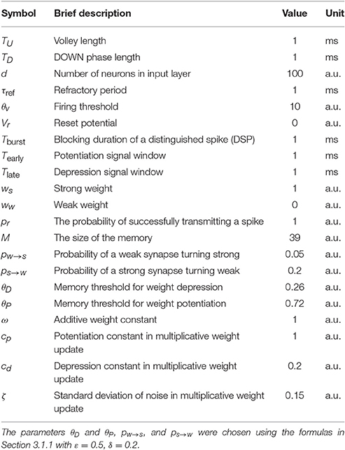
Table 1. Summary of the model parameters and the default values in the model without leak.

TABLE 2

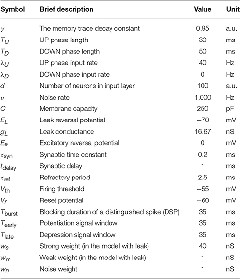
Table 2. Summary of the model parameters and the default values in the model with leak.

TABLE 3

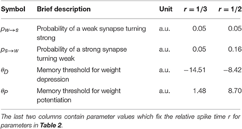
Table 3. Summary of plasticity parameters.

3. Results

3.1. Mathematical Analysis

3.1.1. Mechanism of Normalization

We start our analysis by deriving some formal results in the model without leak. We restrict our analysis to the scenario of a single neuron which receives d excitatory synaptic inputs from presynaptic neurons in a population I, of which d_s are strong. We show that there is an equilibrium input of $d_s^{*}$ strong synapses such that when the total input weight is ≫ $d_s^{*}$, then all synapses have a high chance to decrease their weights. On the other hand, if the total input weight is ≪ $d_s^{*}$, then all synapses are more likely to increase their weights. Thus, the equilibrium $d_s^{*}$ is stable. The analysis also shows an interval around $d_s^{*}$ in which changes of the input weights happen only with very low frequency per volley.

For a single synapse, the total input weight of the postsynaptic neuron determines the expected ratio of potentiation to depression signals. We capture this property by deriving the probability that a synapse receives a potentiation signal instead of a depression signal as a function of the input weight. First, recall that each presynaptic neuron emits exactly one spike per input volley which, in the generic scenario, may be transmitted to the postsynaptic neurons by some probability p_r ≤ 1 (Section 2.1) and, therefore, the postsynaptic neuron spikes at most once per volley. Hence, a potentiation (depression) signal corresponds to a pre/post (post/pre) spike pair within a volley. It should be noted that learning signals are only triggered if both the presynaptic neuron j and the postsynaptic neuron spike and, therefore, one needs to condition on a postsynaptic spike. Furthermore, recall from Equation (3) that the memory of the synapse is the moving average of the number of potentiation signals amongst the last M learning signals. These signals can be viewed as M Bernoulli random variables, where the probability of them being 1 (0) corresponds to the probability of a potentiation (depression) signal. Denote by X the number of strong synapses that transmit a spike in a volley. The postsynaptic neuron spikes if X ≥ θ_v. For a synapse from the j-th input neuron, when d_s out of d synapses are strong, X is binomially distributed such that X ~ Bi(d_s, p_r); accordingly, the probability of the synapse receiving a potentiation signal instead of a depression signal is given by the following expression:

$\mathrm{Pr}[\text{pot}.\text{ signal}]=\{\begin{array}{ll}{p}_{{}_{\text{early}}}^{\prime }(d_s)\equiv \frac{1}{\mathrm{Pr}[X\ge {\theta }_v]}·{\displaystyle \sum _{i={\theta }_v}^{d_s}\frac{{\theta }_v}{i+1}}·\mathrm{Pr}[X=i]\hfill & \text{if }{w}_j(t)=w_w,\hfill \\ p_{\text{early}}(d_s)\equiv \frac{1}{\mathrm{Pr}[X\ge {\theta }_v]}·{\displaystyle \sum _{i={\theta }_v}^{d_s}\frac{{\theta }_v}{i}}·\mathrm{Pr}[X=i]\hfill & \text{if }{w}_j(t)=w_{\text{s}}.\hfill \end{array}(14)$

It thus follows that if the pre- or postsynaptic neuron do not spike in a volley, the memory of the synapse does not change. Hence, the probability of a depression signal is 1−Pr[pot. signal]. The expressions in Equation (14) are shown in Figure 2A for deterministic synapses (p_r = 1, orange) and probabilistic synapses (p_r = 0.5, purple). The small difference between a weak and a strong synapse is caused by the factor $\frac{{\theta }_v}{i}$ for strong synapses and $\frac{{\theta }_v}{i+1}$ for weak ones. For strong synapses this factor corresponds to being amongst the first θ_v input signals out of i strong input signals whereas for weak synapses this factor corresponds to the signal arriving before any of the first θ_v strong input signals where the number of possible places in the order is i + 1.

FIGURE 2

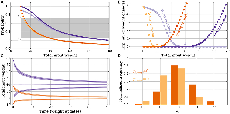
Figure 2. Principles of the intrinsic homeostasis mechanism in the model without leak. Orange curves correspond to a setting with “deterministic” synapses, which reliably transmit spikes, and the purple curves correspond to a setting with “probabilistic” synapses that transmit spikes with probability p_r = 0.5. (A) Probability of a potentiation signal conditioned on the postsynaptic neuron spiking and the synapse being reliable. The gray area corresponds to the value of the memory trace where synapses neither potentiate nor depress. (B) Expected drift toward the stable input weight in each weight update as a function of the total input weight. The arrows correspond to the stable input weights to which the input weight converges in the two settings (the stable state). (C) Convergence to the stable input weight for three different starting conditions in each setting, where one is the stable state. The curves represent the mean over 50 trials and the envelope corresponds to a standard deviation estimate. (D) The total input weight, which is the same as the number of strong synapses d_s, distribution for deterministic synapses after applying 200 weight updates (darker orange) when d_s = 30 before the first weight update. The total input weight distribution is similar to a setting where potentiation is forbidden (p_w→s = 0, lighter orange), which illustrates that the negative feedback does not undershoot the stable state by much. For all panels, M, θ_D and θ_P, p_w→s, and p_s→w are set as in Table 1.

The memory trace m(t) from Equation (3) is an unbiased estimator of Pr[pot. signal] from Equation (14). Furthermore, the probability depends in a monotone fashion on d_s (Figure 2A). This monotone dependence is the principle behind the intrinsic homeostasis effect of the learning rule which allows a synapse to estimate if the total input weight toward the target neuron is too large or too small by just observing and keeping track of recent spike pair orders within a volley. This mechanism results in a stabilizing effect on d_s that we quantify below.

In the model without leak, recall that we apply the weight update rule after every L-th volley. For deterministic synapses, we set L = M. This assumption makes the weight updates independent and, thus, greatly simplifies analysis (see Appendix in Supplementary Material). In the setting with probabilistic synapses, this property holds with high probability by choosing L a bit larger. There, we set $L=\frac{2M}{p_r·Pr\left[X\ge {\theta }_v\right]}$ where, as above, X is the number of synapses that transmit a spike. L depends on d_s for probabilistic synapses because the target neuron cannot be reliably activated if d_s is small.

Denote by Δ_s→w(d_s) (Δ_w→s(d_s)) the number of strong (weak) synapses that turn weak (strong) after applying the weight update rule. Recall that the weights are binary 0 and 1 in the model without leak, so the number of strong synapses is the same as the total input weight. The expected number of weight changes of each type is given by

$𝔼[{\Delta }_{s\to w}(d_s)]=\mathrm{Pr}[Bi(d_s,p_{\text{early}}(d_s))\le {\theta }_{D}M]·d_s·p_{s\to w},(15)$

$\begin{array}{l}𝔼[{\Delta }_{w\to s}(d_s)]=\mathrm{Pr}[Bi(d-d_s,p_{\text{early}}^{\prime }(d_s))\ge {\theta }_{P}M]\\ ·(d-d_s)·p_{w\to s}.& (16)\end{array}$

The expected number of weight changes of each type is shown in Figure 2B for deterministic (orange) and probabilistic synapses (p_r = 0.5, purple). The total input weight change (or “weight drift”) after a learning step is given by

${\Delta }_{w\to s}(d_s)-{\Delta }_{s\to w}(d_s).(17)$

For ε > 0, the expected number of weight changes Δ_w→s(d_s) + Δ_s→w(d_s) for a fixed number of strong input synapses can be bounded by choosing

${\theta }_D=(1-\epsilon )·p_{\text{early}}(d_s)\text{and}{\theta }_P=(1+\epsilon )·p_{\text{early}}^{\prime }(d_s),(18)$

and for some δ > 0 by choosing

$M=\lceil \frac{3\log ({\delta }^{-1})}{{\epsilon }^2{p}_{\text{early}}^{\prime }(d_s)}\rceil .(19)$

A detailed derivation of Equation (19) may be found in the Appendix (Section A2 in Supplementary Material). For this choice of d_s, the expected fraction of synapses that change their weight is less than δ; i.e., 𝔼[Δ_w→s(d_s) + Δ_s→w(d_s)] ≤ δd. It may be noted that this choice of M is independent of the parameters p_s→w and p_w→s. Their roles in the learning rule are simply to reduce the weight drift. Details on how to choose them are given in Section 3.1.2.

In the following, we argue that in the model with leak, the memory trace is a biased estimate of the expected relative spike time r of a DSP within an UP phase. Because of this feature we will refer to the learning rule as the spike latency normalization (SLN) rule. Assume we are in a static setting where the weights are fixed such that the expected relative spike time is r. Let Y_i denote the result of the i-th learning signal: 1 if it was a potentiation signal and 0 otherwise. By ignoring the effect of a specific input neuron on the spike time of the post neuron (which is valid if θ_v is large with respect to w_s) and by assuming that the input neuron spikes only once in the interval [0, T_U] (which is valid if T_U is small compared with 1/λ_U), a synapse expects a potentiation signal with probability r. That is, the variables Y_i can be assumed to be Bernoulli random variables with parameter r. The expected value of the memory trace after ℓ learning signals depends linearly on r and is given by

$\begin{array}{ll}𝔼\left[m\left(t\right)\right]={\displaystyle \sum _{i=0}^{\ell -1}}𝔼\left[{\gamma }^i\left(2Y_i-1\right)\right]={\displaystyle \sum _{i=0}^{\ell -1}}{\gamma }^i\left(2r-1\right){\displaystyle \underset{}{\overset{\ell \to \infty }{\to }}}\frac{2r-1}{1-\gamma }.& (20)\end{array}$

Since the trials are independent, the variance of the distribution can also be easily computed and equals

$\begin{array}{c}\mathrm{\text{Var}}\left[m\left(t\right)\right]={\displaystyle \sum _{i=0}^{\ell -1}}\mathrm{\text{Var}}\left[{\gamma }^i\left(2Y_i-1\right)\right]\\ ={\displaystyle \sum _{i=0}^{\ell -1}}{\gamma }^{2i}4r\left(1-r\right){\displaystyle \underset{}{\overset{\ell \to \infty }{\to }}}\frac{4r\left(1-r\right)}{1-{\gamma }^2}.& (21)\end{array}$

An example of the memory trace distribution is presented in Section 3.2. Furthermore, in Section 3.2.5 we show the expected value of the memory trace 𝔼[m(t)] as a function of d_s for a fixed UP phase length T_U. 𝔼[m(t)] decreases monotonously as a function of d_s. This monotone dependence is the principle behind the intrinsic homeostasis mechanism just as p_early is in the model without leak.

3.1.2. Convergence, Fast Homeostasis, and the Random Spike Order Assumption

In the model without leak, our rule converges to a value $d_s^{*}$ of the total input weight that represents the stable state (or attractor) of the learning process. This state minimizes the expected learning error, which may be quantified by the absolute value of the mean weight drift, that is

$\begin{array}{ll}{d}_s^{*}\equiv {\displaystyle \underset{d_s}{arg min}}𝔼\left[|{\Delta }_{w\to s}\left(d_s\right)-{\Delta }_{s\to w}\left(d_s\right)|\right].& (22)\end{array}$

The stable state is shown with an arrow in Figure 2B. Equations (15) and (16) show that the stable state depends on the parameters θ_P, θ_D, p_s→w, and p_w→s.

In the previous section, M, θ_P, and θ_D were chosen to enforce low expected weight change in some state d_s. We will apply these choices to the steady state $d_s^{*}$. Observe that since 𝔼[Δ_w→s(d_s)] is a decreasing function and 𝔼[Δ_s→w(d_s)] is an increasing function (Figure 2B) we can scale both expectations independently by changing p_w→s and p_s→w, respectively. In this way, $d_s^{*}$ can be adapted.

Starting with $d_s>(1+2\epsilon )d_s^{*}$, it may be shown that (Appendix A3 in Supplementary Material) the expected number of weight updates T applied, until $d_s<(1+2\epsilon )d_s^{*}$ is upper bounded as follows

$𝔼[T]\le \frac{1}{(1-2\epsilon )·p_{s\to w}}·\left(\frac{1}{d_s^{*}}+\log (d_s-(1+2\epsilon )d_s^{*})\right).(23)$

That is, the average number of weight updates is logarithmic in the distance from the target value and inversely proportional to p_s→w, which is the probability of a strong synapse turning weak when m(t) < θ_D. To avoid dangerous oscillations on synaptic weights however, this latter probability should be small so as to prevent the total input weights from dropping to 0. A similar consideration, could also be made for p_w→s insofar as a large value of this probability could result in an overshooting (i.e., strong global potentiation) of synaptic weights, with the important difference however, that, in our formulation, strong potentiation still allows the postsynaptic neuron to fire, whereas strong depression would ultimately result in the shutdown of synaptic inputs. In this catastrophic scenario, the postsynaptic neuron would not be able to fire further, and would become disconnected.

To avoid this possibility and unnecessary weight fluctuations, we present a heuristic criterion to choose p_s→w and p_w→s which allow to upper bound the expected weight change by $\lceil {\epsilon }_1{d}_s^{*}\rceil$ if $ds\in [(1-2{\epsilon }_1)d_s^{*},(1+2{\epsilon }_1)d_s^{*}]$ for some ε₁ > 0. For $d_s=(1+2{\epsilon }_1)d_s^{*}$ the expected number of synapses that depress when a weight update is applied is given by $𝔼[{\Delta }_{s\to w}((1-2{\epsilon }_1)d_s^{*})]$ as in Equation (16). Similarly, the number of synapses that potentiate in when a weight update is applied is given by $𝔼[{\Delta }_{s\to w}((1-2{\epsilon }_1)d_s^{*})]$ as in Equation (15). To prevent undershooting when $d_s>(1+2{\epsilon }_1)d_s^{*}$, it suffices to choose $p_{s\to w}<\frac{c^{\prime }(d_s^{*}-{\theta }_v)}{d}$ for a sufficiently small c′ (e.g., c′ = 2 in this study). The above conditions translate to setting the model parameters such that:

$p_{s\to w}=\min \left(\frac{c^{\prime }(d_s^{*}-{\theta }_v)}{d},\frac{{\epsilon }_1{d}_s^{*}}{𝔼[{\Delta }_{w\to s}((1+2{\epsilon }_1)d_s^{*})]}\right)(24)$

$\begin{array}{ll}{p}_{w\to s}=\frac{{\epsilon }_1{d}_s^{*}}{𝔼\left[{\Delta }_{s\to w}\left(\left(1-2{\epsilon }_1\right)d_s^{*}\right)\right]}.& (25)\end{array}$

Convergence to a stable state where p_s→w and p_w→s are set as in Equations (24) and (25) is shown in Figure 2C, for both deterministic (orange) and probabilistic (purple) synapses in the model without leak. The distribution of the total input weight at equilibrium is shown for the deterministic synapses in Figure 2D, where it is compared with a setting where potentiation is turned off, i.e., where the rule only provides negative feedback. The result in Figure 2D shows that if negative feedback is the only requirement, then it suffices to use the memory trace exclusively for weight depression. If the input to the neuron increases too much, e.g., through some other form of short-term Hebbian learning, then the negative feedback provided by the memory mechanism of the strong synapses can quickly reduce the input weight back to a stable state without undershooting it. In both settings described above, the initial total input weight was d_s = 30 and the distribution in the figures is shown after 200 weight updates have been applied.

Figure 3A shows how the stable state $d_s^{*}$ is affected by probabilistic synapses. In particular, in this case $d_s^{*}$ increases by a factor of $p_r^{-1}$ if other parameters remain fixed. The intuition behind this relation comes from two observations. First, for that state, the expected total input weight is the stable state for deterministic synapses. Second, if the number of strong synapses d_s is large enough, then the total input X = Bi(d_s, p_r) is concentrated around its mean μ_X = d_sp_r with standard deviation ${\sigma }_X=\sqrt{d_s{p}_r(1-p_r)}$. Asymptotically for growing θ_v, d_s, and d, the main contribution in the sum in Equation (14) comes from terms close to the mean of the form

$\begin{array}{l}\frac{{\theta }_v}{{\mu }_X\pm \Theta \left({\sigma }_X\right)}=\frac{{\theta }_v}{{\mu }_X\left(1\pm \Theta \left({\sigma }_X^{-1}\right)\right)}=\left(1\mp \Theta \left({\sigma }_X^{-1}\right)\right)·\frac{{\theta }_v}{{\mu }_X}\\ =\left(1\mp \Theta \left({d_s}^{-1/2}\right)\right)·\frac{{\theta }_v}{d_s{p}_r}.& (26)\end{array}$

FIGURE 3

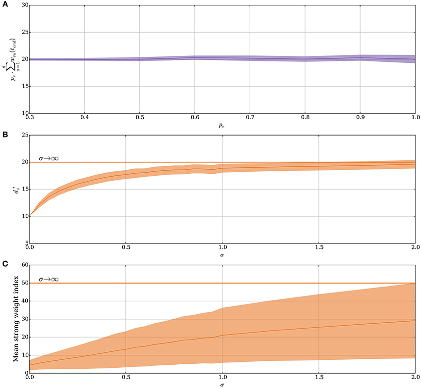
Figure 3. Noisy input and the random order assumption in the model without leak (Section 3.1.2). (A) The stable state $d_s^{*}$ scales by 1/p_r for probabilistic synapses. The initial value of d_s is set to 20/p_r for each p_r and the plot shows the mean value of d_s · p_r after 50 weight updates over 100 trials. (B–C) From a fixed order to a random order. Spike order distributions that are not uniform are considered in these panels. The parameter σ brings them from a fixed order (σ = 0) to a uniform order (σ → ∞). (details are explained in Section 3.1.2). Initially, each synapse is strong independently, with probability 4θ_v/d. (B) Small variability brings the stable state $d_s^{*}$ close to same state as when the spike order is uniform. (C) The plasticity mechanism prefers early neurons when σ is small. This is reflected by the mean index of the strong synapses, which are indexed from 1 to d in ascending order of expected spike time. However, as σ increases, the early neurons become less distinguishable from later neurons. In (B,C) each data point is the mean of 250 trials, where for each trial 250 weight updates are simulated. For all panels, the plasticity parameters are chosen as in Table 1 and the envelopes represent standard deviation estimates.

In Equation (26) above, the notation f = Θ(g) means that f is bounded by g both above and below asymptotically.

Our hitherto analysis has considered the input order to be uniformly distributed (i.e., “random order” assumption), yet one may also ask how the SLN rule performs if this assumption is relaxed. Indeed, spikes are known to have a precise repeating temporal structure in some cortical areas related to sensory processing (Bair and Koch, 1996; Heil, 1997; Fellous et al., 2004) and standard STDP is known to tune to the first spike for such repeating spike patterns (Guyonneau et al., 2005). To model the transition from an orderly spike distribution to a uniform one the expected relative spike time of every input neuron in a volley is fixed but the deviation of the spike time is varied. Formally, for the i-th neuron a normal random variable $Z_i~{N}(i/d,{\sigma }_Z)$ is sampled. These variables impose an order on the input spikes within a volley in a natural way. For the resulting order, the input neurons spike in an equi-spaced manner. This approach is valid since we ignore membrane leakage and, therefore, the spike order is the only temporal structure that has any influence on the distribution of potentiation and depression signals. For σ_Z = 0, the ordering is fixed as 1, 2, …, d and for a growing σ_Z, the ordering approaches a uniform distribution. Figure 3B shows how this choice of input spike distribution affects the stable state $d_s^{*}$. Not surprisingly, if the order is fixed (σ_Z = 0), then only the first θ_v synapses get strengthened as was the case in Guyonneau et al. (2005) where classic STDP by a repeating spike pattern turned the neuron into a detector for the start of the pattern. However, already a small value of σ_Z quickly shifts the stable state toward the same one as for a random input order. For σ_Z = 2.0 the first 20 input neurons are close to a random permutation since the probability of the 20th neuron being earlier than the first neuron is approximately 0.47. Figure 3C shows the mean index of strong synapses. Even though the stable state remains close to the same for small values of σ_Z, the early synapses are the ones that are preferably strengthened in agreement with Guyonneau et al. (2005). For other choices of spike order distributions, the negative feedback of the intrinsic homeostasis mechanism still applies (Appendix A4 in Supplementary Material).

3.2. Numerical Simulations

3.2.1. Stability in the Model with Leak

As in the model without leak, the number of weight changes in the model with leak is mainly determined by two factors: (i) the number of synapses whose memory trace lies outside the target interval [θ_D, θ_P] and (ii) the weight update parameters p_s→w and p_w→s. How the width of the interval [θ_D, θ_P] affects plasticity is shown in Figures 4A–C, whereas an example of how p_s→w and p_w→s can affect plasticity is shown in Figure 4D. The width of the target interval [θ_D, θ_P] determines how many synapses can change their weight in the stable state. Such intervals are laid over the memory trace distribution in Figure 4A, which was sampled by fixing d_s = 20. The tails of the distribution outside the interval correspond to the synapses that can change their weight. Since these tails fall off exponentially if the learning signals are independent Bernoulli trials, the fraction of synapses that can update their weights in the stable state can be made arbitrarily small by choosing a large interval. It may be noted that the parameter γ also needs to be chosen sufficiently close to 1, which corresponds to choosing M larger in the model without leak. Therefore, one can choose parameters such that a region around the stable state induces almost no weight changes, thus avoiding unnecessary fluctuations of total input weight. However, choosing a large interval also leads to diminished plasticity in regions further away from the stable state (Figure 4B). This suggests that a trade-off exists between synaptic weight plasticity and the time to reach close to the stable state.

FIGURE 4

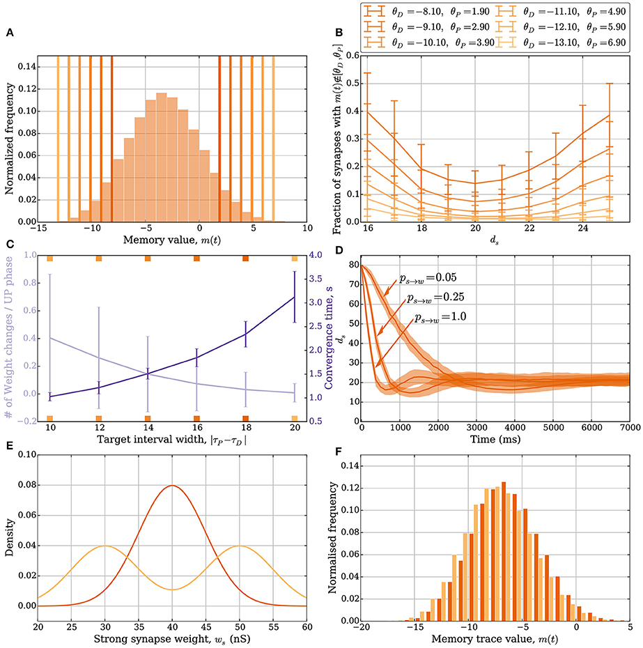
Figure 4. Plasticity vs. stability in the model with leak (Section 3.2.1). (A) Distribution of the memory trace in a static setting, with p_s→w = p_w→s = 0 and d_s = 20 strong input synapses. The colored vertical bars represent the target interval [θ_D, θ_P] used in (B,C). (B) The mean fraction of synapses whose memory trace lies outside the interval [θ_D, θ_P] in a static setting. (C) The trade-off between the number of weight changes in the stable state and convergence time to the stable state. The light purple curve shows the mean number of weight changes per UP phase over all input synapses. The dark purple curve shows the mean time for the weights to converge from d_s = 80 to d_s = 25. The ticks on the x-axis are colored and correspond to the thresholds in (A) and curves in (B). In this setup, the number of strong synapses in the stable state is d_s = 20. This is achieved by choosing p_s→w and p_w→s such that they satisfy the equation d_sp_s→w = (d − d_s)p_w→s; i.e., p_w→s = 0.0625 and p_s→w = 0.25. The error bars represent standard deviation estimates. (D) Comparison of the effect p_s→w and p_w→s have on convergence. In this figure, θ_D = −5.1 and θ_P = −1.1, and three different values of p_w→s (0.05, 0.25, and 1.0) are compared (the corresponding p_s→w values are 0.01, 0.06, and 0.25). If too many synapses change their weight simultaneously because of a small target interval and large weight change probabilities, then the weights can overshoot the stable state and oscillate around it. (E,F) Stability for different weight distributions. (E) Density function for two different weight distributions of the strong synapses. The dark orange is the density function of ${N}(40,5)$, and the light orange is the density function for the random experiment, where we either draw the weight from the distribution ${N}(35,5)$ or ${N}(45,5)$ based on a fair coin toss. (F) The corresponding memory trace distribution for each weight distribution when d_s = 24 in a static setting with p_s→w = p_w→s = 0. By choosing θ_D = −16 and θ_P = 5, the weight remains unchanged for both weight distributions over a period of 50 s and oscillating input (data not shown). In (A) the distribution is obtained by sampling memory traces of all d synapses after a simulation of 500 UP phases in 250 trials. In (B) each data point is the mean of 100 trials. In (C) each curve is the average over 40 trials. In (D) each curve is the average over 200 trials with a data point every 125 ms. For all panels, error bars and envelopes represent standard deviation estimates. In (F) the distribution is sampled from 100 synapses over 200 trials of a 50 second simulation.

Figure 4C shows such trade-off where the orange curve represents the expected number of weight updates per UP phase when d_s = 20 (over all synapses) whereas the purple curve shows the mean time to remain with 25 strong synapses starting from 80. For Figures 4A–C, the parameters p_s→w and p_w→s were set to 0.25. In combination with a small target interval, a bad choice of p_s→w and p_w→s can lead to plasticity over- or undershooting as in the model without leak (see Section 3.1.2). Undershooting the input weight in the stable state is a concern if it results in the weights being too small to activate the target neuron. Overshooting is less of a concern for activation, but it is wasteful since fewer weight updates can be used to reach the stable state. An example of undershooting is shown in Figure 4D, where θ_P = −1.1 and θ_D = −5.1. Over- and undershooting happen in this setting because the memory trace depends on learning signals from the past that are irrelevant when the weights are close to converging. To handle this effect, weight updates can be limited by choosing p_s→w and p_w→s small enough. Furthermore, since input neurons in the model with leak do not always spike in an UP phase only a fraction of the input synapses update their memory trace and trigger the weight update rule. This results in a natural tie-breaking mechanism that prevents all synapses from updating their weights simultaneously.

The SLN rule achieves normalization quickly. Though speed is a desirable property (see the work of Zenke et al., 2013 for a discussion on the necessity of a fast-homeostatic mechanism), it is also important to be energy efficient; that is, the total number of synaptic weight changes should be small. Different synaptic weight distributions can result in the same value of expected relative postsynaptic spike time. A feature of stability in the SLN rule is that this does not result in further weight changes. We highlight these features in Figures 4E,F. Figure 4E shows two different synaptic weight distributions for the strong weight synapses. One is normally distributed with mean 40 nS and standard deviation 5 nS (dark orange). The other is obtained by sampling from a normal distribution as well, with the same standard deviation, by first flipping a fair coin to decide if the mean should be 35 or 45 nS (light orange). The resulting distribution of the memory trace is shown in Figure 4F when p_s→w = p_w→s = 0 and d_s = 24. By setting θ_D = −16 and θ_P = 5, the synaptic weights remain unchanged over 1 min of input activity (data not shown). That is, both weight distributions are stable.

3.2.2. Short vs. Long UP Phases

For short UP phases the SLN rule normalizes the expected relative spike time r of the postsynaptic neuron within an UP phase whereas for long UP phases the rule normalizes the absolute expected latency of the postsynaptic neuron, which is equivalent to normalizing the total input weight in this setting. Figures 5A,B demonstrate how the number of strong input synapses d_s and the relative spike time r change when varying the length of the UP phase if we start with d_s = 25 and run the process until the weights converge. We use a log-scale for the x-axis to show data for very long UP phases. Figure 5A shows that for long UP phases the input weight is normalized whereas Figure 5B shows that for short UP phases the relative spike time is normalized. We show UP phases of length 20.0, 25.0, 30.0, 35.0, 40.0, 45.0, 50.0, 60.0, 80.0, 100.0, 500.0, and 1000.0 ms. The length of the down phase is set to 1000.0 ms and we set T_burst = 1000.0 such that there can be only one DSP per UP phase. We use the plasticity parameters in Table 3 for r = 1/3 (dark purple) and r = 1/2 (dark orange) where the lighter colored curves correspond to a setting with p_w→s = 0.0 as in Section 3.1.2. The schematic in Figure 5C explains the reason for this difference. The figure shows two different rate functions with short (30 ms) and long (500 ms) UP phases. Postsynaptic spikes are drawn on top of the rate function for reference where darker spikes represent DSPs. The windows for potentiation and depression signals are drawn in black over the DSPs. For short UP phases the windows for potentiation and depression signals cover the whole UP phase. In this setting, the fraction of potentiation signals represents the relative spike time within an UP phase. In contrast, for long UP phases, the window of depression lies completely within the UP phase. To compensate for more depression signals the input weight needs to decrease such that the ratio of potentiation to depression signals is within the target regime. Figure 5D shows the weight over time for short UP phases of 30 ms with d_s = 17 at t = 0 (left panel) and long UP phases of 0.5 s with d_s = 27 at t = 0 (right panel). In both panels the DOWN phases are of length 1 s. We use the plasticity parameters for r = 1/3 in Table 3 which corresponds to the dark purple curve in panels A-B. Each timescale captures 400 UP phases and we show 20 example runs with one highlighted in orange for clarity.

FIGURE 5

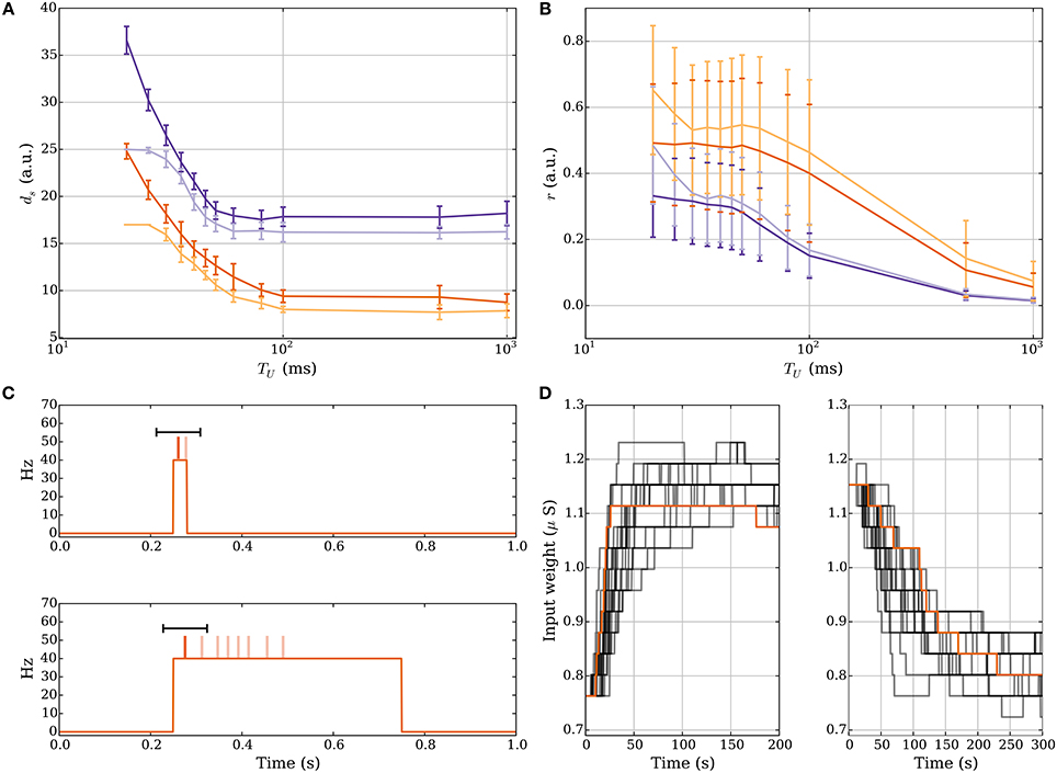
Figure 5. Comparison of short and long UP phases. (A,B) Dependence of number of strong input synapses d_s and relative spike time on the lengths of UP phases. We set T_D = 1000.0 ms and we set T_burst = 1000.0 such that there can be only one DSP per UP phase. (A) shows that for long UP phases the mechanism normalizes d_s. (B) shows that for short UP phases the mechanism normalizes the relative spike time r within an UP phase. (C) Depression is stronger for sufficiently long UP phases. For two different rate functions the postsynaptic spikes are drawn on top of an UP phase where darker spikes represent DSPs. The black bar represents the learning windows. The time window of the depression signal is completely within the UP phase if the UP phase is long. This increases the expected number of depression signals. To compensate, the input weight needs to decrease in order to correct the ratio of potentiation to depression signals. (D) Weight change for short UP phases of 30 ms with d_s = 17 at t = 0 (left panel) and long UP phases of 0.5 s with d_s = 27 at t = 0 (right panel). We show 20 example runs with one highlighted in orange for clarity.

For long UP phases we chose T_burst sufficiently large to permit only one DSP per UP phase. However, for short DOWN phases this leads to a DSP blocking first spikes of subsequent UP phases becoming DSPs. As an alternative, one can assume that a DSP is only triggered if the membrane potential was recently in a low state of activity and a DSP blocks further DSPs until a low activity state is reached again. One can further assume that spike pairs are only considered to trigger learning signals if the subthreshold activity remains above some threshold between both spikes. This voltage based approach fixes the issue above with short DOWN phases and it implies that for constant or high rate input (as we study in Section 3.2.6), where the subthreshold potentiation remains large, neither the memory nor, hence, the synaptic weight, would change.

3.2.3. Heterogeneous/Multimodal Weights

The SLN rule also works for heterogeneous and multimodal synapses although the exposition so far was restricted to binary synapses. This more general scenario is discussed in the model without leak of mere SIF neurons, with results from simulations presented in Figure 6.

FIGURE 6

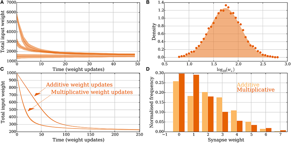
Figure 6. Heterogeneous and multimodal weights in the model without leak (Section 3.2.3). (A,B) Heterogeneous weights. (A) Input convergence with the spike threshold θ_v adapted to the synaptic weights. (B) Comparison between the distribution of strong synaptic weights (lognormal distribution, shaded) and the strong weights after convergence (dots). (C,D) Multimodal synapses. Two different weight update rules are presented: one additive and one multiplicative (see Section 2.5 for details). (C) Convergence for the two different setups where all the synapses start with weight 10 and θ_v is set to 100. (D) The input weight distributions are compared for the multimodal weight update rules in (C) after 250 extra weight updates. The additive weight update rule produces a bimodal weight distribution whereas the multiplicative one produces a unimodal distribution. None of the update rules imposes a hard upper bound on the weights and all resulting weights are less than 10, which was the starting weight of the synapses. For all panels, the parameters were chosen as in Table 1 unless otherwise specified. In (A,C) each curve is the mean of 30 and, respectively, 100 trials; the envelopes represent a standard deviation estimate. In (B) the distribution is obtained from 5.000 trials, where in each one 50 weight updates were simulated.

In the setting with heterogeneous weights w_w = 0 for all synapses, whereas w_s is drawn independently for each synapse from a distribution as in Barbour et al. (2007). The distribution is the one reported in Loewenstein et al. (2011), where $w_s=e^{{N}(\mu ,\sigma )}$ with μ = 1.74 and σ² = 0.1002. The mean of the distribution is 10^μ+σ2/2 ≈ 5.726. To compare this with the binary weight setting where θ_v = 10, the threshold is set to ${\theta }_v=10·e^{\mu +{\sigma }^2/2}$. Convergence to a stable state is shown in Figure 6A. Initially 20, 40, or 80 synapses are strong. After convergence, the weight distribution of synapses selected to be strong is compared with the lognormal distribution from above (Figure 6B). The empirical distribution is composed of 5.000 trials and the neuron and synapse parameters (except θ_v and the weight) are in Table 1.

Figures 6C,D compare convergence and weight distribution for the two different setups from Section 2.5. The plasticity parameters are the same as in Figure 2. The additive weight update rule is slower to converge since the weight updates are smaller for large input weights compared with the multiplicative rule. Figure 6D shows that in this specific setting, the synaptic weights do not need to be explicitly upper bounded. This holds because the input arrives in a random order and the causative effect of a single synapse is small. Figure 6D also shows that the additive (multiplicative) weight update rule converges to a bimodal (unimodal) distribution. Both uni- and bimodal distributions have been observed for earlier plasticity rules, whereas bimodal distributions are considered a sign of competition since some synapses being strong force others to be weak.

3.2.4. Robustness of Convergence

We show that the stability of the rule does not depend on the exact input parameters and that perturbations do not qualitatively affect it. Figure 7 illustrates this robustness in the model with leak. The different panels show two different plasticity parameter settings that correspond to r = 1/3 (purple) and r = 1/2 (orange) in Table 3. In Figures 7A–C, the lengths of UP and DOWN phases (T_U and T_D), and the number of inputs d are varied. The process is first simulated for 200 UP phases starting with d_s = 25 such that the input weight reaches the stable state. The data in the figures is based on UP phases 201–400 in 40 trials. Figure 7A shows that the SLN rule fixes the relative spike time r of the postsynaptic neuron. The stable value of r mildly depends on T_U, which arises from the choice of synaptic delay t_delay = 1 ms. To explain this, denote by t₁ the spike time of the pre spike which triggers the postsynaptic spike at time t₂. Any presynaptic neuron that spikes in the interval (t₁, t₂) receives a potentiation signal, which leads to a mild bias toward potentiation that is stronger for short UP phases. The variable r determines the number of spikes per UP phase (Figure 7B) since the number of spikes is inversely proportional to r. The number of spikes per UP phase has a mild dependence on T_U since the refractory period has a stronger effect for short UP phases and the reset potential makes repeated spikes easier. Figure 7C shows that the intrinsic homeostasis mechanism does not fix the rate of the output neuron since it is determined by T_U and T_D.

FIGURE 7

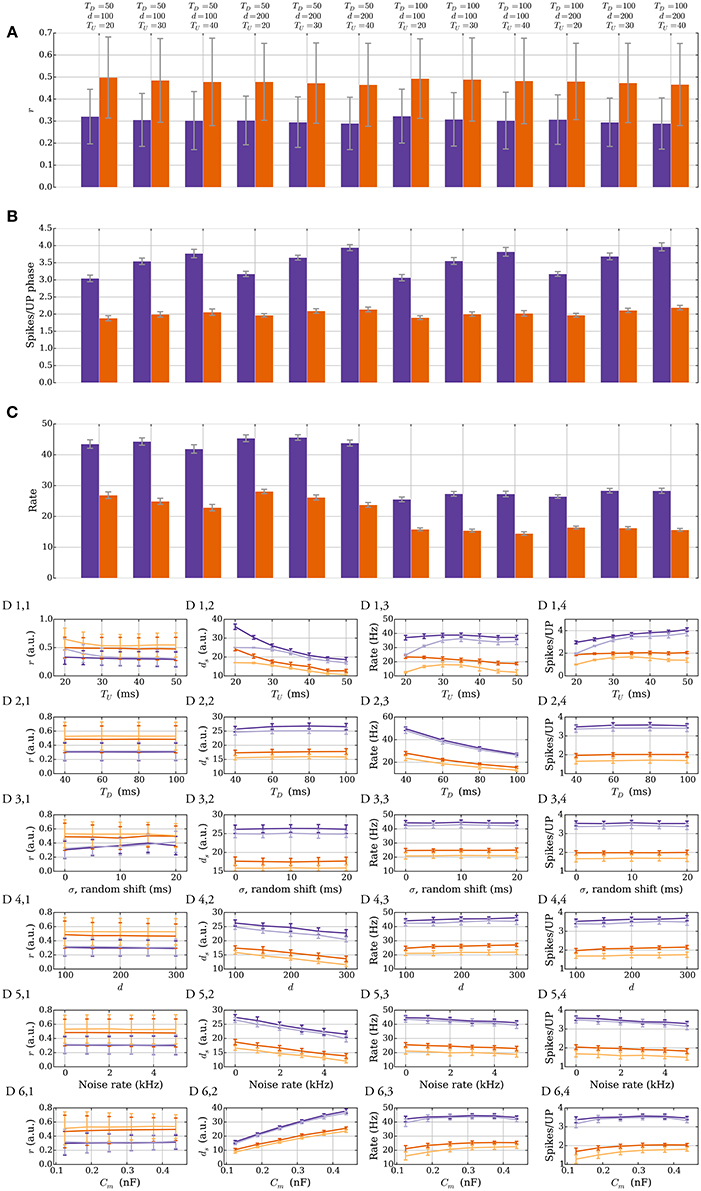
Figure 7. Robustness against varying input parameters in the model with leak (Section 3.2.4). (A–C) Results for two different sets of plasticity parameters corresponding to r = 1/3 (purple) and r = 1/2 (orange) in Table 3 are shown. Three parameters of the input are varied: the length of an UP phase T_U; the number of input neurons d; and the length of a DOWN phase T_D. (A) r, the expected time of the first postsynaptic spike within an UP phase scaled by the UP phase length. The plasticity parameters fix r; thus, varying the input parameters has a negligible effect on it. (B) Variations in the number of spikes per UP phase. The number of spikes per UP phase depends on r, but it also has a mild dependence on the refractory period and the reset potential, which explains the variations seen when varying T_U. (C) Output rate variations. The rule does not fix the output rate of a neuron: the rate depends mainly on T_U and T_D. (D) Single parameter variations. Variations for six different parameters are shown. The darker colored curves correspond to the same plasticity parameters as in the top three panels, and the lighter colored curves correspond to a setup with no positive feedback (p_w→s = 0). The first row is for T_U, the second is for T_D, the third is for random phase shifts of the input neurons, the fourth is for d, the fifth is for the noise rate ν, and the sixth is for the membrane capacitance (for details see Section 3.2.4). The orange curves start with d_s = 17 and the purple curves start with d_s = 25. Each data point in (A–C) is the mean of 40 trials and in (D) the mean of 10 trials. The error bars represent standard deviation estimates. For each trial, the process was simulated for 200 UP phases to reach the stable state and then the data points were collected over a continued simulation of 200 UP phases (r, rate, spikes per UP phase), or at the end (d_s).

Figure 7D shows the effects of single parameter variations. The darker colored curves correspond to the same plasticity parameters as in Figures 7A–C and the lighter colored curves correspond to a setting without positive feedback, i.e., when p_w→s = 0 (see Section 3.1.2 for a similar setting in the model without leak). Observe that most single parameter variations in this setting do not cause large plasticity undershooting. The main effects caused by T_U and T_D are covered above so we do not cover the first two rows here (the lower order effects of T_U on r are covered in the next paragraph). The third row corresponds to varying the phase shift of the inputs randomly (see Section 2.2). For that setting we replace T_U by T_U + σ in the definition of r. We see r increase due to a reduced input weight like we observed for more orderly input distributions in the model without leak (see Section 3.1.2). Rows four and five correspond to the number of input neurons and noise rate, respectively. Variations on both of these parameters have similar effects, as increasing these parameters helps activate the target neuron. Consequently, d_s must decrease to compensate (D 4,2 and D 5,2). The last row corresponds to varying the membrane capacitance C_m. Increasing the capacitance decreases the leak conductance, but it also reduces the excitatory synaptic conductance, which makes it harder to activate the neuron. Despite large variations, r remains fixed.

To conclude this section, let us consider the lower order effects from T_U, d, and noise strength on r. For simplicity assume that θ_P and θ_D are chosen such that a δ fraction of the strong (weak) synapses satisfies m(t) ∉ [θ_D, θ_P] in the stable state. For the corresponding input weight $d_s^{*}$, the parameters p_s→w and p_w→s satisfy

$\begin{array}{rc}\left(d-d_s^{*}\right)·\delta ·p_{w\to s}=d_s^{*}·\delta ·p_{s\to w}.& (27)\end{array}$

However, if we increase T_U, the noise, or d, then $d_s^{*}$ will change to compensate such increase. If $d_s^{*}$ needs to decrease by x to obtain the correct value of r, then the left-hand side in Equation (27) increases by xδp_w→s whereas the right-hand side decreases by xδp_s→w. Therefore, the number of strong synapses will not converge to exactly $d_s^{*}$ − x. However, if the interval [θ_D, θ_P] is large enough such that δ is small, then this effect is reduced.

3.2.5. All-to-All vs. Distinguished Spikes

The principle of sampling the expected spike time of the postsynaptic neuron in an UP phase also applies if the synapse considers all pre/post and post/pre spike pairs within an UP phase to constitute potentiation and depression signals. In this section, we show the advantage of using a single DSP: it improves the signal-to-noise ratio. Furthermore, later postsynaptic spikes in an UP phase have more preceding presynaptic spikes in the UP phase and, thus, carry a weaker signal. Figure 8A compares the memory value for these two rules in a static setting where synapses have fixed weights. The figure shows the advantage of DSPs. They reduce the variance of the memory trace and increase its range, which makes the two different values of d_s more distinguishable. It may be noted that both versions of the rule perform similarly for small values of d_s because then only one postsynaptic spike is expected (i.e., both act as with DSPs). However, as d_s grows, and the postsynaptic rate increases the memory traces for the two rules start to differ. The difference arises from the fact that if the postsynaptic neuron spikes for example five times, then the update to the memory trace for DSPs is only −1 or 1 (for a single presynaptic spike), whereas it can range from −5 to 5 in the all-to-all setting. Furthermore, depression signals are more common in the DSP setting for large d_s, whereas potentiation dominates in the all-to-all setting. This effect comes from the spike time distribution of the postsynaptic neuron within an UP phase.

FIGURE 8

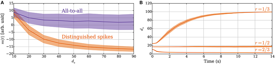
Figure 8. (A) Advantage of DSPs (Section 3.2.5). With DSPs in the model with leak, the variance of the memory trace is considerably smaller than for an all-to-all rule. The curves show the mean memory trace value when varying the number of strong inputs d_s in a static setting with p_s→w = p_w→s = 0. The orange curve corresponds to the SLN rule. The purple curve corresponds to a rule where all pre–post and post–pre spike pairs within an UP phase trigger learning signals. (B) Constant rate input at 40 Hz in the model with leak (Section 3.2.6). The two different sets of plasticity parameters from Table 3 are compared. For each setting, the number of strong synapses d_s is initially set in the stable state for the oscillating input. For the r = 1/3 parameters, all the synapses increase their weights since the synapses receive potentiation signals half of the time instead of one-third of the time, which they expect. For the r = 1/2 parameters, there is no such disagreement and for the r = 2/3 parameters it is the opposite and the input weight decreases to a point where activation becomes unreliable. In (A) the mean is taken after a 50-s-simulation over 10 trials, where in each trial samples are taken from all 100 synapses. In (B) the curves show means of 50 trials. In both panels the envelopes represent standard deviation estimates.

3.2.6. Fixed Rate Input

So far we assumed that the input signal oscillates between high and low states of activity. One may also ask, however, what happens if the input rate is constant, which is a common assumption in modeling studies (Burkitt, 2006a). In this regard, the behavior of the SLN rule is determined by the ratio of potentiation and depression signals as before. However, for constant input rate the rule does not have a frame of reference to measure the input strength anymore. The ratio of potentiation and depression signals is, therefore, determined by the parameters T_early and T_late. If we choose the parameters θ_P, θ_D such that the memory trace lies entirely within the interval [θ_D, θ_P] for constant input rate, then the weights do not change. However, if a larger fraction of the memory trace distribution lies below θ_D than above θ_P, then the total input weight decreases up to a point where activation of the neuron becomes unreliable. For the opposite case, all the synapses get strengthened, which is not desirable. Figure 8B illustrates this by showing how the system responds to constant input for three different sets of plasticity parameters. For parameters that result in r > 1/2, the weights decrease to a point where the target neuron shows almost no reaction to the input. Indeed, this seems a reasonable response as such an input does not carry any information. On the other hand, for parameters that result in r < 1/2 the weights and the firing rate of the target neuron grow to the maximum value, which is undesirable if the activity of the neuron should be limited. These observations indicate that the parameters should fix r to be at most 1/2, which corresponds to several spikes of a neuron in an UP phase (≈ 1/r) and is in good agreement with experimental findings (Connors and Gutnick, 1990). Furthermore, the synapses should not expect disproportionally more potentiation signals than depression signals.

4. Discussion

There are two forms of homeostasis prominently discussed in the literature. First, there is the concept of normalization (or scaling) of total input weights with respect to a target total weight (Von der Malsburg, 1973). Second is the concept of rate normalization, where rate of the postsynaptic neuron should stay within a target regime. The latter option is regarded to be more plausible than the former, insofar as it can be implemented locally at the level of a single synapse so that the computation is restricted to the sole information available at that synapse. In contrast, the first option requires computation of the total input weight which was not considered a synapse specific computation but rather a neuron specific computation (Zenke et al., 2013). In this paper, we introduce a third option: a fast-acting local homeostasis mechanism that normalizes the expected spike time of a neuron in an UP phase of an oscillatory input rate function. Two independent studies have identified the order of the time scale for fast homeostasis to be seconds (El Boustani et al., 2012; Zenke et al., 2013), which is well within the parameter regimes of the SLN rule presented in this paper (for a recent review see Zenke and Gerstner, 2017). Furthermore, normalization is applied on a fast time scale in most, if not all, computational studies (Chistiakova et al., 2015). The fact that the SLN rule is Hebbian challenges the belief that regulation of neuronal excitability is difficult if synapses are modified independently by such rules (Abbott and Nelson, 2000). Furthermore, for long UP phases the rule results in input weight normalization which challenges the belief that estimating the input weight cannot be done through local synaptic computation. Moreover, the rule is energy-efficient in the sense that the synaptic weights do not change in the stable state for parameters favoring stability. In particular, if the postsynaptic neuron is spiking with the correct expected relative spike time, then the homeostasis mechanism does not intervene. Hence, the weights do not converge to a unique distribution.

4.1. Related Literature

4.1.1. Related Metaplasticity Rules

The SLN rule bears some resemblance to the metaplasticity rule proposed by Brader et al. (2007). Common to both rules is a synapse specific memory trace represented by a real value which is updated for certain spike events. Other metaplasticity rules depend on discrete states within the synapses such as the synaptic integration rule by Elliott and Lagogiannis (2012) which can be considered a multimodal version of the cascade rule by Fusi et al. (2005). However, these metaplasticity rules have not been studied in the context of SLN for UP/DOWN state input activity where, in particular, the fast and robust weight convergence for such activity has not been demonstrated before.

4.1.2. Volley-Like and Repeating Input Patterns

The effect of standard STDP on spike timing was studied and analyzed in detail in the context of volley-like input spike distributions in Gerstner and Kistler (2002, Chapter 12.2). Furthermore, if the relative effect of potentiation is reduced then STDP leads to convergence of the input weights to a stable distribution for random input activity (Van Rossum et al., 2000). For both these cases, the synaptic weights perform random walks in the stable setting whereas the SLN rule provides a stronger stability guarantee since it implicitly fixes the weights at equilibrium and the weight distribution at convergence is not unique. Hence, the SLN rule is economical in the sense that synaptic weights are only changed when it is necessary which is in agreement with other studies since not all spike pairs necessarily lead to a weight change (Yger and Gilson, 2015).

Other theoretical studies have considered repeating spike inputs as the ones presented in Section 3.1.2. Guyonneau et al. (2005) studied standard STDP for repeated stimulation of a neuron with the exact same spike pattern. Through such repeated exposure the postsynaptic neuron becomes a coincidence detector for the given pattern. Further studies showed that this feature is robust to noise (Masquelier et al., 2008, 2009).

4.1.3. Other Activity Dependent Homeostasis Mechanisms

Perhaps the most prominent example of homeostasis in plasticity models is the BCM rule (Bienenstock et al., 1982). The weight update in the BCM rule normalizes postsynaptic rate by using a threshold which varies slowly with the postsynaptic rate. Nearest-neighbor STDP has been shown to perform a simplified version of this operation, i.e., without the sliding threshold, when pre- and postsynaptic activity is weakly correlated (Izhikevich and Desai, 2003).

Other studies have focused more directly on preventing single weights from being driven to extreme values. Gütig et al. (2003) presented a plasticity model where the plasticity rule is weight dependent and, therefore, leads to an implicit upper bound on synaptic weights through a mixture of additive and multiplicative weight changes. Babadi and Abbott (2010) had an even more implicit approach by shifting the effective STDP temporal window by roughly 2 ms such that pre/post pairs that are close in time lead to depression instead of potentiation. This effect works against synapses with a large causative spiking effect. It may be noted that the same principle can also be applied for the SLN rule.

Another variable which could be controlled through homeostasis is the type of activity in a neural network. In this regard, STDP is known to sustain a stable background state in balanced networks (Kempter et al., 1999, 2001; Song et al., 2000; Van Rossum et al., 2000; Rubin et al., 2001) and to regulate activity (Kempter et al., 1999, 2001; Song and Abbott, 2001; Pfister et al., 2006; Watt and Desai, 2010) but these models have been criticized for parameter fine-tuning (for a review see Chistiakova et al., 2015). Theoretical investigations showed that fast detection of postsynaptic rate changes can solve the problem (Zenke et al., 2013; Yger and Gilson, 2015) but these studies do not consider the scenario of UP and DOWN phases.

It is plausible that homeostatic plasticity is controlled by more than a single mechanism (Tononi et al., 1999; Watt and Desai, 2010) as many alternatives, like we discussed, which have a homeostatic effect on various parameters of neurons or network activity have been proposed (Bienenstock et al., 1982; Rabinowitch and Segev, 2006; Vogels et al., 2011; Remme and Wadman, 2012). It is known that homeostatic plasticity is affected by a complex web of signaling processes many of which are likely undiscovered (Pozo and Goda, 2010) and which might even be shared between, or belong to, different homeostasis mechanisms. As an example, weight normalization is considered biologically plausible because a neuron might have finite resources dedicated to maintaining its synapses, but there is a lack of experimental evidence to support this.

4.2. Biophysical Bases for Memory Traces

For the SLN rule, we require the synapses to hold a trace of learning signals from the past. Some previous learning models depend on a synapse-specific memory trace that represents global information shared by all or many input synapses of a neuron (Brader et al., 2007; Urbanczik and Senn, 2009; Brea et al., 2013, 2016; Urbanczik and Senn, 2014). Several hypotheses propose that some form of memory can reside in a synapse. Min and Nevian (2012) suggest that astrocytes could act as a memory buffer to store previous coincident spike events. Astrocytes could further provide the signal that determines if a synapse should increase or decrease its weight (De Pittà et al., 2016; De Pittà and Brunel, 2016). Another candidate that has been proposed to represent a long-lasting memory trace of past synaptic activity is calcium/calmodulin-dependent protein kinase II (CaMKII) (Hell, 2014). This protein kinase can assume two stable states depending on whether it is phosphorylated (active) or not (auto-inhibited). Earlier results have shown that LTP induction induces a persistent translocation of CaMKII to synaptic spines, causing it to be considered as a form of a long-term memory trace (Otmakhov et al., 2004). Other more short-lived memory traces have also been proposed such as transient neurotransmitter concentrations, like dopamine, which can extend the window of potentiation in STDP and is supported by experimental evidence (Zhang et al., 2009), and the local membrane potential at a synapse (Urbanczik and Senn, 2014).

4.3. Rhythmic Input

The intrinsic homeostasis effect of the SLN rule is designed for input activity that switches between high and low states. Oscillations of activity are ubiquitous in the brain (Reyes, 2003; Buzsáki and Draguhn, 2004), but their exact functional role is still not fully understood. The most prominent hypothesis of the functional role of oscillations in brain activity is the “communication-through-coherence” hypothesis, see the reviews in Fell and Axmacher (2011) and Thut et al. (2012). This hypothesis posits that neural populations communicate through phase-locked oscillations. If the subthreshold potentials of the two populations are phase locked, then the source population can activate the target if it is in an UP state when the signal arrives, which is considered to lead to long-term potentiation. Correspondingly, if the target population is in a DOWN state, then the activation becomes harder and is believed to lead to long-term depression. Recent evidence indicates that retrieval of information in the hippocampus is discretized with respect to slow-wave gamma oscillations and sharp-wave ripple events, which are recognized as the most synchronous patterns in the brain (Pfeiffer and Foster, 2015). However, synchronous and rhythmic activity is also observed during sleep and then the duration of UP and DOWN phases is typically in the order of seconds (Steriade et al., 2001; Jercog et al., 2016). Even though these observations were first made some decades ago (Steriade et al., 1993a,b,c) the functional role of UP and DOWN phases is still not apparent (Vyazovskiy and Faraguna, 2014).

4.4. Conclusion

We have shown that Hebbian learning can be intrinsically stable through postsynaptic spike latency normalization in the context of activity that alternates between UP and DOWN phases. Remarkably, the mechanism is fast since only a few cycles of UP and DOWN phases are necessary to normalize the postsynaptic spike latency. This highlights a potential functional role of UP and DOWN phases, that is, they provide a frame of reference in which synapses can measure postsynaptic spike latency which results in a homeostatic effect on postsynaptic activity. In particular, for long UP phases, spike latency normalization is equivalent to input weight normalization which was considered not to be possible locally at the synapse level. Furthermore, the total input weight to which the SLN rule converges is inversely related to the length of the UP phase for short UP phases and is independent of the length of the UP phase for long UP phases. This feature is in agreement with the synaptic homeostasis hypothesis (Tononi and Cirelli, 2003, 2006, 2014) which proposes that synaptic weights are downscaled during slow-wave sleep when long UP and DOWN phases are typically observed (Steriade et al., 2001). Future work will involve the study of spike latency normalization in recurrent and feed-forward networks. Denève and Machens (2016) have shown that UP and DOWN phases can be a characteristic of simulated recurrent networks. Our preliminary results indicate that in feed-forward networks the rule increases synchrony with network depth and the expected number of spikes in an UP phase converges to approximately 1/r for deep layers and short UP phases.

Author Contributions

The project idea came from AS and the analysis was performed in collaboration by all the authors. HE did all simulations, prepared the figures and wrote a first draft of the manuscript. All authors helped revise the manuscript and everyone approved the final version of it.

Funding

HE was supported by grant no. 200021 143337 of the Swiss National Science Foundation. MG was supported by CNPq grant no. 248952/2013-7.

Conflict of Interest Statement

The authors declare that the research was conducted in the absence of any commercial or financial relationships that could be construed as a potential conflict of interest.

Acknowledgments

We would like to thank Felix Weissenberger for providing early feedback on the manuscript. We are extremely grateful to the reviewers, and the editor, for providing helpful comments and suggestions.

Supplementary Material

The Supplementary Material for this article can be found online at: https://www.frontiersin.org/article/10.3389/fncom.2017.00033/full#supplementary-material

References

Abbott, L. F., and Nelson, S. B. (2000). Synaptic plasticity: taming the beast. Nat. Neurosci. 3, 1178–1183. doi: 10.1038/81453

PubMed Abstract | CrossRef Full Text | Google Scholar

Abraham, W. C. (2008). Metaplasticity: tuning synapses and networks for plasticity. Nat. Rev. Neurosci. 9, 387–387. doi: 10.1038/nrn2356

PubMed Abstract | CrossRef Full Text | Google Scholar

Abraham, W. C., and Bear, M. F. (1996). Metaplasticity: the plasticity of synaptic plasticity. Trends Neurosci. 19, 126–130. doi: 10.1016/S0166-2236(96)80018-X

PubMed Abstract | CrossRef Full Text | Google Scholar

Babadi, B., and Abbott, L. F. (2010). Intrinsic stability of temporally shifted spike-timing dependent plasticity. PLoS Comput. Biol. 6:e1000961. doi: 10.1371/journal.pcbi.1000961

PubMed Abstract | CrossRef Full Text | Google Scholar

Bair, W., and Koch, C. (1996). Temporal precision of spike trains in extrastriate cortex of the behaving Macaque monkey. Neural Comput. 8, 1185–1202. doi: 10.1162/neco.1996.8.6.1185

PubMed Abstract | CrossRef Full Text | Google Scholar

Barbour, B., Brunel, N., Hakim, V., and Nadal, J.-P. (2007). What can we learn from synaptic weight distributions? Trends Neurosci. 30, 622–629. doi: 10.1016/j.tins.2007.09.005

PubMed Abstract | CrossRef Full Text | Google Scholar

Bi, G.-Q., and Poo, M.-M. (1998). Synaptic modifications in cultured hippocampal neurons: dependence on spike timing, synaptic strength, and postsynaptic cell type. J. Neurosci. 18, 10464–10472.

PubMed Abstract | Google Scholar

Bienenstock, E. L., Cooper, L. N., and Munro, P. W. (1982). Theory for the development of neuron selectivity: orientation specificity and binocular interaction in visual cortex. J. Neurosci. 2, 32–48.

PubMed Abstract | Google Scholar

Bliss, T. V., and Lømo, T. (1973). Long-lasting potentiation of synaptic transmission in the dentate area of the anaesthetized rabbit following stimulation of the perforant path. J. Physiol. 232, 331–356. doi: 10.1113/jphysiol.1973.sp010273

PubMed Abstract | CrossRef Full Text | Google Scholar

Brader, J. M., Senn, W., and Fusi, S. (2007). Learning real-world stimuli in a neural network with spike-driven synaptic dynamics. Neural Comput. 19, 2881–2912. doi: 10.1162/neco.2007.19.11.2881

PubMed Abstract | CrossRef Full Text | Google Scholar

Branco, T., and Staras, K. (2009). The probability of neurotransmitter release: variability and feedback control at single synapses. Nat. Rev. Neurosci. 10, 373–383. doi: 10.1038/nrn2634

PubMed Abstract | CrossRef Full Text | Google Scholar

Brea, J., Gaál, A. T., Urbanczik, R., and Senn, W. (2016). Prospective coding by spiking neurons. PLoS Comput. Biol. 12:e1005003. doi: 10.1371/journal.pcbi.1005003

PubMed Abstract | CrossRef Full Text | Google Scholar

Brea, J., Senn, W., and Pfister, J.-P. (2013). Matching recall and storage in sequence learning with spiking neural networks. J. Neurosci. 33, 9565–9575. doi: 10.1523/JNEUROSCI.4098-12.2013

PubMed Abstract | CrossRef Full Text | Google Scholar

Burkitt, A. N. (2006a). A review of the integrate-and-fire neuron model: I. homogeneous synaptic input. Biol. Cybern. 95, 1–19. doi: 10.1007/s00422-006-0068-6

PubMed Abstract | CrossRef Full Text | Google Scholar

Burkitt, A. N. (2006b). A review of the integrate-and-fire neuron model: II. inhomogeneous synaptic input and network properties. Biol. Cybern. 95, 97–112. doi: 10.1007/s00422-006-0082-8

PubMed Abstract | CrossRef Full Text | Google Scholar

Bushey, D., Tononi, G., and Cirelli, C. (2011). Sleep and synaptic homeostasis: structural evidence in drosophila. Science 332, 1576–1581. doi: 10.1126/science.1202839

PubMed Abstract | CrossRef Full Text | Google Scholar

Buzsáki, G., and Draguhn, A. (2004). Neuronal oscillations in cortical networks. Science 304, 1926–1929. doi: 10.1126/science.1099745

PubMed Abstract | CrossRef Full Text | Google Scholar

Chistiakova, M., Bannon, N. M., Chen, J.-Y., Bazhenov, M., and Volgushev, M. (2015). Homeostatic role of heterosynaptic plasticity: models and experiments. Front. Comput. Neurosci. 9:89. doi: 10.3389/fncom.2015.00089

PubMed Abstract | CrossRef Full Text | Google Scholar

Connors, B. W., and Gutnick, M. J. (1990). Intrinsic firing patterns of diverse neocortical neurons. Trends Neurosci. 13, 99–104. doi: 10.1016/0166-2236(90)90185-D

PubMed Abstract | CrossRef Full Text | Google Scholar

Cox, D. R., and Miller, H. D. (1977). The Theory of Stochastic Processes. London: CRC Press.

Google Scholar

De Pittà, M., and Brunel, N. (2016). Modulation of synaptic plasticity by glutamatergic gliotransmission: a modeling study. Neural Plast. 2016:e7607924. doi: 10.1155/2016/7607924

PubMed Abstract | CrossRef Full Text | Google Scholar

De Pittà, M., Brunel, N., and Volterra, A. (2016). Astrocytes: orchestrating synaptic plasticity? Neuroscience 323, 43–61. doi: 10.1016/j.neuroscience.2015.04.001

CrossRef Full Text | Google Scholar

Denève, S., and Machens, C. K. (2016). Efficient codes and balanced networks. Nat. Neurosci. 19, 375–382. doi: 10.1038/nn.4243

PubMed Abstract | CrossRef Full Text | Google Scholar

Desai, N. S. (2003). Homeostatic plasticity in the CNS: synaptic and intrinsic forms. J. Physiol. Paris 97, 391–402. doi: 10.1016/j.jphysparis.2004.01.005

PubMed Abstract | CrossRef Full Text | Google Scholar

El Boustani, S., Yger, P., Frégnac, Y., and Destexhe, A. (2012). Stable learning in stochastic network states. J. Neurosci. 32, 194–214. doi: 10.1523/JNEUROSCI.2496-11.2012

PubMed Abstract | CrossRef Full Text | Google Scholar

Elliott, T., and Lagogiannis, K. (2012). The rise and fall of memory in a model of synaptic integration. Neural Comput. 24, 2604–2654. doi: 10.1162/NECO_a_00335

PubMed Abstract | CrossRef Full Text | Google Scholar

Engel, T. A., Steinmetz, N. A., Gieselmann, M. A., Thiele, A., Moore, T., and Boahen, K. (2016). Selective modulation of cortical state during spatial attention. Science 354, 1140–1144. doi: 10.1126/science.aag1420

CrossRef Full Text | Google Scholar

Fell, J., and Axmacher, N. (2011). The role of phase synchronization in memory processes. Nat. Rev. Neurosci. 12, 105–118. doi: 10.1038/nrn2979

PubMed Abstract | CrossRef Full Text | Google Scholar

Fellous, J.-M., Tiesinga, P. H., Thomas, P. J., and Sejnowski, T. J. (2004). Discovering spike patterns in neuronal responses. J. Neurosci. 24, 2989–3001. doi: 10.1523/JNEUROSCI.4649-03.2004

PubMed Abstract | CrossRef Full Text | Google Scholar

Fusi, S., Drew, P. J., and Abbott, L. F. (2005). Cascade models of synaptically stored memories. Neuron 45, 599–611. doi: 10.1016/j.neuron.2005.02.001

PubMed Abstract | CrossRef Full Text | Google Scholar

Gerstner, W., and Kistler, W. M. (2002). Spiking Neuron Models: Single Neurons, Populations, Plasticity. Cambridge: Cambridge University Press.

Google Scholar

Gewaltig, M.-O., and Diesmann, M. (2007). Nest (neural simulation tool). Scholarpedia 2:1430. doi: 10.4249/scholarpedia.1430

CrossRef Full Text | Google Scholar

Gray, C. M., and McCormick, D. A. (1996). Chattering cells: superficial pyramidal neurons contributing to the generation of synchronous oscillations in the visual cortex. Science 274, 109–113. doi: 10.1126/science.274.5284.109

PubMed Abstract | CrossRef Full Text | Google Scholar

Gütig, R., Aharonov, R., Rotter, S., and Sompolinsky, H. (2003). Learning input correlations through nonlinear temporally asymmetric Hebbian plasticity. J. Neurosci. 23, 3697–3714.

PubMed Abstract | Google Scholar

Guyonneau, R., VanRullen, R., and Thorpe, S. J. (2005). Neurons tune to the earliest spikes through STDP. Neural Comput. 17, 859–879. doi: 10.1162/0899766053429390

PubMed Abstract | CrossRef Full Text | Google Scholar

Hebb, D. O. (1949). The Organization of Behavior: A Neuropsychological Approach. New York, NY: John Wiley & Sons.

Heil, P. (1997). Auditory cortical onset responses revisited. I. First-spike timing. J. Neurophysiol. 77, 2616–2641.

PubMed Abstract | Google Scholar

Hell, J. (2014). CaMKII: claiming center stage in postsynaptic function and organization. Neuron 81, 249–265. doi: 10.1016/j.neuron.2013.12.024

PubMed Abstract | CrossRef Full Text | Google Scholar

Hô, N., and Destexhe, A. (2000). Synaptic background activity enhances the responsiveness of neocortical pyramidal neurons. J. Neurophysiol. 84, 1488–1496.

PubMed Abstract | Google Scholar

Izhikevich, E. M., and Desai, N. S. (2003). Relating STDP to BCM. Neural Comput. 15, 1511–1523. doi: 10.1162/089976603321891783

CrossRef Full Text | Google Scholar

Jercog, D., Roxin, A., Bartho, P., Luczak, A., Compte, A., and Rocha, J. D. L. (2016). UP-DOWN cortical dynamics reflect state transitions in a bistable balanced network. bioRxiv 083626. doi: 10.1101/083626

CrossRef Full Text | Google Scholar

Johannsen, D. (2010). Random Combinatorial Structures and Randomized Search Heuristics. Ph.D. thesis, Universität des Saarlandes. Available online at http://scidok.sulb.uni-saarland.de/volltexte/2011/3529/pdf/Dissertation3166JohaDani2010.pdf

Kempter, R., Gerstner, W., and Van Hemmen, J. L. (1999). Hebbian learning and spiking neurons. Phys. Rev. E 59:4498. doi: 10.1103/PhysRevE.59.4498

CrossRef Full Text | Google Scholar

Kempter, R., Gerstner, W., and Van Hemmen, J. L. (2001). Intrinsic stabilization of output rates by spike-based Hebbian learning. Neural Comput. 13, 2709–2741. doi: 10.1162/089976601317098501

PubMed Abstract | CrossRef Full Text | Google Scholar

Kumar, A., Schrader, S., Aertsen, A., and Rotter, S. (2007). The high-conductance state of cortical networks. Neural Comput. 20, 1–43. doi: 10.1162/neco.2008.20.1.1

PubMed Abstract | CrossRef Full Text | Google Scholar

Lesica, N. A., and Stanley, G. B. (2004). Encoding of natural scene movies by tonic and burst spikes in the lateral geniculate nucleus. J. Neurosci. 24, 10731–10740. doi: 10.1523/JNEUROSCI.3059-04.2004

PubMed Abstract | CrossRef Full Text | Google Scholar

Liu, Z.-W., Faraguna, U., Cirelli, C., Tononi, G., and Gao, X.-B. (2010). Direct evidence for wake-related increases and sleep-related decreases in synaptic strength in rodent cortex. J. Neurosci. 30, 8671–8675. doi: 10.1523/JNEUROSCI.1409-10.2010

PubMed Abstract | CrossRef Full Text | Google Scholar

Loewenstein, Y., Kuras, A., and Rumpel, S. (2011). Multiplicative dynamics underlie the emergence of the log-normal distribution of spine sizes in the neocortex in vivo. J. Neurosci. 31, 9481–9488. doi: 10.1523/JNEUROSCI.6130-10.2011

PubMed Abstract | CrossRef Full Text | Google Scholar

Maret, S., Faraguna, U., Nelson, A. B., Cirelli, C., and Tononi, G. (2011). Sleep and waking modulate spine turnover in the adolescent mouse cortex. Nat. Neurosci. 14, 1418–1420. doi: 10.1038/nn.2934

PubMed Abstract | CrossRef Full Text | Google Scholar

Markram, H., Lübke, J., Frotscher, M., and Sakmann, B. (1997). Regulation of synaptic efficacy by coincidence of postsynaptic APs and EPSPs. Science 275, 213–215. doi: 10.1126/science.275.5297.213

PubMed Abstract | CrossRef Full Text | Google Scholar

Masquelier, T., Guyonneau, R., and Thorpe, S. J. (2008). Spike timing dependent plasticity finds the start of repeating patterns in continuous spike trains. PLoS ONE 3:e1377. doi: 10.1371/journal.pone.0001377

PubMed Abstract | CrossRef Full Text | Google Scholar

Masquelier, T., Hugues, E., Deco, G., and Thorpe, S. J. (2009). Oscillations, phase-of-firing coding, and spike timing-dependent plasticity: an efficient learning scheme. J. Neurosci. 29, 13484–13493. doi: 10.1523/JNEUROSCI.2207-09.2009

PubMed Abstract | CrossRef Full Text | Google Scholar

Min, R., and Nevian, T. (2012). Astrocyte signaling controls spike timing-dependent depression at neocortical synapses. Nat. Neurosci. 15, 746–753. doi: 10.1038/nn.3075

PubMed Abstract | CrossRef Full Text | Google Scholar

Mitzenmacher, M., and Upfal, E. (2005). Probability and Computing: Randomized Algorithms and Probabilistic Analysis. Cambridge: Cambridge University Press.

Google Scholar

Morrison, A., Diesmann, M., and Gerstner, W. (2008). Phenomenological models of synaptic plasticity based on spike timing. Biol. Cybern. 98, 459–478. doi: 10.1007/s00422-008-0233-1

PubMed Abstract | CrossRef Full Text | Google Scholar

Otmakhov, N., Tao-Cheng, J.-H., Carpenter, S., Asrican, B., Dosemeci, A., Reese, T. S., et al. (2004). Persistent accumulation of calcium/calmodulin-dependent protein kinase II in dendritic spines after induction of NMDA receptor-dependent chemical long-term potentiation. J. Neurosci. 24, 9324–9331. doi: 10.1523/JNEUROSCI.2350-04.2004

PubMed Abstract | CrossRef Full Text | Google Scholar

Pfeiffer, B. E., and Foster, D. J. (2015). Autoassociative dynamics in the generation of sequences of hippocampal place cells. Science 349, 180–183. doi: 10.1126/science.aaa9633

PubMed Abstract | CrossRef Full Text | Google Scholar

Pfister, J.-P., and Gerstner, W. (2006). Triplets of spikes in a model of spike timing-dependent plasticity. J. Neurosci. 26, 9673–9682. doi: 10.1523/JNEUROSCI.1425-06.2006

PubMed Abstract | CrossRef Full Text | Google Scholar

Pfister, J.-P., Toyoizumi, T., Barber, D., and Gerstner, W. (2006). Optimal spike-timing-dependent plasticity for precise action potential firing in supervised learning. Neural Comput. 18, 1318–1348. doi: 10.1162/neco.2006.18.6.1318

PubMed Abstract | CrossRef Full Text | Google Scholar

Pozo, K., and Goda, Y. (2010). Unraveling mechanisms of homeostatic synaptic plasticity. Neuron 66, 337–351. doi: 10.1016/j.neuron.2010.04.028

PubMed Abstract | CrossRef Full Text | Google Scholar

Rabinowitch, I., and Segev, I. (2006). The interplay between homeostatic synaptic plasticity and functional dendritic compartments. J. Neurophysiol. 96, 276–283. doi: 10.1152/jn.00074.2006

PubMed Abstract | CrossRef Full Text | Google Scholar

Remme, M. W., and Wadman, W. J. (2012). Homeostatic scaling of excitability in recurrent neural networks. PLoS Comput. Biol. 8:e1002494. doi: 10.1371/journal.pcbi.1002494

PubMed Abstract | CrossRef Full Text | Google Scholar

Reyes, A. D. (2003). Synchrony-dependent propagation of firing rate in iteratively constructed networks in vitro. Nat. Neurosci. 6, 593–599. doi: 10.1038/nn1056

PubMed Abstract | CrossRef Full Text | Google Scholar

Ricciardi, P. L. M. (1977). “The first passage time problem,” in Diffusion Processes and Related Topics in Biology, Vol. 14, Lecture Notes in Biomathematics, ed S. A. Levin (Berlin; Heidelberg: Springer), 61–72.

Google Scholar

Rubin, J., Lee, D. D., and Sompolinsky, H. (2001). Equilibrium properties of temporally asymmetric hebbian plasticity. Phys. Rev. Lett. 86:364. doi: 10.1103/PhysRevLett.86.364

PubMed Abstract | CrossRef Full Text | Google Scholar

Schatz, C. J. (1992). The developing brain. Sci. Am. 267, 60–67. doi: 10.1038/scientificamerican0992-60

PubMed Abstract | CrossRef Full Text | Google Scholar

Sjöström, P. J., Rancz, E. A., Roth, A., and Häusser, M. (2008). Dendritic excitability and synaptic plasticity. Physiol. Rev. 88, 769–840. doi: 10.1152/physrev.00016.2007

PubMed Abstract | CrossRef Full Text | Google Scholar

Song, S., and Abbott, L. F. (2001). Cortical development and remapping through spike timing-dependent plasticity. Neuron 32, 339–350. doi: 10.1016/S0896-6273(01)00451-2

PubMed Abstract | CrossRef Full Text | Google Scholar

Song, S., Miller, K. D., and Abbott, L. F. (2000). Competitive Hebbian learning through spike-timing-dependent synaptic plasticity. Nat. Neurosci. 3, 919–926. doi: 10.1038/78829

PubMed Abstract | CrossRef Full Text | Google Scholar

Standage, D., and Trappenberg, T. (2006). “Probabilistic, weight-dependent STDP leads to rate-dependent synaptic fixed points,” in Extended Abstracts from the 15th Annual Computational Neuroscience Meeting (CNS'06) (Edinburgh).

Google Scholar

Steriade, M., Contreras, D., Dossi, R. C., and Nunez, A. (1993a). The slow (&lt; 1 Hz) oscillation in reticular thalamic and thalamocortical neurons: scenario of sleep rhythm generation in interacting thalamic and neocortical networks. J. Neurosci. 13, 3284–3299.

PubMed Abstract | Google Scholar

Steriade, M., Nuñez, A., and Amzica, F. (1993b). Intracellular analysis of relations between the slow (< 1 Hz) neocortical oscillation and other sleep rhythms of the electroencephalogram. J. Neurosci. 13, 3266–3283.

PubMed Abstract | Google Scholar

Steriade, M., Nunez, A., and Amzica, F. (1993c). A novel slow (&lt; 1 Hz) oscillation of neocortical neurons in vivo: depolarizing and hyperpolarizing components. J. Neurosci. 13, 3252–3265.

Google Scholar

Steriade, M., Timofeev, I., and Grenier, F. (2001). Natural waking and sleep states: a view from inside neocortical neurons. J. Neurophysiol. 85, 1969–1985.

PubMed Abstract | Google Scholar

Thut, G., Miniussi, C., and Gross, J. (2012). The functional importance of rhythmic activity in the brain. Curr. Biol. 22, R658–R663. doi: 10.1016/j.cub.2012.06.061

PubMed Abstract | CrossRef Full Text | Google Scholar

Tononi, G., and Cirelli, C. (2003). Sleep and synaptic homeostasis: a hypothesis. Brain Res. Bull. 62, 143–150. doi: 10.1016/j.brainresbull.2003.09.004

PubMed Abstract | CrossRef Full Text | Google Scholar

Tononi, G., and Cirelli, C. (2006). Sleep function and synaptic homeostasis. Sleep Med. Rev. 10, 49–62. doi: 10.1016/j.smrv.2005.05.002

PubMed Abstract | CrossRef Full Text | Google Scholar

Tononi, G., and Cirelli, C. (2014). Sleep and the price of plasticity: from synaptic and cellular homeostasis to memory consolidation and integration. Neuron 81, 12–34. doi: 10.1016/j.neuron.2013.12.025

PubMed Abstract | CrossRef Full Text | Google Scholar

Tononi, G., Sporns, O., and Edelman, G. M. (1999). Measures of degeneracy and redundancy in biological networks. Proc. Natl. Acad. Sci. U.S.A. 96, 3257–3262. doi: 10.1073/pnas.96.6.3257

PubMed Abstract | CrossRef Full Text | Google Scholar

Tuckwell, H. C. (1988). Introduction to Theoretical Neurobiology: Volume 1, Linear Cable Theory and Dendritic Structure. Cambridge: Cambridge University Press.

Turrigiano, G. G. (1999). Homeostatic plasticity in neuronal networks: the more things change, the more they stay the same. Trends Neurosci. 22, 221–227. doi: 10.1016/S0166-2236(98)01341-1

PubMed Abstract | CrossRef Full Text | Google Scholar

Turrigiano, G. G. (2008). The self-tuning neuron: synaptic scaling of excitatory synapses. Cell 135, 422–435. doi: 10.1016/j.cell.2008.10.008

PubMed Abstract | CrossRef Full Text | Google Scholar

Turrigiano, G. G., Leslie, K. R., Desai, N. S., Rutherford, L. C., and Nelson, S. B. (1998). Activity-dependent scaling of quantal amplitude in neocortical neurons. Nature 391, 892–896. doi: 10.1038/36103

PubMed Abstract | CrossRef Full Text | Google Scholar

Turrigiano, G. G., and Nelson, S. B. (2004). Homeostatic plasticity in the developing nervous system. Nat. Rev. Neurosci. 5, 97–107. doi: 10.1038/nrn1327

CrossRef Full Text | Google Scholar

Urbanczik, R., and Senn, W. (2009). Reinforcement learning in populations of spiking neurons. Nat. Neurosci. 12, 250–252. doi: 10.1038/nn.2264

PubMed Abstract | CrossRef Full Text | Google Scholar

Urbanczik, R., and Senn, W. (2014). Learning by the dendritic prediction of somatic spiking. Neuron 81, 521–528. doi: 10.1016/j.neuron.2013.11.030

PubMed Abstract | CrossRef Full Text | Google Scholar

Van Rossum, M. C., Bi, G. Q., and Turrigiano, G. G. (2000). Stable hebbian learning from spike timing-dependent plasticity. J. Neurosci. 20, 8812–8821.

PubMed Abstract | Google Scholar

Vogels, T., Sprekeler, H., Zenke, F., Clopath, C., and Gerstner, W. (2011). Inhibitory plasticity balances excitation and inhibition in sensory pathways and memory networks. Science 334, 1569–1573. doi: 10.1126/science.1211095

PubMed Abstract | CrossRef Full Text | Google Scholar

Von der Malsburg, C. (1973). Self-organization of orientation sensitive cells in the striate cortex. Kybernetik 14, 85–100. doi: 10.1007/BF00288907

PubMed Abstract | CrossRef Full Text | Google Scholar

Vyazovskiy, V. V., Cirelli, C., Pfister-Genskow, M., Faraguna, U., and Tononi, G. (2008). Molecular and electrophysiological evidence for net synaptic potentiation in wake and depression in sleep. Nat. Neurosci. 11, 200–208. doi: 10.1038/nn2035

PubMed Abstract | CrossRef Full Text | Google Scholar

Vyazovskiy, V. V., and Faraguna, U. (2014). “Sleep and synaptic homeostasis,” in Sleep, Neuronal Plasticity and Brain Function, Number 25 in Current Topics in Behavioral Neurosciences, eds P. Meerlo, R. M. Benca, and T. Abel (Berlin; Heidelberg: Springer), 91–121.

Google Scholar

Watt, A. J., and Desai, N. S. (2010). Homeostatic plasticity and STDP: keeping a neuron's cool in a fluctuating world. Front. Synaptic Neurosci. 2:5. doi: 10.3389/fnsyn.2010.00005

PubMed Abstract | CrossRef Full Text | Google Scholar

Yger, P., and Gilson, M. (2015). Models of metaplasticity: a review of concepts. Front. Comput. Neurosci. 9:138. doi: 10.3389/fncom.2015.00138

PubMed Abstract | CrossRef Full Text | Google Scholar

Zenke, F., and Gerstner, W. (2017). Hebbian plasticity requires compensatory processes on multiple timescales. Philos. Trans. R. Soc. B 372:20160259. doi: 10.1098/rstb.2016.0259

PubMed Abstract | CrossRef Full Text | Google Scholar

Zenke, F., Hennequin, G., and Gerstner, W. (2013). Synaptic plasticity in neural networks needs homeostasis with a fast rate detector. PLoS Comput. Biol. 9:e1003330. doi: 10.1371/journal.pcbi.1003330

PubMed Abstract | CrossRef Full Text | Google Scholar

Zhang, J.-C., Lau, P.-M., and Bi, G.-Q. (2009). Gain in sensitivity and loss in temporal contrast of STDP by dopaminergic modulation at hippocampal synapses. Proc. Natl. Acad. Sci. U.S.A. 106, 13028–13033. doi: 10.1073/pnas.0900546106

PubMed Abstract | CrossRef Full Text | Google Scholar