 Qiong Li
 Jianbo Gao
 Ziwen Zhang1
 Yuan Wu
- 1School of Computer, Electronics and Information, Guangxi University, Nanning, China
- 2Center for Geodata and Analysis, Faculty of Geographical Science, Beijing Normal University, Beijing, China
- 3Institute of Automation, Chinese Academy of Sciences, Beijing, China
- 4International College, Guangxi University, Nanning, Guangxi, China
- 5The First Affiliated Hospital of Guangxi Medical University, Nanning, China
Epilepsy is one of the most common disorders of the brain. Clinically, to corroborate an epileptic seizure-like symptom and to find the seizure localization, electroencephalogram (EEG) data are often visually examined by a clinical doctor to detect the presence of epileptiform discharges. Epileptiform discharges are transient waveforms lasting for several tens to hundreds of milliseconds and are mainly divided into seven types. It is important to develop systematic approaches to accurately distinguish these waveforms from normal control ones. This is a difficult task if one wishes to develop first principle rather than black-box based approaches, since clinically used scalp EEGs usually contain a lot of noise and artifacts. To solve this problem, we analyzed 640 multi-channel EEG segments, each 4s long. Among these segments, 540 are short epileptiform discharges, and 100 are from healthy controls. We have proposed two approaches for distinguishing epileptiform discharges from normal EEGs. The first method is based on Signal Range and EEGs' long range correlation properties characterized by the Hurst parameter H extracted by applying adaptive fractal analysis (AFA), which can also maximally suppress the effects of noise and various kinds of artifacts. Our second method is based on networks constructed from three aspects of the scalp EEG signals, the Signal Range, the energy of the alpha wave component, and EEG's long range correlation properties. The networks are further analyzed using singular value decomposition (SVD). The square of the first singular value from SVD is used to construct features to distinguish epileptiform discharges from normal controls. Using Random Forest Classifier (RF), our approaches can achieve very high accuracy in distinguishing epileptiform discharges from normal control ones, and thus are very promising to be used clinically. The network-based approach is also used to infer the localizations of each type of epileptiform discharges, and it is found that the sub-networks representing the most likely location of each type of epileptiform discharges are different among the seven types of epileptiform discharges.
1. Introduction
Epilepsy is a chronic neurological disease characterized by the paroxysmal seizures that affects people of all ages (Li et al., 2019). According to the WHO, about 50 million people worldwide have epilepsy, making it one of the most common neurological diseases in the world (Perkins, 2019). The ictal EEG is characterized by the presence of epileptiform discharges occurring before or after a seizure (Tautan et al., 2018). Unlike 24 h monitoring where one may be able to record the occurrence of seizures of a patient once or a few times, in clinical examination where only a few hours recording is considered feasible, often epileptiforms rather than actual seizures may be more likely to be observed. As epileptiform discharges can already provide information about seizure localization (Richards et al., 2018) and epileptic syndrome (Basiri et al., 2019), identification of epileptiform discharges is very important.
There are a variety of ways to represent EEG. Among the simplest and most popular are to compute the amplitude values (Toet et al., 2005), compute the Power Spectral Density (PSD) (Gao et al., 2007), or take wavelet transform (Adeli et al., 2003; Subasi, 2007; Faust et al., 2015; Chen et al., 2017). Clinically, however, neurologists still customarily examine the long continuous signals visually to identify epileptiform discharges or other features from EEG. Unfortunately, this is quite time-consuming and potentially inaccurate due to human fatigue. This problem has motivated much effort to develop novel algorithms to automatically detect epileptiform discharges or other features from EEG (Sharmila and Geethanjali, 2019). Among the notable works along this line are to use entropy (Nicolaou and Georgiou, 2012; Arunkumar et al., 2016, 2017) and complexity measures (Gao et al., 2011a, 2012b; Martis et al., 2015; Medvedeva et al., 2016; Pratiher et al., 2016; Sikdar et al., 2018). However, the majority of the works published are based on electrocorticogram (ECoG), which is invasively obtained by means of electrodes applied directly over or inserted into the cerebral cortex (Wang et al., 2019). Clinically, the more widely available form of EEG is the non-invasive surface EEG. Compared with ECoG, surface EEG signals are much poorer in terms of signal-to-noise ratios (Haufe et al., 2018). Besides noise, surface EEG recordings are also often contaminated by various kinds of artifacts (Islam et al., 2016; Brienza et al., 2019), including eye movements (e.g., blinking), muscle activities (e.g., swallowing, head movements), and the heartbeat (Kappel et al., 2017). These noise and artifacts greatly hinder the proper interpretation of the underlying neural information processing and add enormous difficulty to automatically identify epileptiform discharges from normal controls. Although machine learning based approaches (Mirowski et al., 2008; Shen et al., 2009; Antoniades et al., 2016; Kuswanto et al., 2017; Ullah et al., 2018; van Putten et al., 2018; Subasi et al., 2019) can partly solve some of these problems, overall, the problem remains to be challenging, and calls for easily-interpretable, less black-box based approaches.
To develop accurate fundamental principle-based instead of black-box based approaches to automatically detect epileptiform discharges, it is critical to comprehensively account for all the major features in the EEG that distinguish epileptiform discharges from normal ones. Based on this rationale, we will consider the long range correlation properties of EEG, together with the Signal Range and the relative energy in the alpha wave band of an EEG signal. The long range correlation properties are characterized by the Hurst parameter H which has been found to be able to characterize effectively dynamical changes in EEG signals. H is among the simplest measures from nonlinear science (Gao et al., 2007). Here we will employ adaptive fractal analysis (AFA) to compute H (Hu et al., 2009; Gao et al., 2011b, 2012a; Tung et al., 2011; Riley et al., 2012; Kuznetsov et al., 2013), which is an improvement DFA and can better deal with noise, non-stationarity, and various kinds of artifacts in surface EEG (Peng et al., 1994; Hu et al., 2001; Chen et al., 2002, 2005; Xu et al., 2005, 2011; Ma et al., 2010).
The human brain is comprised of numerous neurons that form a complicated network (Bashan et al., 2012; Bartsch et al., 2015; Liu et al., 2015; Ivanov et al., 2016; Denève et al., 2017; Gupta et al., 2018; Xue and Bogdan, 2019). Over the recent years, many researches have been conducted to elucidate the characteristics of cerebral network based on structural and functional scales (Smitha et al., 2017; Smith and Escudero, 2017; Xue and Bogdan, 2017; Gupta et al., 2018, 2019; Wang et al., 2018). The information yielded by an EEG channel is essentially the difference of electrical activity between two electrodes in the time-domain (Pardey et al., 1996; Lopez et al., 2016); the amplitude, frequency, and synchronization of the brain waves and background will change (Seeck et al., 2017; Vanherpe and Schrooten, 2017), depending on which montage is chosen (e.g., earlobe reference, averaged reference, or bipolar Christodoulakis et al., 2013; Geier and Lehnertz, 2017; Rana et al., 2017; Acharya and Acharya, 2019; Rios et al., 2019). For the EEG signals to reflect the networked nature of the brain, it is important to construct networks based on the EEG signals or the features of EEG. As we will discuss later, such a strategy has additional advantages in further suppressing noise and artifacts, and making the dependence of the results on the chosen montages weaker.
The remainder of the paper is organized as follows. In section 2, we briefly describe the EEG data and analysis methods. In section 3, we present results of our analysis. In section 4, we summarize our findings.
2. Materials and Methods
2.1. Data
The EEG data analyzed in this study were from the First Affiliated Hospital to Guangxi Medical University. The studies involving human participants were reviewed and approved by the ethics committee of the First Affiliated Hospital to Guangxi Medical University. The participants provided their written informed consent to participate in this study. Fifty-nine epilepsy patients underwent a 3 h video-EEG monitoring with 19-channel EEG recording with electrodes placed on the scalp under the international 10–20 system at 256 Hz sampling rate. The electrode impedances were kept below 10KΩ. The 19 scalp electroencephalographic electrodes were arranged according to the names Fp1, Fp2, F7, F3, Fz, F4, F8, T3, C3, Cz, C4, T4, T5, P3, Pz, P4, T6, O1, and O2.
All epileptiform discharges were annotated by an experienced clinical neurophysiologist based on the average montage with an analog bandwidth of 0.1 ~ 70 Hz and a notch filter of 50Hz. EEG signals were segmented into 4s epochs and were assigned random numbers for each participant. The collected epochs were transformed into European Data Format (EDF) for further analysis. In total, there were 532 EEG recordings of epileptiform discharges and 100 healthy controls, each 4s long, from all the participants. Among the 532 short epileptic discharges, there were 69 spikes, 82 sharps, 174 spike, and slow wave complexes, 72 sharp and slow wave complexes, 64 polyspike complexes, 77 polyspike, and slow wave complexes and 2 spike rhythmic discharges. Note the numbers for these 7 epileptiform discharges sum up to 540, which is slightly larger than 532. The reason is a few discharges were considered to simultaneously belong to more than 1 of the 7 different epileptiform discharges. For convenience of referencing, the definitions for these 7 epileptiform discharges are listed below. Examples of their waveforms are shown in Figure 1.
• Spike: The spikes are the most basic paroxysmal EEG activity, with a duration of 20~70 ms. Amplitude varies but are typically >50 uV (Kane et al., 2017).
• Sharp: A sharp wave is similar to the spike, and its time limit is 70~200 ms (5~14 Hz). Its amplitude is between 100 and 200 uV, and the phase is usually negative.
• Spike and slow wave complex: An epileptiform pattern consisting of a spike and an associated slow wave following the spike, which can be clearly distinguished from the background activity; may be single or multiple (Kane et al., 2017).
• Sharp and slow wave complex: An epileptiform pattern consisting of a sharp wave and an associated slow wave following the sharp wave, which can be clearly distinguished from the background activity; may be single or multiple (Kane et al., 2017).
• Polyspike complex: A sequence of two or more spikes.
• Polyspike and slow wave complex: An epileptiform pattern consisting of two or more spikes associated with one or more slow waves.
• Spike rhythm: refers to a widespread 10~25 Hz spike rhythm outbreak, with an amplitude of 100~200 uV and the highest voltage in the frontal area, lasting more than 1 s.
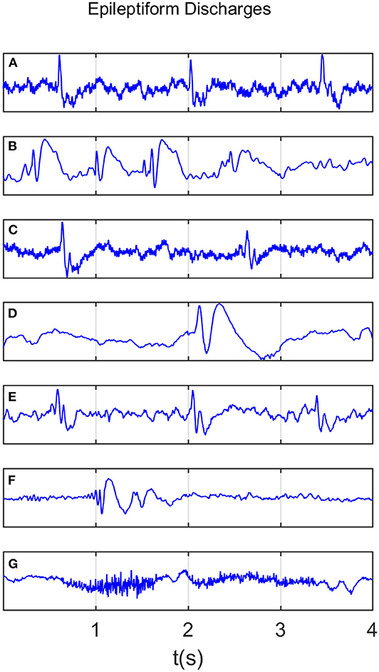
Figure 1. Typical waveforms of the 7 major epileptiform EEG, where (A–G), denotes spike wave, spike and slow wave complex, sharp wave, sharp and slow wave complex, polyspike complex, polyspike and slow wave complex, spike rhythm discharges, respectively.
Recall that a few epileptiform discharge waveforms were considered to simultaneously belong to more than 1 of the 7 different epileptiform discharges. Because of this, further considering the differences among the seven epileptiform discharges becomes impossible and is not pursued here.
2.2. Computation of the Signal Range and the Energy of the Alpha Wave Component
Often EEG epileptic discharges are associated with a larger amplitude than the normal control EEG. This motivates us to compute a simple statistic, which we call Signal Range, to quantify this effect. It is computed as follows:
where x(t) is the EEG signal. This procedure is applied to each of the 19 EEG signals with reference to the earlobes (i.e., the difference of the EEG signals measured at the 19 electrodes and the earlobes), or to the difference of the EEG signals according to the network construction, as detailed in section 2.4. In the former case (i.e., with reference to the earlobe), the final Signal Range is estimated as the average of the 10 largest Signal Range estimated from the 19 EEG signals.
In clinical applications, the brain wave is often categorized into five bands: delta (0.5~3 Hz), theta (4~7 Hz), alpha (8~13 Hz), beta (14~30 Hz), and gamma (>30 Hz), respectively. The alpha wave is most visible when human beings are relaxed with eyes closed. We have found that the alpha wave component on occipital area is often larger for epileptiform discharges. To compute this component, we employ a Fourier transform of the EEG signal, obtain the power spectral density (PSD), and finally integrate the PSD curve over the alpha wave band.
2.3. Adaptive Fractal Analysis (AFA)
AFA utilizes an adaptive detrending algorithm to extract globally smooth trend signals from the data for a given time scale and then analyzes the scaling of the residuals to the fit as a function of the time scale (Hu et al., 2009; Tung et al., 2011). The main steps of AFA to estimate H are as follows:
Suppose starting from a stationary incremental process x(1), x(2), x(3),…, construct a random walk through the following equation:
where is the mean of the process. Based on this random walk u(n), we wish to get a global trend v(i), i = 1, 2, …, N for any specific time scale w, where N is the length of the original time series. This is achieved by dividing the above random walk process into overlapped windows, where the size of each window w contains an odd number of samples, and adjacent windows overlap by (w + 1)/2 samples. The random walk process in each window is fitted by a polynomial of order M, and the polynomials in overlapped regions are combined to yield a single global trend. Typically M should be 1 or 2, a linear or quadratic function. The local fitting ensures that the global trend is optimal or close to optimal, as locally Taylor series expansion is used.
After we get the global trend v(i) of u(i) by the above method, the residual u(i) − v(i) can describe the fluctuation around the global trend. For fractal processes, the Hurst exponent H can be computed by the following equation,
The above equation means by calculating the variance of the residual between the original random walk process and the fitted global trend under a varying window w, we can obtain a linear (or multiple linear) relation between log2 F(w) and log2 w.
To illustrate the procedures described, we have shown in Figure 2A an example of EEG signal and its global smooth trend in Figure 2B. By varying the window size w, we can obtain a curve of log2 F(w) and log2 w shown in Figure 2C, where we observe two scaling regimes, i.e., the curve can be fitted by two straight lines, with the slopes being the Hurst parameter on short and long time scales, respectively. The H on short time scales will be focused here.
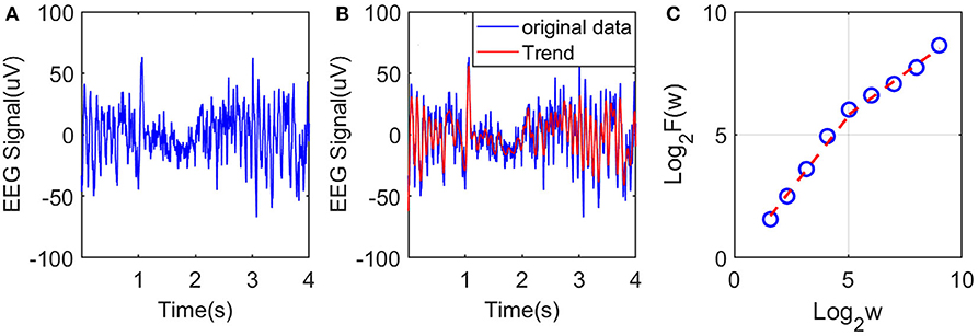
Figure 2. Illustration of estimation of the Hurst exponent using AFA: (A) raw EEG of a channel, (B) fitting (the red curve, with window size w = 21) of the EEG signal by the adaptive algorithm described, and (C) illustration of the scaling law with AFA.
2.4. Cerebral Network Construction
Brain activities involve spatial-temporal coordinated dynamics of numerous neurons in different regions of the brain, i.e., involve numerous functional brain networks. To better characterize the synergistic effects among the brain networks, it is important to construct brain networks based on multi-channel EEG signals. For this purpose, we consider networks with nodes being the 19 electrodes. Between any two of the nodes, we consider the difference between the two associated EEG signals. This is illustrated in Table 1 with a 19 × 19 table consisting of the difference of the EEG signals between two electrodes. Therefore, each element in the Table 1 is a time series. From it we can compute the Signal Range, the relative energy of the alpha wave component, and the Hurst parameter, as detailed earlier. Using each variable, we then obtain a network. Further analysis of these three networks will be based on singular value decomposition (SVD), which we will explain next.
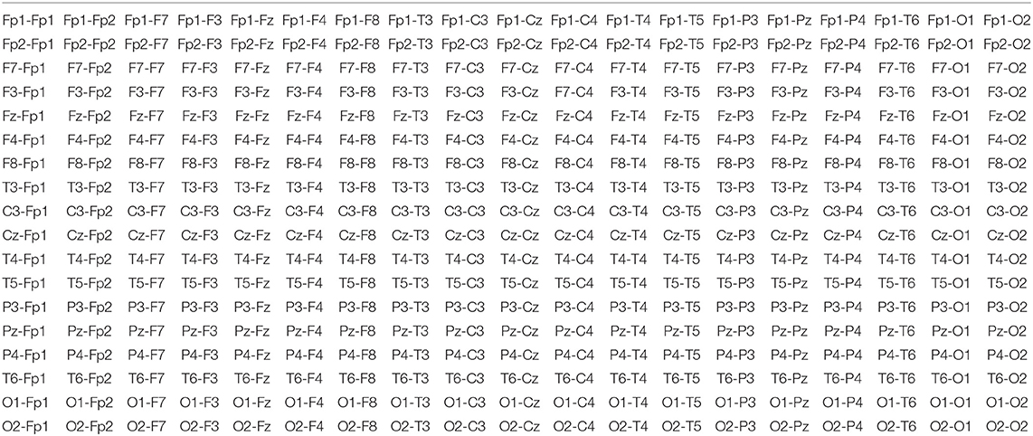
Table 1. A 19 × 19 table consisting of the difference of the EEG signals between two electrodes.
2.5. Singular Value Decomposition (SVD)
SVD is a decomposition method that can be applied to arbitrary matrices. For an n × m matrix A, it is generally expressed as:
where, Un×n and Vm×m are orthogonal matrices, which are composed of eigenvectors of square matrices, AAT and ATA, respectively. Σn×m, called the singular value matrix, is non-zero only on the main diagonal with the elements there being the square root of the eigenvalues of AAT (or ATA). Denote them by Σii = σi, i = 1, 2, …, r, where r is the rank of AAT (or ATA). They are usually written in descending order. In this work, we only need the largest singular value of the three networks based on the Signal Range, the energy of the alpha wave component, and the Hurst parameter.
2.6. Inference of the Localization of the Epileptiform Discharges
Based on the networks constructed using the three variables, the signal range, the relative energy of the alpha wave component, and the Hurst parameter, and using SVD, we can infer the localization of each type of epileptiform discharges. The approach is as follows. For each network of a subject, after we obtain the SVD, we project each column vector of the network to the singular vector corresponding to the largest singular value. The vector is then retained if the absolute value of the projection coefficient is ≥ 0.5. These vectors allow us to determine which channels of the original data are important. The procedure is applied to each of the three networks of the subject. We assume the common channels indicate the localization of this particular type of epileptiform discharge for that subject. As this localization may vary among subjects, we determine the most likely localization of a particular type of epileptiform discharge for all relevant subjects by requiring that each channel occurs at least with certain probability. Here, we has chosen this probability to be 0.55.
2.7. Random Forest Classifier (RF)
Random forest (RF) is an ensemble-based learning technique for classification (Cutler et al., 2012), which has been shown to have high accuracy, is not affected by overtraining, and does not require normalization of the input data. It consists of many separate classification trees, each of which is obtained through a separate bootstrap sample from the data set and each tree classifies the data. A majority vote among the trees provides the final result.
The objective of the RF classifiers used here is to classify which of the two classes an EEG signal belongs to: normal or epileptic discharges. The inputs to the RF classifier are the square of the largest singular values of the three networks (e.g., based on the Signal Range, the energy of the alpha wave component, and Hurst parameters) based on SVD. Following usual practice, we have randomly taken one-third of the total data as testing data and two-thirds of the data for training the model in this paper.
2.8. Evaluation of Performance
To assess the consistency of the diagnosis by the neurologists and machine classification, we need to compute the classification accuracy. This can be accomplished by computing the receiver operating characteristic (ROC) curve and many statistics derived from the ROC curve. In fact, all these are best understand with the confusion matrix, which is a table with two rows and two columns that reports the number of false positives (FP), false negatives (FN), true positives (TP), and true negatives (TN). From them we can define three major metrics:
Note that the sensitivity is also called true positive rate (TPR) and 1 − specificity is also called false positive rate (FPR).
The ROC is a plot of TPR vs. FPR using different threshold values as a sweeping variable. Not suffering from class imbalance, the ROC is a good way to characterize imbalanced data sets. The area below the ROC is called area under curve (AUC). Its value takes from 0 to 1. A value of AUC being 0.5 means the classification model has no predictive ability at all. On the other hand, when the value of AUC reaches 1, it means that the probability density functions of negative and positive classes are completely separated, and the prediction ability is 100%. This is equivalent to the ROC being a unit step function.
3. Results
Recall that among the 640 EEG data sets analyzed here, 69, 82, 174, 72, 64, 77, and 2 data sets are for spike, sharp, spike and slow wave complex, sharp and slow wave complex, polyspike complex, polyspike and slow wave complex, and spike rhythm, respectively, and 100 are for normal controls. Figures 3A,B depicts examples of typical wave forms of epileptiform discharge and the normal EEG. One easy way to appreciate their difference is to construct 2-D phase diagrams shown in Figures 3C,D, which are constructed using the summation of the 19 EEG signals shown in Figures 3A,B. As one can easily understand, the Signal Range can be conveniently estimated from such 2-D phase diagrams. On average, we have observed that the Signal Range is larger for epileptiform discharges than for normal controls. However, this is only in terms of average. Opposite situations also exist. An example is shown in Figure 4, where we observe that the Signal Range for epileptiform discharges can be much smaller than that of normal EEG. Of course, such cases are well-known in the literature and clinically, and motivate us to also account for other features of EEG signals.
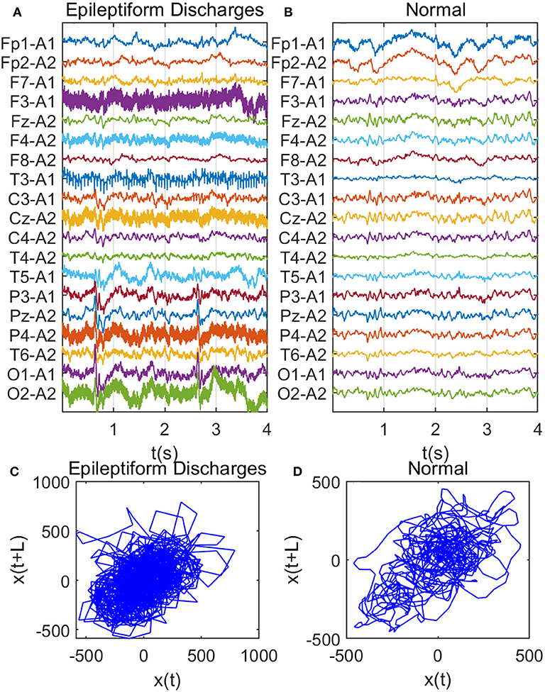
Figure 3. Comparison of epileptiform discharges and normal EEG: (A) example of epileptic discharges, (B) normal EEG, (C,D) 2-D phase diagrams using the summation of the 19 epileptiform discharges and normal EEG signals shown in (A,B), respectively, which can be used to estimate Signal Range.

Figure 4. Same as Figure 3, except data were from another subject showing that Signal Range for epileptiform discharges can be smaller than that of normal EEG: (A) example of epileptic discharges, (B) normal EEG, (C,D) 2-D phase diagrams using the summation of the 19 epileptiform discharges and normal EEG signals shown in (A,B), respectively, which can be used to estimate Signal Range.
To complement the Signal Range, let us examine the long range correlations captured by the Hurst parameter H. We have calculated H for the 19 EEG signals shown in Figures 3, 4 and then taken the average. In Figure 5, we have constructed scatter plots using Signal Range and Hurst parameter H. We observe that the three cases, the polyspike and slow wave complex and the spike rhythm, are completely separated from the normal control group, as shown in Figures 5F,G. The separations for the other 5 cases, although not 100%, are also quite good, as is evident from Figures 5A–E. These plots highly suggest the classification accuracy will be very high.
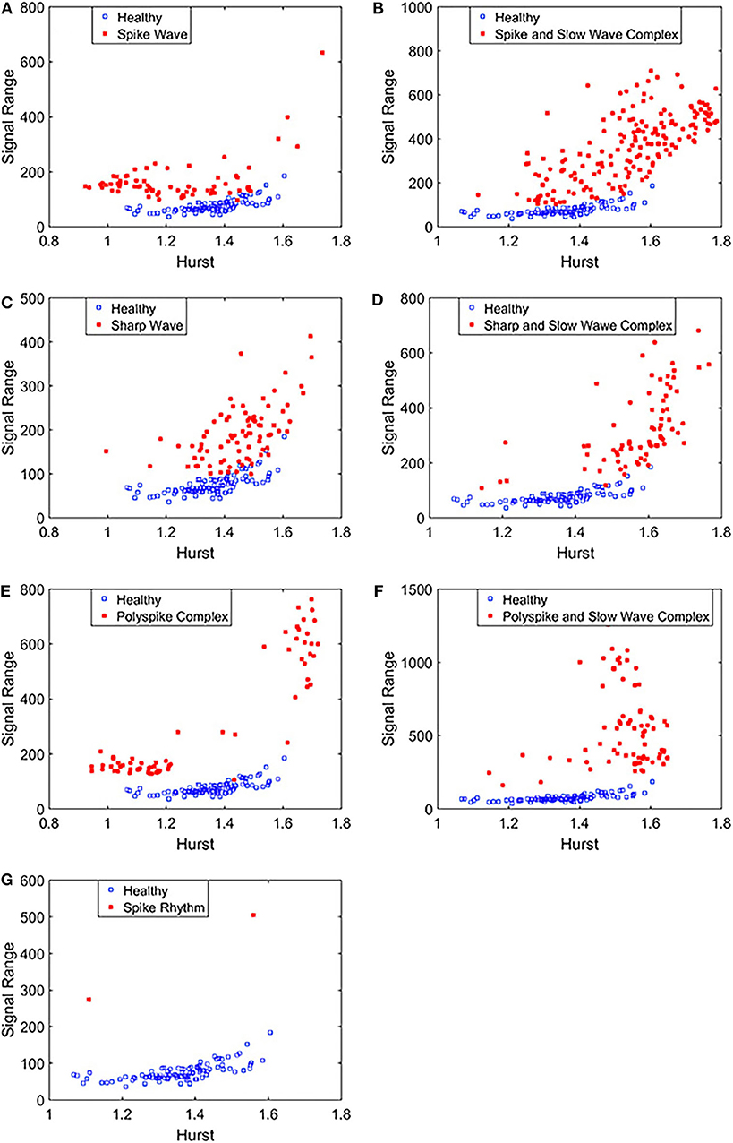
Figure 5. Scatter plots using features Signal Range and the Hurst parameter H, where (A–G), illustrates the different between the seven types of epileptiform discharges (spike wave, spike and slow wave complex, sharp wave, sharp and slow wave complex, polyspike complex, polyspike and slow wave complex, spike rhythm discharges) and normal EEG. These plots highly suggest the classification accuracy will be very high.
To compute the classification accuracy based on the Signal Range and the Hurst parameter, we have employed the RF classifier. We have randomly taken two-thirds of the data as the training data and the remaining one-third of the total data as the testing data. The class distribution of the samples in the training and testing data set is summarized in Table 2. The test performance of the classifier can be determined by computing the metrics defined in section 2.7. The confusion matrix in Table 3 (Method One) shows that 6 out of 34 normal subjects are classified incorrectly by the RF as the epileptiform discharge, 5 out of 180 epileptiform discharges are classified incorrectly as the normal subject. Table 4 shows classification performance. It can be seen that it provides the accuracy of 94.86%, sensitivity and specificity of 97.22 and 82.35%. Figure 6 (the red curve) shows the ROC curve for the testing data of the RF classifier with all seven types of epileptiform discharges grouped into one super class. The AUC of the red curve is 0.9297.
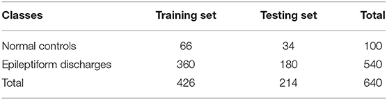
Table 2. Class distribution of the samples in the training and test data sets.
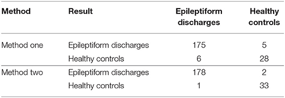
Table 3. Confusion Matrix for the testing data of 180 epileptiform discharges and 34 normal controls: Method One uses Signal Range and H, Method Two is based on the networks constructed from the Signal Range, the energy of the alpha wave component, and the H.
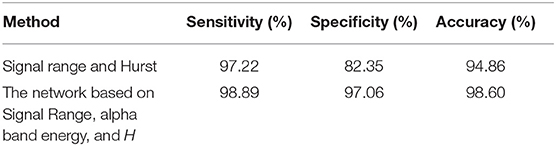
Table 4. Classification performance measures.
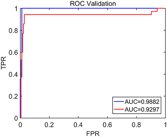
Figure 6. The ROC curve for the testing data. The red and blue curves show respectively the ROC based on methods using Signal Range and H and networks built on Signal Range, energy of the alpha wave component, and H. The AUC for the blue and red curves is 0.9882 and 0.9297, respectively.
To improve the accuracy of classification, we have developed a brain network based approach. Specifically, three separate networks are constructed, based on the Signal Range, the energy of the alpha wave component, and H. Extracting the Signal Range is straightforward. Extracting the energy of the alpha wave component is a little more complicated, but can be readily done (Gao et al., 2007). As shown in Figure 7, we can see that typical PSD for epileptiform discharges and normal EEG show significant difference in the energy of the alpha wave component: it is often larger for epileptiform discharges than for normal. Obtaining H has already been done. Examples of heat maps for these networks are shown in Figure 8. Each of these networks is further analyzed by SVD. We have focused on the square of the first singular value as the final features. In Figure 9, we have constructed scatter plots using the square of the first singular values of the networks based on the Signal Range and the energy of the alpha wave component. We observe that the difference between the seven types of epileptiform discharges and the normal EEG is very significant.
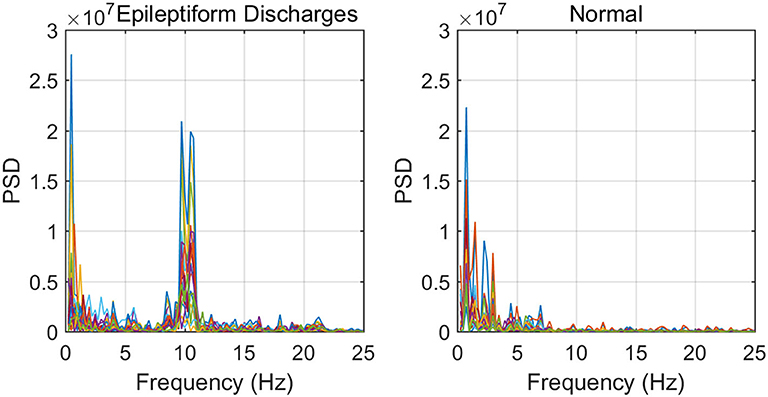
Figure 7. Typical PSD curves for epileptiform discharges and normal EEG showing that the relative energy of the alpha wave component for epileptiform discharges is often larger for that of normal EEGs.
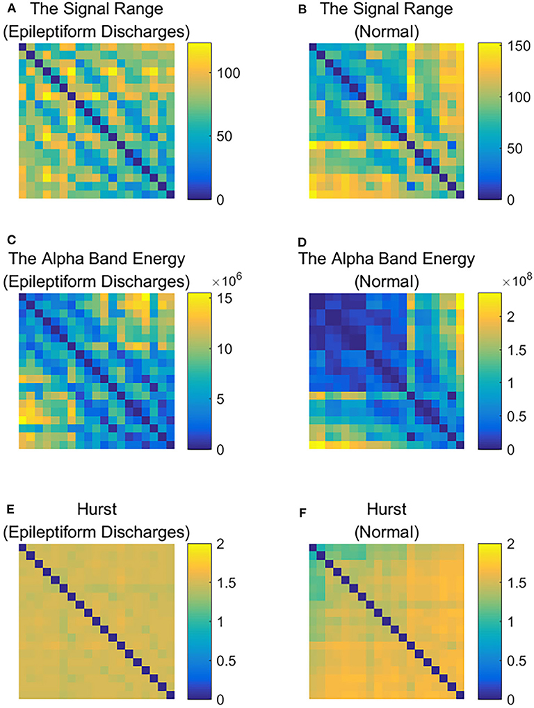
Figure 8. Heat maps illustrating the three types of networks described in section 2: (A,C,E) are for epileptiform discharges while (B,D,F) are for normal EEG.
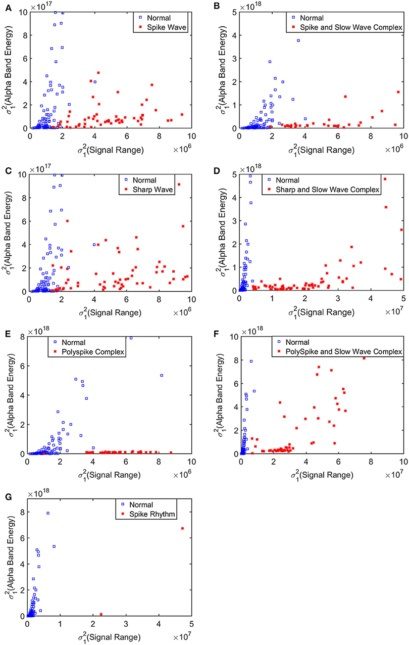
Figure 9. Scatter plots using features from networks based on the Hurst parameter and the Signal Range, where (A–G), illustrates the different between the seven types of epileptiform discharges (spike wave, spike and slow wave complex, sharp wave, sharp and slow wave complex, polyspike complex, polyspike and slow wave complex, spike rhythm discharges) and normal EEG. These plots highly suggest the classification accuracy will be very high.
Again, let us input the square of the first singular values of the networks based on the Signal Range, the energy of the alpha wave component, and the H to the RF classifier. Table 3 (Method Two) shows that 1 out of 34 normal subjects are classified incorrectly as the epileptiform discharge, while 2 out of 180 epileptiform discharge is classified incorrectly as the normal subject. Clearly, this network based method is much improved over the first method, which is based on Signal Range and the Hurst parameter, as the number of misclassifications with this new method is much reduced. With this network based method, the RF classifier has a sensitivity, specificity, and accuracy of 98.89, 97.06, and 98.60%, respectively, in contrast with that of 97.22, 82.35, and 94.86%, which are the basic parameters for the method based on the Signal Range and the Hurst parameter. These numbers are summarized in Table 4, and the blue ROC curve shown in Figure 6 (with all seven types of epileptiform discharges grouped into one super class). While the ROC curve is already close to a unit step function, the result for the training data is even better (and thus not shown here).
We have tried to infer the localizations of each type of epileptiform discharges based on the approach described in section 2.6, whose essence is to equate the sub-network representing the localization of each type of epileptiform discharge to the nodes which generate the most likely alpha band energy, signal range, and the Hurst parameter of that type of epileptiform discharge. The result is shown in Table 5. We observe that while the channels O1 and O2 have appeared in most of the epileptiform discharges, the sub-networks representing the most likely location of each type of epileptiform discharges are different among the seven types of epileptiform discharges studied here.
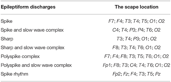
Table 5. The localization of the epileptiform discharges.
Finally, we have compared our results with that of Anh-Dao et al. (2018), who developed an expert system employing multiple state-of-the-art signal processing and machine learning techniques including wavelet transform, spectral filtering, and artificial neural networks for the purpose of automatically detecting epileptic spikes. They achieved an AUC of 0.945, which is slightly better than our Signal Range and the Hurst parameter based method. This is understandable, since our Signal Range and the Hurst parameter based method is so much simpler than their method. Interestingly, our network based approach, which is of similar simplicity with our Signal Range and the Hurst parameter based method, is much more accurate that their method, since our AUC is 0.9882. Most importantly, both of our methods are based on fundamental principles rather than the black-box approach, and therefore, either of our method has the prospect of being widely deployed in clinical setting.
4. Conclusion
In this paper, we have proposed two approaches for distinguishing epileptiform discharges from normal EEGs, with the aim of being able to use them widely in a clinical setting. Our first method is based on Signal Range and the Hurst parameter. Every component of our method can be readily understood and implemented based on first principles. Although simple, the approach already achieves a high detection accuracy of 94.86%. To improve the accuracy of detection, our second method employs the notion of network, with the hope of capturing the functioning of human brain network to some degree. Specifically, our approach involves three types of networks, one based on the Signal Range, the second based on the energy of the alpha wave component of EEG, and the third based on the Hurst parameter. Each of the networks is analyzed by SVD, and the square of the first singular value is utilized to construct features to distinguish epileptiform discharges from normal controls. This network based approach, while still fully first principle based and readily understandable, achieves a very high accuracy of 98.60%. This accuracy is higher than a recent approach proposed by Anh-Dao et al. (2018), which was an expert system employing multiple state-of-the-art signal processing and machine learning techniques including wavelet transform, spectral filtering, and artificial neural networks for the purpose of automatically detecting epileptic spikes. Most importantly, both of our methods are based on fundamental principles rather than the black-box approach, and therefore, are very promising to be used clinically.
We have also designed a network-based approach to infer the localizations of each type of epileptiform discharges based on the networks constructed using the three variables, the signal range, the relative energy of the alpha wave component, and the Hurst parameter. The essence of the approach is to equate the sub-network representing the localization of each type of epileptiform discharge to the nodes which generate the most likely alpha band energy, signal range, and the Hurst parameter of that type of epileptiform discharge. We have found that while the channels O1 and O2 have appeared in most of the epileptiform discharges, the sub-networks representing the most likely location of each type of epileptiform discharges are different among the seven types of epileptiform discharges studied here.
It is worth noting that the epileptiform discharges analyzed here were provided in two batches: in the first batch, which was about 2/3 of the data analyzed here, the accuracy was similar to that reported here. Then more epileptiform data were given to us by clinical doctors to examine whether the accuracy remained as high. It was yes. Nevertheless, the data analyzed here were still quite limited. It would be interesting and important to further validate the proposed approaches with more data in different clinical sets.
Data Availability Statement
The raw data supporting the conclusions of this article will be made available by the authors, without undue reservation.
Ethics Statement
The studies involving human participants were reviewed and approved by the ethics committee of the First Affiliated Hospital to Guangxi Medical University. The participants provided their written informed consent to participate in this study.
Author Contributions
QL performed most of the experimental work. ZZ assisted in data analysis. QH and YW provided the data needed for this experiment and engaged in many analysis and discussions. BX engaged in many discussions. JG conceived the study, provided overall supervision for the study and directed all phases of the study and including writing of the manuscript. All authors read and approved the final manuscript.
Funding
This research was supported by the National Natural Science Foundation of China under Grant Nos. 71661002 and 41671532, and by the Fundamental Research Funds for the Central Universities. One of the authors (JG) also benefited tremendously from participating the long program on culture analytics organized by the Institute for Pure and Applied Mathematics (IPAM) at UCLA, which is supported by the National Science Foundation.
Conflict of Interest
The authors declare that the research was conducted in the absence of any commercial or financial relationships that could be construed as a potential conflict of interest.
References
Acharya, J. N., and Acharya, V. J. (2019). Overview of EEG montages and principles of localization. J. Clin. Neurophysiol. 36, 325–329. doi: 10.1097/WNP.0000000000000538
Adeli, H., Zhou, Z., and Dadmehr, N. (2003). Analysis of EEG records in an epileptic patient using wavelet transform. J. Neurosci. Methods 123, 69–87. doi: 10.1016/S0165-0270(02)00340-0
Anh-Dao, N. T., Linh-Trung, N., Van Nguyen, L., Tran-Duc, T., Boashash, B., et al. (2018). A multistage system for automatic detection of epileptic spikes. Rev. J. Electron. Commun. 8, 1–12. doi: 10.21553/rev-jec.166
Antoniades, A., Spyrou, L., Took, C. C., and Sanei, S. (2016). “Deep learning for epileptic intracranial EEG data,” in 2016 IEEE 26th International Workshop on Machine Learning for Signal Processing (MLSP) (Vietri Sul Mare: IEEE), 1–6. doi: 10.1109/MLSP.2016.7738824
Arunkumar, N., Ram Kumar, K., and Venkataraman, V. (2016). Automatic detection of epileptic seizures using permutation entropy, tsallis entropy and kolmogorov complexity. J. Med. Imaging Health Inform. 6, 526–531. doi: 10.1166/jmihi.2016.1710
Arunkumar, N., Ramkumar, K., Venkatraman, V., Abdulhay, E., Fernandes, S. L., Kadry, S., et al. (2017). Classification of focal and non focal EEG using entropies. Pattern Recogn. Lett. 94, 112–117. doi: 10.1016/j.patrec.2017.05.007
Bartsch, R. P., Liu, K. K., Bashan, A., and Ivanov, P. C. (2015). Network physiology: how organ systems dynamically interact. PLoS ONE 10:e142143. doi: 10.1371/journal.pone.0142143
Bashan, A., Bartsch, R. P., Kantelhardt, J. W., Havlin, S., and Ivanov, P. C. (2012). Network physiology reveals relations between network topology and physiological function. Nat. Commun. 3, 1–9. doi: 10.1038/ncomms1705
Basiri, R., Shariatzadeh, A., Wiebe, S., and Aghakhani, Y. (2019). Focal epilepsy without interictal spikes on scalp EEG: a common finding of uncertain significance. Epilepsy Res. 150, 1–6. doi: 10.1016/j.eplepsyres.2018.12.009
Brienza, M., Davassi, C., and Mecarelli, O. (2019). “Artifacts,” in: Clinical Electroencephalography, ed O. Mecarelli (Cham: Springer), 109–130. doi: 10.1007/978-3-030-04573-9_8
Chen, D., Wan, S., Xiang, J., and Bao, F. S. (2017). A high-performance seizure detection algorithm based on discrete wavelet transform (DWT) and EEG. PLoS ONE 12:e173138. doi: 10.1371/journal.pone.0173138
Chen, Z., Hu, K., Carpena, P., Bernaola-Galvan, P., Stanley, H. E., and Ivanov, P. C. (2005). Effect of nonlinear filters on detrended fluctuation analysis. Phys. Rev. E 71:011104. doi: 10.1103/PhysRevE.71.011104
Chen, Z., Ivanov, P. C., Hu, K., and Stanley, H. E. (2002). Effect of nonstationarities on detrended fluctuation analysis. Phys. Rev. E 65:041107. doi: 10.1103/PhysRevE.65.041107
Christodoulakis, M., Hadjipapas, A., Papathanasiou, E. S., Anastasiadou, M., Papacostas, S. S., and Mitsis, G.D. (2013). “Graph-theoretic analysis of scalp eeg brain networks in epilepsy-the influence of montage and volume conduction,” in: 13th IEEE International Conference on BioInformatics and BioEngineering (Chania), 1–4. doi: 10.1109/BIBE.2013.6701572
Cutler, A., Cutler, D. R., and Stevens, J.R. (2012). “Random Forests,” in: Ensemble Machine Learning, eds C. Zhang and Y. Q. Ma (Boston, MA: Springer), 157–175. doi: 10.1007/978-1-4419-9326-7_5
Denéve, S., Alemi, A., and Bourdoukan, R. (2017). The brain as an efficient and robust adaptive learner. Neuron 94, 969–977. doi: 10.1016/j.neuron.2017.05.016
Faust, O., Acharya, U. R., Adeli, H., and Adeli, A. (2015). Wavelet-based EEG processing for computer-aided seizure detection and epilepsy diagnosis. Seizure 26, 56–64. doi: 10.1016/j.seizure.2015.01.012
Gao, J., Cao, Y., Tung, W.-W., and Hu, J. (2007). Multiscale Analysis of Complex Time Series: Integration of Chaos and Random Fractal Theory, and Beyond. Hoboken, NJ: John Wiley & Sons. doi: 10.1002/9780470191651
Gao, J., Hu, J., Mao, X., and Perc, M. (2012a). Culturomics meets random fractal theory: insights into long-range correlations of social and natural phenomena over the past two centuries. J. R. Soc. Interface 9, 1956–1964. doi: 10.1098/rsif.2011.0846
Gao, J., Hu, J., and Tung, W.-W. (2011a). Complexity measures of brain wave dynamics. Cogn. Neurodyn. 5, 171–182. doi: 10.1007/s11571-011-9151-3
Gao, J., Hu, J., and Tung, W.-W. (2011b). Facilitating joint chaos and fractal analysis of biosignals through nonlinear adaptive filtering. PLoS ONE 6:e24331. doi: 10.1371/journal.pone.0024331
Gao, J., Hu, J., and Tung, W.-w. (2012b). Entropy measures for biological signal analyses. Nonlin. Dyn. 68, 431–444. doi: 10.1007/s11071-011-0281-2
Geier, C., and Lehnertz, K. (2017). Which brain regions are important for seizure dynamics in epileptic networks? Influence of link identification and EEG recording montage on node centralities. Int. J. Neural Syst. 27:1650033. doi: 10.1142/S0129065716500337
Gupta, G., Pequito, S., and Bogdan, P. (2018). “Dealing with unknown unknowns: Identification and selection of minimal sensing for fractional dynamics with unknown inputs,” in: 2018 Annual American Control Conference (ACC) (Milwaukee, WI), 2814–2820. doi: 10.23919/ACC.2018.8430866
Gupta, G., Pequito, S., and Bogdan, P. (2019). “Learning latent fractional dynamics with unknown unknowns,” in: 2019 American Control Conference (ACC) (Philadelphia, PA), 217–222. doi: 10.23919/ACC.2019.8815074
Haufe, S., DeGuzman, P., Henin, S., Arcaro, M., Honey, C. J., Hasson, U., et al. (2018). Reliability and correlation of fMRI, ECOG and EEG during natural stimulus processing. BioRxiv 2018:207456. doi: 10.1101/207456
Hu, J., Gao, J., and Wang, X. (2009). Multifractal analysis of sunspot time series: the effects of the 11-year cycle and fourier truncation. J. Stat. Mech. 2009:P02066. doi: 10.1088/1742-5468/2009/02/P02066
Hu, K., Ivanov, P. C., Chen, Z., Carpena, P., and Stanley, H. E. (2001). Effect of trends on detrended fluctuation analysis. Phys. Rev. E 64:011114. doi: 10.1103/PhysRevE.64.011114
Islam, M. K., Rastegarnia, A., and Yang, Z. (2016). Methods for artifact detection and removal from scalp EEG: a review. Neurophysiol. Clin. 46, 287–305. doi: 10.1016/j.neucli.2016.07.002
Ivanov, P. C., Liu, K. K., and Bartsch, R. P. (2016). Focus on the emerging new fields of network physiology and network medicine. New J. Phys. 18:100201. doi: 10.1088/1367-2630/18/10/100201
Kane, N., Acharya, J., Benickzy, S., Caboclo, L., Finnigan, S., Kaplan, P. W., et al. (2017). A revised glossary of terms most commonly used by clinical electroencephalographers and updated proposal for the report format of the EEG findings. Revision 2017. Clin. Neurophysiol. Pract. 2:170. doi: 10.1016/j.cnp.2017.07.002
Kappel, S. L., Looney, D., Mandic, D. P., and Kidmose, P. (2017). Physiological artifacts in scalp EEG and ear-EEG. Biomed. Eng. Online 16:103. doi: 10.1186/s12938-017-0391-2
Kuswanto, H., Salamah, M., and Fachruddin, M. I. (2017). Random forest classification and support vector machine for detecting epilepsyusing electroencephalograph records. Am. J. Appl. Sci. 14, 533–539. doi: 10.3844/ajassp.2017.533.539
Kuznetsov, N., Bonnette, S., Gao, J., and Riley, M. A. (2013). Adaptive fractal analysis reveals limits to fractal scaling in center of pressure trajectories. Ann. Biomed. Eng. 41, 1646–1660. doi: 10.1007/s10439-012-0646-9
Li, F., Liang, Y., Zhang, L., Yi, C., Liao, Y., Jiang, Y., et al. (2019). Transition of brain networks from an interictal to a preictal state preceding a seizure revealed by scalp EEG network analysis. Cogn. Neurodyn. 13, 175–181. doi: 10.1007/s11571-018-09517-6
Liu, K. K., Bartsch, R. P., Ma, Q. D., and Ivanov, P. C. (2015). Major component analysis of dynamic networks of physiologic organ interactions. J. Phys. 640:012013. doi: 10.1088/1742-6596/640/1/012013
Lopez, S., Gross, A., Yang, S., Golmohammadi, M., Obeid, I., and Picone, J. (2016). “An analysis of two common reference points for EEGs,” in: 2016 IEEE Signal Processing in Medicine and Biology Symposium (SPMB) (Philadelphia, PA), 1–5. doi: 10.1109/SPMB.2016.7846854
Ma, Q. D., Bartsch, R. P., Bernaola-Galván, P., Yoneyama, M., and Ivanov, P. C. (2010). Effect of extreme data loss on long-range correlated and anticorrelated signals quantified by detrended fluctuation analysis. Phys. Rev. E 81:031101. doi: 10.1103/PhysRevE.81.031101
Martis, R. J., Tan, J. H., Chua, C. K., Loon, T. C., Yeo, S. W. J., and Tong, L. (2015). Epileptic EEG classification using nonlinear parameters on different frequency bands. J. Mech. Med. Biol. 15:1550040. doi: 10.1142/S0219519415500402
Medvedeva, T. M., Lüttjohann, A., van Luijtelaar, G., and Sysoev, I. V. (2016). “Evaluation of nonlinear properties of epileptic activity using largest lyapunov exponent,” in: Saratov Fall Meeting 2015: Third International Symposium on Optics and Biophotonics and Seventh Finnish-Russian Photonics and Laser Symposium (PALS), Vol. 9917, (Saratov: International Society for Optics and Photonics), 991724.
Mirowski, P. W., LeCun, Y., Madhavan, D., and Kuzniecky, R. (2008). “Comparing svm and convolutional networks for epileptic seizure prediction from intracranial EEG,” in: 2008 IEEE Workshop on Machine Learning for Signal Processing (Cancun), 244–249. doi: 10.1109/MLSP.2008.4685487
Nicolaou, N., and Georgiou, J. (2012). Detection of epileptic electroencephalogram based on permutation entropy and support vector machines. Expert Syst. Appl. 39, 202–209. doi: 10.1016/j.eswa.2011.07.008
Pardey, J., Roberts, S., and Tarassenko, L. (1996). A review of parametric modelling techniques for EEG analysis. Med. Eng. Phys. 18, 2–11. doi: 10.1016/1350-4533(95)00024-0
Peng, C., Buldyrev, S., Havlin, S., Simons, M., Stanley, H., and Golberger, A. (1994). Scaling features of noncoding DNA. Phys. Rev. E 49, 1685–1689. doi: 10.1103/PhysRevE.49.1685
Perkins, A. (2019). Epilepsy: an electrical storm in the brain. Nurs. Made Incred. Easy 17, 42–50. doi: 10.1097/01.NME.0000559583.43254.ab
Pratiher, S., Patra, S., and Bhattacharya, P. (2016). “On the marriage of kolmogorov complexity and multi-fractal parameters for epileptic seizure classification,” in: 2016 2nd International Conference on Contemporary Computing and Informatics (IC3I) (Noida), 831–836. doi: 10.1109/IC3I.2016.7918797
Rana, A. Q., Ghouse, A. T., and Govindarajan, R. (2017). “Basics of electroencephalography (EEG),” in: Neurophysiology in Clinical Practice, ed J. Renwick (Cham: Springer), 3–9. doi: 10.1007/978-3-319-39342-1_1
Richards, J. B., Barker, L., Husain, A. M., Luedke, M., Sinha, S. R., and Zafar, M. (2018). S11. EEG source localization of interictal discharges and outcome for litt for temporal lobe epilepsy. Clin. Neurophysiol. 129:e146. doi: 10.1016/j.clinph.2018.04.371
Riley, M. A., Bonnette, S., Kuznetsov, N., Wallot, S., and Gao, J. (2012). A tutorial introduction to adaptive fractal analysis. Front. Physiol. 3:371. doi: 10.3389/fphys.2012.00371
Rios, W. A., Olguín, P. V., Mena, D. A., Cabrera, M. C., Escalona, J., Garcia, A. M., et al. (2019). The influence of EEG references on the analysis of spatio-temporal interrelation patterns. Front. Neurosci. 13:941. doi: 10.3389/fnins.2019.00941
Seeck, M., Koessler, L., Bast, T., Leijten, F., Michel, C., Baumgartner, C., et al. (2017). The standardized EEG electrode array of the IFCN. Clin. Neurophysiol. 128, 2070–2077. doi: 10.1016/j.clinph.2017.06.254
Sharmila, A., and Geethanjali, P. (2019). A review on the pattern detection methods for epilepsy seizure detection from EEG signals. Biomed. Eng. 64, 507–517. doi: 10.1515/bmt-2017-0233
Shen, T.-W., Kuo, X., and Hsin, Y.-L. (2009). “Ant k-means clustering method on epileptic spike detection,” in: 2009 Fifth International Conference on Natural Computation, Vol. 6 (Tianjin), 334–338. doi: 10.1109/ICNC.2009.639
Sikdar, D., Roy, R., and Mahadevappa, M. (2018). Epilepsy and seizure characterisation by multifractal analysis of EEG subbands. Biomed. Signal Process. Control 41, 264–270. doi: 10.1016/j.bspc.2017.12.006
Smith, K., and Escudero, J. (2017). The complex hierarchical topology of EEG functional connectivity. J. Neurosci. Methods 276, 1–12. doi: 10.1016/j.jneumeth.2016.11.003
Smitha, K., Akhil Raja, K., Arun, K., Rajesh, P., Thomas, B., Kapilamoorthy, T., et al. (2017). Resting state fMRI: a review on methods in resting state connectivity analysis and resting state networks. Neuroradiol. J. 30, 305–317. doi: 10.1177/1971400917697342
Subasi, A. (2007). EEG signal classification using wavelet feature extraction and a mixture of expert model. Expert Syst. Appl. 32, 1084–1093. doi: 10.1016/j.eswa.2006.02.005
Subasi, A., Kevric, J., and Canbaz, M. A. (2019). Epileptic seizure detection using hybrid machine learning methods. Neural Comput. Appl. 31, 317–325. doi: 10.1007/s00521-017-3003-y
Tautan, A. M., Munteanu, A. I., Taralunga, D. D., Strungaru, R., and Ungureanu, G. M. (2018). “Automated classification of epileptiform discharges in EEG signals using the wavelet transform,” in: 2018 International Conference and Exposition on Electrical And Power Engineering (EPE), (Lasi), 0877–0882. doi: 10.1109/ICEPE.2018.8559773
Toet, M. C., Groenendaal, F., Osredkar, D., van Huffelen, A. C., and de Vries, L. S. (2005). Postneonatal epilepsy following amplitude-integrated EEG-detected neonatal seizures. Pediatr. Neurol. 32, 241–247. doi: 10.1016/j.pediatrneurol.2004.11.005
Tung, W.-W., Gao, J., Hu, J., and Yang, L. (2011). Detecting chaos in heavy-noise environments. Phys. Rev. E 83:046210. doi: 10.1103/PhysRevE.83.046210
Ullah, I., Hussain, M., Aboalsamh, H., et al. (2018). An automated system for epilepsy detection using EEG brain signals based on deep learning approach. Expert Syst. Appl. 107, 61–71. doi: 10.1016/j.eswa.2018.04.021
van Putten, M. J., de Carvalho, R., and Tjepkema-Cloostermans, M. C. (2018). F85. deep learning for detection of epileptiform discharges from scalp EEG recordings. Clin. Neurophysiol. 129, e98-e99. doi: 10.1016/j.clinph.2018.04.248
Vanherpe, P., and Schrooten, M. (2017). Minimal eeg montage with high yield for the detection of status epilepticus in the setting of postanoxic brain damage. Acta Neurol. Belgica 117, 145–152. doi: 10.1007/s13760-016-0663-9
Wang, J., Khosrowabadi, R., Ng, K.-K., Hong, Z., Chong, J. S. X., Wang, Y., et al. (2018). Alternations in brain network topology and structural-functional connectome coupling relate to cognitive impairment. Front. Aging Neurosci. 10:404. doi: 10.3389/fnagi.2018.00404
Wang, Q., Valdés-Hernández, P. A., Paz-Linares, D., Bosch-Bayard, J., Oosugi, N., Komatsu, M., et al. (2019). EECog-Comp: An open source platform for concurrent EEG/ECoGcomparisons-applications to connectivity studies. Brain Topogr. 32, 1–19. doi: 10.1007/s10548-019-00708-w
Xu, L., Ivanov, P. C., Hu, K., Chen, Z., Carbone, A., and Stanley, H. E. (2005). Quantifying signals with power-law correlations: a comparative study of detrended fluctuation analysis and detrended moving average techniques. Phys. Rev. E 71:051101. doi: 10.1103/PhysRevE.71.051101
Xu, Y., Ma, Q. D., Schmitt, D. T., Bernaola-Galván, P., and Ivanov, P. C. (2011). Effects of coarse-graining on the scaling behavior of long-range correlated and anti-correlated signals. Phys. A 390, 4057–4072. doi: 10.1016/j.physa.2011.05.015
Xue, Y., and Bogdan, P. (2017). Reliable multi-fractal characterization of weighted complex networks: algorithms and implications. Sci. Rep. 7, 1–22. doi: 10.1038/s41598-017-07209-5
Keywords: EEG, epileptiform discharges, adaptive fractal analysis, Hurst parameter, singular value decomposition, brain network
Citation: Li Q, Gao J, Zhang Z, Huang Q, Wu Y and Xu B (2020) Distinguishing Epileptiform Discharges From Normal Electroencephalograms Using Adaptive Fractal and Network Analysis: A Clinical Perspective. Front. Physiol. 11:828. doi: 10.3389/fphys.2020.00828
Received: 26 March 2020; Accepted: 22 June 2020;
Published: 05 August 2020.
Edited by:
Plamen Ch. Ivanov, Boston University, United StatesReviewed by:
Marina De Tommaso, University of Bari Aldo Moro, ItalyPaul Bogdan, University of Southern California, Los Angeles, United States
Rudolf Marcel Füchslin, Zurich University of Applied Sciences, Switzerland
Copyright © 2020 Li, Gao, Zhang, Huang, Wu and Xu. This is an open-access article distributed under the terms of the Creative Commons Attribution License (CC BY). The use, distribution or reproduction in other forums is permitted, provided the original author(s) and the copyright owner(s) are credited and that the original publication in this journal is cited, in accordance with accepted academic practice. No use, distribution or reproduction is permitted which does not comply with these terms.
*Correspondence: Jianbo Gao, amJnYW8ucG1iQGdtYWlsLmNvbQ==; Yuan Wu, d3V5dWFuOTBAMTI2LmNvbQ==