Application of Radon Transform to Multi-Angle Measurements Made by the Research Scanning Polarimeter: A New Approach to Cloud Tomography. Part I: Theory and Tests on Simulated Data

1 Introduction

Tomography is a retrieval technique inverting a 2D spatial density from a dataset of measured “slices” (τoμoς, tomos means “slice” in Greek), which are the integrals of this density over transect lines (chords). The collection of slices parameterized by angle and offset of the chords (relative a selected central point) constitutes a 2D dataset called tomogram (or “ray sum” in medicine). The original 2D density can be restored back from its tomogram using the inverse Radon transform, introduced in 1917 by Austrian mathematician Johann Radon (Radon, 1917; Radon and Parks, 1986). This transform serves as the mathematical basis for the X-ray tomography (commonly known as the CT scan in medicine, with “CT” referring to “computer tomography”).

While topography is an analysis of essentially active measurements (when a ray sent through the object is captured by a detector on its other side), this term sometimes is used in cloud remote sensing in a wider sense: as any technique of inversion of cloud interior structure from remote optical measurements. Previously developed retrieval algorithms of this kind (e.g., Martin and Hasekamp, 2018; Levis et al., 2020) rely on least-square-fit (LSF) inversions in highly-multi-dimensional space of possible cloud configurations and use extensive 3D RT computations on each iterative step. Levis et al. (2020) call such algorithms “passive tomography” using the word “tomography” in that wider sense (while “slice” measurements or Radon transform may not be necessarily used). Below we will use this definition when addressing LSF techniques as well as our own.

We present a new algorithm for inversion of the internal cloud structure. It is ideologically closer than LSF approaches to “tomography” in the traditional sense, while also relying on passive optical measurements. Such measurements obviously cannot directly provide a proper tomogram (directional optical thickness as a function of angle and offset of the viewing ray), but allow for estimation of it using a nested family of “cloud shapes” corresponding to an array of thresholds in the measured total reflectance. Once such tomogram is obtained, we proceed following the standard tomographic procedure and apply inverse Radon transform to it deriving a 2D field of the extinction coefficients (which requires calibration using independent measurements). So this technique may be called “semi-tomographic”. Note that unlike the LSF techniques, our method does not require iterative 3D RT computations, but relies on a number of empirical assumptions which we validate using simulated data. In fact, we only use simulated data (LES + 3D RT) for testing of our algorithm and for selection of an appropriate “proxy” formula relating the measured reflectance to the corresponding directional COT.

The presented algorithm has been developed for the Research Scanning Polarimeter (RSP) measurements. The RSP (Cairns et al., 1999) is an airborne sensor which high-resolution along-track scanning provides sufficient number of view rays to constrain cloud shapes (Alexandrov et al., 2016a) and also to derive droplet size distribution (DSD) profiles along the cloud side (Alexandrov et al., 2020). The RSP served as a prototype for the satellite Aerosol Polarimetery Sensor (APS) built for the NASA Glory Project (Mishchenko et al., 2006; Mishchenko et al., 2007). Currently the cloud retrieval algorithms developed for the RSP are being adopted for use with the measurements of the spaceborne polarimeters on the upcoming Plankton, Aerosol, Cloud Ocean Ecosystem (PACE) satellite mission (Werdell et al., 2019). During the past decades the RSP has been deployed during numerous NASA field campaigns (see e.g., Alexandrov et al., 2015; Alexandrov et al., 2016a; Alexandrov et al., 2016b; Sinclair et al., 2017; Alexandrov et al., 2018; Sinclair et al., 2019).

This study was inspired by the RSP measurements made during NASA’s Cloud, Aerosol and Monsoon Processes Philippines Experiment (CAMP²Ex) conducted in 2019. This campaign took place off Philippines coast during the monsoon season, which is characterized by abundance of moisture and strong convections producing wide variety of cloud types and shapes which present interesting cases for application of our tomographic analysis. We will report analyses of the actual RSP data from CAMP²Ex in subsequent publications following this paper.

2 The Research Scanning Polarimeter Measurements and Retrievals

The RSP has high angular resolution of 14 mrad field of view (FOV) with measurements made at 0.8° intervals within ±60° from nadir. The translation of these parmeters into spatial resolutions of the RSP datasets depends on the speed and the altitude of the aircraft (Alexandrov et al., 2016a) and can range from about 200 m for high-altitude NASA ER-2 down to less than 100 m for more conventional NASA airplanes (P3-B, B-200, UC-12, C-130) which fly slower and at lower altitude.

The RSP measures both total and polarized reflectances in nine spectral channels. Its measurement geometry and the view-line aggregation types used for different kinds of retrievals are schematically presented in Figure 1. The polarized reflectances in the rainbow (cloud bow) scattering range (135°–165°) have been routinely used for retrieval of droplet size distributions in liquid-water clouds (Alexandrov et al., 2012a; Alexandrov et al., 2012b).

FIGURE 1

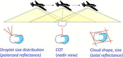
FIGURE 1. Schematic representation of the RSP’s measurement geometry (top) and the view-line aggregations used for different types of retrievals (bottom).

The COT retrievals from RSP-measured total reflectances at nadir view are made using a modification of the legacy bi-spectral technique (Nakajima and King, 1990). In the modified algorithm no absorbing spectral channels are used. Instead, the droplet effective radius is retrieved from the polarized reflectance (Alexandrov et al., 2012a) and used to derive the COT value from the look-up table (LUT) computed for non-absorbing 863 nm channel. This LUT was built using plain-parallel radiative transfer computations, thus, this method can produce biases in COT values in the presence of 3D radiative effects (such as light escape from broken cloud’s sides or shadowing at low Sun angles).

The standard operational RSP cloud top height (CTH) product is based on a stereo block-correlation algorithm developed by A. Wasilewski. This technique has been generalized to multi-layer cloud scenes by Sinclair et al. (2017).

3 The Simulated Dataset

For illustration and validation of the proposed tomographic technique we use simulated RSP measurements generated by the 3D radiative transfer (RT) model called “Monte Carlo code for the phYSically correct Tracing of photons In Cloudy atmospheres” (MYSTIC Mayer, 2009; Emde et al., 2010) applied to a LES dataset with 100 m horizontal and 40 m vertical resolution. This dataset is an idealized representation of the shallow, maritime convection cloud fields (Ackerman et al., 2004) observed during the Rain in Cumulus over the Ocean project (RICO van Zanten et al., 2011). In the 3D RT computations the actual bin-by-bin LES DSDs were replaced by gamma distributions with the same effective radius as in the microphysical model, while the effective variance was uniformly set to 0.1 throughout the cloud (see Hansen and Travis, 1974; Alexandrov et al., 2018 for definitions). In this simulation the virtual RSP makes measurements at 555 nm wavelength and is assumed to fly in the solar principal plane (corresponding to the y-axis of the LES grid) at 2.4 km altitude. The solar zenith angle is set to 40° and the surface albedo—to 5%. These simulations have been already used in our previous work (Alexandrov et al., 2010; Alexandrov et al., 2012a; Alexandrov et al., 2016a).

We selected the last (No. 3) cloud from the segment used in Alexandrov et al. (2016a). Figure 2A presents the distribution of the droplet number concentration N_c (measured in cm⁻³) within the 2D cross section of this cloud. Figure 2B shows the corresponding field of the effective radius r_eff (measured in μm) of the droplet size distribution, this plot is restricted to the area with N_c ≥ 10 cm⁻³ for consistency with Figure 2A. The effective variance v_eff in the RT model is constant and set to 0.1. The effective radius and variance of cloud droplet DSD are routinely retrieved from the RSP measurements of the polarized reflectance using the parametric algorithm (Alexandrov et al., 2012a).

FIGURE 2

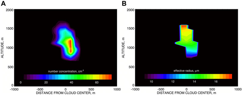
FIGURE 2. (A) droplet number concentration field in the 2D cross section of the LES-generated Cu cloud to be used in this study. (B) same as (A) but for the effective radius of the droplet size distribution. The plot is restricted to the area with N_c ≥ 10 cm⁻³.

The extinction coefficient field for the 2D cross section of this cloud is presented in Figure 4A. It is derived from the cloud microphysical parameters using the following formula

$k_{\mathrm{e}\mathrm{x}\mathrm{t}}=Q_{\mathrm{e}\mathrm{x}\mathrm{t}}{N}_c\pi ⟨r^2⟩\times 10^{-6},(1)$

where N_c is the droplet number concentration (in cm⁻³), r is the droplet radius (in μm), and Q_ext is the extinction efficiency (Hansen and Travis, 1974). The factor 10^–6 makes the units of k_ext to be m⁻¹. However, for our purposes we can use a simplified version of Eq. 1

$k_{\mathrm{e}\mathrm{x}\mathrm{t}}\approx 2\pi N_c{r}_{\mathrm{e}\mathrm{ff}}^2\left(1-v_{\mathrm{e}\mathrm{ff}}\right)\left(1-2v_{\mathrm{e}\mathrm{ff}}\right)\times 10^{-6},(2)$

where we have assumed that Q_ext ≈ 2 for large cloud droplets and expressed the second moment ⟨r²⟩ of the droplet size distribution in terms of r_eff and v_eff [assuming that the DSD has gamma-distribution shape (Hansen and Travis, 1974)].

4 Radon Transform

In this study we use the implementation of the Radon transform from the standard Interactive Data Language (IDL v.8.4) library (RADON function) with ramp filter added. The 2D field to be determined is the spatial distribution of the cloud extinction coefficient k_ext (x, y) (measured in m⁻¹), whose integral over a linear transect (chord) through the cloud yields the directional COT

${\tau }_{\mathrm{d}}\left(\psi ,\rho \right)=\underset{-\infty }{\overset{\infty }{\int }}{k}_{\mathrm{e}\mathrm{x}\mathrm{t}}\left(\rho \cos \psi -s\sin \psi ,\rho \sin \psi +s\cos \psi \right)\mathrm{d}s,(3)$

where s is the distance along the chord. The geometric setup of the method is schematically shown in Figure 3A. The resulting value of the directional COT is attributed to a point in the tomogram (the Radon space) with the coordinates (ψ, ρ) as depicted in Figure 3B.

FIGURE 3

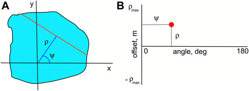
FIGURE 3. Radon transform geometry: (A) in the physical space the extinction coefficient (light blue) is integrated along the chord (red) parameterized by the angle ψ and the offset ρ in order to get the directional COT τ_d (ψ, ρ); (B) the representation (red dot) of the location where this chord’s value τ_d (ψ, ρ) is placed in the Radon’s tomogram.

The inverse Radon transform deriving the extinction coefficient distribution from the tomogram is called “filtered backprojection.” It consists of two parts. First, the ramp filter is applied to the tomogram τ_d (ψ, ρ) in ρ-direction transforming it into its filtered version

${\tilde{\tau }}_{\mathrm{d}}\left(\psi ,\rho \right)={\mathrm{F}\mathrm{F}\mathrm{T}}^{-1}\left[|f|\cdot {\widehat{\tau }}_{\mathrm{d}}\left(\psi ,f\right)\right],(4)$

where

${\widehat{\tau }}_{\mathrm{d}}\left(\psi ,f\right)={\mathrm{F}\mathrm{F}\mathrm{T}}_{\rho }\left[{\tau }_{\mathrm{d}}\left(\psi ,\rho \right)\right].(5)$

Here f is frquency and FFT is the Fast Fourier Transform operator (implemented in IDL by the function FFT). The ramp filter is a high pass filter with V-shaped kernel |f| in frequency domain. It prevents low-frequency blurring of the image. While filtering is an important part of the algorithm, it, unfortunately, has been omitted in the IDL v.8.4 distribution, so we designed our own version.

After filtering the backprojection itself is applied yielding the inverted extinction field:

$k_{\mathrm{e}\mathrm{x}\mathrm{t}}^{\prime }\left(x,y\right)=\underset{0}{\overset{\pi }{\int }}{\tilde{\tau }}_{\mathrm{d}}\left(\psi ,x\cos \psi +y\sin \psi \right)\mathrm{d}\psi .(6)$

Note that inverse Radon transform is not exact, so the inverted $k_{\mathrm{e}\mathrm{x}\mathrm{t}}^{\prime }(x,y)$ may be somehow spatially different in structure from the original k_ext (x, y). The inversion is also defined up to an unknown constant factor, so that

$k_{\mathrm{e}\mathrm{x}\mathrm{t}}\left(x,y\right)=C{k}_{\mathrm{e}\mathrm{x}\mathrm{t}}^{\prime }\left(x,y\right).(7)$

The factor C should be determined using a calibration procedure based on an independent data source (we will discuss this in detail in Section 8).

Before considering the conversion of simulated remote sensing measurements into a 2D extinction distribution, we first want to check that our implementation of Radon transform works well on the LES extinction field itself. This means that the consecutive application of direct and inverse Radon transforms should yield the field (almost) identical to the initial one. This test is illustrated in Figure 4. Application of direct transform Eq. 3 to the extinction distribution k_ext (x, y) shown in Figure 4A provides the directional COT tomogram τ_d (ψ, ρ) shown in Figure 4B. It is a function of angle and offset of chords passing through the cloud domain as defined in Figure 3A. Then, (after filtering) inverse transform Eq. 6 is applied to this tomogram resulting in the backprojection field $k_{\mathrm{e}\mathrm{x}\mathrm{t}}^{\prime }(x,y)$. This field is defined up to an arbitrary constant factor and needs to be calibrated. In order to do this we need an independent piece of information that cannot be derived from the tomogram itself. For this purpose we use the (vertical) COT τ(x) derived from the initial LES extinction k_ext (x, y), assuming that it is known from a hypothetical independent observation. Then, we compute COT τ′(x) from the backprojection field $k_{\mathrm{e}\mathrm{x}\mathrm{t}}^{\prime }(x,y)$ and scale it by appropriate constant factor (the ratio C between the maxima of τ(x) and τ′(x)) to match the initial LES COT values. Figure 4D shows that this adjustment leads to a perfect match in COT. The scaled backprojection field $C\cdot k_{\mathrm{e}\mathrm{x}\mathrm{t}}^{\prime }(x,y)$ shown in Figure 4C appears to be almost identical to the initial extinction distribution k_ext (x, y) in Figure 4A. Thus, we conclude that the IDL Radon transform code (with filtering added) works very well and can be used for further remote sensing applications.

FIGURE 4

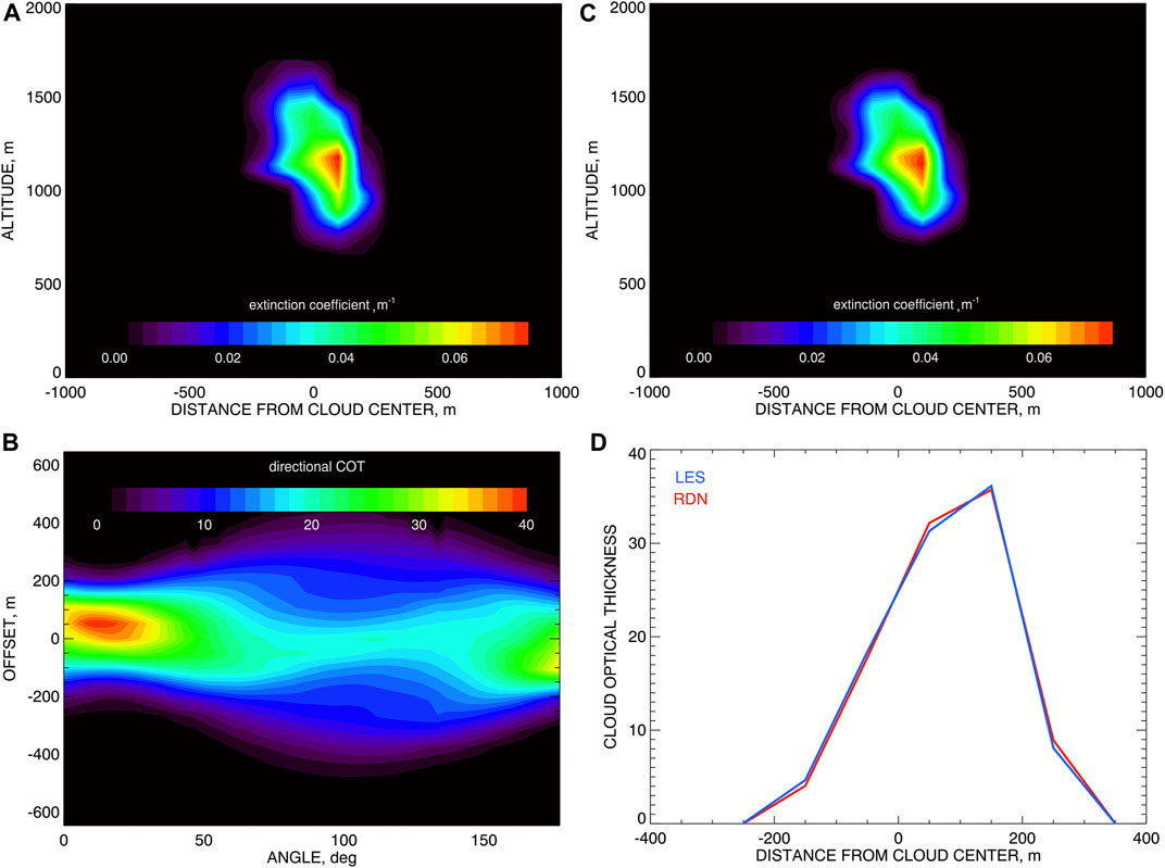
FIGURE 4. Test of Radon transform on a LES-generated cloud. (A) The initial 2D cross section of the cloud’s extinction coefficient distribution; (B) The directional COT tomogram derived from the field at (A) using direct Radon transform; (C) The result of inverse Radon transform applied to the tomogram at (B) (after calibration using the COT computed from the initial field); (D) The initial COT (blue) and that computed from the extinction field (from (C)) after calibration (red).

5 Derivation of Cloud Shapes From the Research Scanning Polarimeter Measurements

The RSP’s uniquely high angular resolution coupled with the high frequency of measurements can provide geometric constraints on the cumulus cloud’s 2D cross section and yield cloud’s geometric shape estimates (Alexandrov et al., 2016a). Use of a clear/cloud-separation threshold in the measured total reflectance allows for creation of a 1D cloud mask in each RSP scan distinguishing between the bright cloudy part of it and the darker background. The viewing angles at the edges of such cloud mask correspond to the view lines “tangent” to the cloud shape (given that the position of the aircraft relative to the cloud is accurately known). Figure 5 shows how the collection of all such tangent lines obtained during the overflight effectively “cuts out” a polygon (containing the cloud shape) in the 2D plane below the flight path (red and blue lines in Figure 5 correspond to different edges of 1D cloud masks). Then a disc-inscription technique is used to create a realistically-looking cloud shape within this polygon. In this method for each vortex of the polygon we create the largest disk with the center on the bisector of the corresponding corner, requiring that this disk is entirely contained inside the polygon’s interior (so it is tangent to some of the polygon’s edges). The boundary of the union of all such (usually overlapping) disks is then declared to be the shape of the cloud. In some cases (especially of elongated polygons) this technique does not work well, so the polygon itself provides a better representation of the cloud shape (Alexandrov et al., 2020).

FIGURE 5

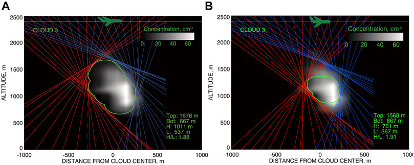
FIGURE 5. (A) derivation of the cloud shape (corresponding to the reflectance threshold of 0.0015) by cutting out a polygon in 2D space using the RSP view rays tangent to cloud surface and filling this polygon with a realistic cloud-shape curve. The initial droplet number concentration density is shown by grey-scale contour plot. This plot is reproduced from Alexandrov et al. (2016a). (B) Same as (A) but for the bright-cloud side threshold of 0.030 and the shadow-side threshold of 0.005.

A similar “space carving” methodology has been developed in a 3D case for the Multi-angle Imaging SpectroRadiometer (MISR) measurements (Lee et al., 2018). This technique is also used for the first-step definition of the cloud domain in the LSF tomographic algorithm described by Levis et al. (2020).

The notions of cloud shape or cloud boundary, while intuitively well-understood, are, strictly-speaking, quite ambiguous both in physical and optical sense. Physically, cloud is a spatially distributed collection of water droplets with no hard-defined surface. It can be artificially bounded by a level surface of the droplet number concentration corresponding to a threshold value chosen by the observer. Similarly, “optical surface” of the cloud can be defined using an arbitrarily chosen brightness threshold. It is affected by the solar and viewing geometries. For example, “optical surfaces” are systematically shifted relative “physical” ones towards the side of the cloud directly illuminated by the Sun. The higher is the brightness threshold, the smaller is the cloud-shape cutout derived using the technique described above.

However, while it is difficult to assign a precise physical meaning to the cloud shape corresponding to a single brightness threshold, the collection of such shapes derived for a range of thresholds may carry information about the internal structure of the cloud.

6 Reflectance-Proxy Density and Tomogram

In this study we assume that the reflectance measured by the RSP at a certain viewing angle is quantitatively one-to-one related to the directional COT (dCOT) along the corresponding view ray. This assumption allows us to use the measured reflectance to build dCOT tomogram, which will be then converted (using inverse Radon transform) into a 2D distribution of the cloud extinction coefficient. This assumption is, of course, a simplification in our essentially 3D setting, where multiple scattering within the whole cloud contributes to the reflectance at any particular direction. However, we will show below that this simplified assumption is sufficient for our purposes. When reflectance becomes a proxy for dCOT, it loses its optical properties and gains physical ones. Having this in mind, we introduce “reflectance-proxy” (RP) which coincides with the measured reflectance where it is present, while can be computed for other (virtual) view rays using inter- or extrapolation (in the same way as dCOT can be extended). Some of such view rays (e.g., horizontal ones) are inconsistent with the observation geometry and do not exist in real observation datasets. Also, the extended RP values are not expected to comply with the RT laws, so the RP is a rather abstract dataset that gets its physical meaning only after conversion to dCOT. This conversion will be discussed in Section 7.

Following the above assumptions we create an intermediate reflectance-proxy tomogram by interpolating the reflectances observed at the actual view rays to all possible view rays from a high-resolution grid of angles and offsets (relative to a chosen cloud center). This construction utilizes the collection of cloud shapes corresponding to a range of brightness thresholds. In a realistic analysis, the brightness threshold array consists of discrete values. The corresponding cloud shapes also form a discrete family, which is expected to be nested. Figure 6A presents such a cloud-shape family constructed for our simulated cloud using an array of 5 brightness thresholds. In addition to them, we may also use the maximum observed reflectance value that we associate with the cloud center depicted by white diamond in Figure 6A. Then, for each threshold we assign its value to all points of the corresponding cloud-shape curve. This operation converts the cloud shapes into level curves of an abstract 2D “reflectance-proxy distribution” (RPD), which then is extended to the entire 2D domain by interpolation between the RP values at the level-curve points. Specifically, for each point P in this domain we first select the two level curves (let us identify them as “1” and “2”) between which P is located. Then we determine the shortest distances from P to these two curves: d₁ and d₂ respectively. These distances are then used to compute the weights w₁ = d₂/(d₁ + d₂) and w₂ = d₁/(d₁ + d₂) with which the respective level-curves’ RP values contribute to the linearly interpolated value assigned to P. Moving-average smoothing takes care of interpolation irregularities. Our RPD is shown in Figure 6B. This RPD can be used for creation of cloud shapes corresponding to threshold values in-between of those from the initial discrete array, however, we use it in a different way.

FIGURE 6

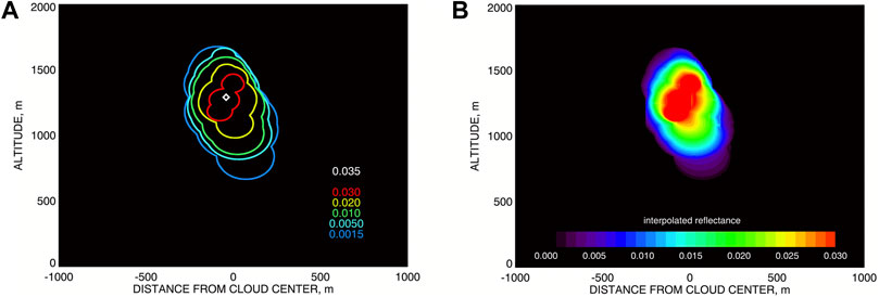
FIGURE 6. (A) The nested family of cloud shapes corresponding to five different reflectance thresholds; the maximal observed reflectance value is assigned to the point at the cloud’s center (depicted by white diamond). (B) The abstract reflectance distribution (RPD) computed by interpolation between the curves in the (A) assuming that each point of each curve is assigned the value equal to the corresponding brightness threshold.

Given the way the cloud shape corresponding to a certain brightness threshold is constructed, all the actual view rays tangent to it correspond to the same reflectance value equal to this of the threshold. We extend this property to all possible (not only actual) view rays tangent to this cloud shape. This, of course, is an abstraction not necessarily consistent with the nature of realistic light scattering within the cloud. This extension allows us to assign a RP value to any view ray (which from now on we will also call “chord”) crossing the RPD domain. The RP value assigned to a chord is this of the RPD’s level curve to which this chord is tangent. For the functional shape of the RPD in our case (which monotonically increases towards the cloud center) it is easy to see that this value is simply the maximum of the RPD along the chord.

In more complicated cases, such as e.g., two partially merged clouds, a chord may be tangent to two level curves with different values (each surrounding a different cloud center). In this case the along-chord RPD would have two local maxima, and the value of the larger of them should be assigned to the chord. This follows from the general structure of RPD with higher-value level curves being inside the interiors of the lower-value ones (since clouds are brighter at their center(s) than at their edges). So a chord coming from an observation with a lower threshold b cannot be tangent to a contour curve corresponding to a higher threshold a > b, since to do so it would have to cross another b-value level curve encompassing the a-value one (instead of being tangent to it). On the other hand, chords corresponding to a higher threshold a can cross level curves of any lower value since they are invisible for the a-based cloud masking.

While the RPD can be defined on a 2D grid with very fine resolution (we use 1 m, which certainly is an excess), the chords’ RP values can be also combined into a function of angles and offsets on a very fine grid (we use 1° resolution in angle and 1 m—in offset). This function is the RP tomogram R_tom (ψ, ρ). Figure 7A presents the RP tomogram computed for our cloud. Alongside determining the chords’ RPD maxima for the RP tomogram, we also collected the lengths of these chords when bounded by the cloud shape corresponding to the lowest brightness threshold (here 0.0015). These lengths also form a tomogram L_tom (ψ, ρ) defined on the same grid as R_tom (ψ, ρ); it is shown in Figure 7B.

FIGURE 7

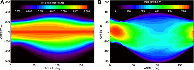
FIGURE 7. (A) The reflectance tomogram R_tom (ψ, ρ) computed for the RPD from Figure 6B by taking its maxima along the chords. (B) chord-length tomogram L_tom (ψ, ρ) consisting of the lengths of the same chords when bounded by the cloud shape corresponding to the lowest brightness threshold (0.0015).

7 From Reflectance-Proxy to Cloud Optical Thickness

On the next step of our analysis we need to find out how to relate the dCOT tomogram to the RP- and the chord-length-tomograms from Figure 7. Note that the dCOT tomogram can be determined up to an arbitrary constant factor, since the inverse Radon transform of it is also defined up to such a factor. The actual dCOT tomogram which we want to estimate from the RSP measurements is shown in Figure 4B. Note that using L_tom alone as the dCOT tomogram would result in a constant extinction value within the implied cloud domain. Indeed, having a constant extinction coefficient makes the dCOTs to be proportional to the corresponding chord lengths. This suggests that inclusion of L_tom into analysis together with R_tom would provide us with a better representation of the spatial configuration of the cloud.

Finding a good empirical proxy formula relating R_tom and L_tom to the dCOT tomogram τ_tom is a trial and error process, in which the LES data plays an active role (since we know what the result should be). After several trials we have stopped at the formula relating the reflectance R to the dCOT τ in the case of single scattering and normal incidence of a wide beam on a plane-parallel medium:

$R=\frac{1}{2}\left(1-e^{-2\tau }\right)b,(8)$

where b is a fitting parameter playing the role of the backscattering coefficient. It is assumed to be constant throughout the medium and not related to other physical parameters of the cloud; we use b = 0.1. Equation 8 translates into the following proxy formula for the dCOT tomogram

${\tau }_{\mathrm{t}\mathrm{o}\mathrm{m}}\left(\psi ,\rho \right)=-\ln \left[1-\frac{2}{b}{R}_{\mathrm{t}\mathrm{o}\mathrm{m}}\left(\psi ,\rho \right)\right]\frac{L_{\mathrm{t}\mathrm{o}\mathrm{m}}\left(\psi ,\rho \right)}{2\max L_{\mathrm{t}\mathrm{o}\mathrm{m}}}.(9)$

Here the denominator 2 max L_tom is actually irrelevant (since the inverse Radon transform of τ_tom is defined up to a constant factor) and is included only to make τ_tom dimensionless as dCOT should be. The dCOT tomogram for our cloud (with an arbitrary value scale) is presented in Figure 8A.

FIGURE 8

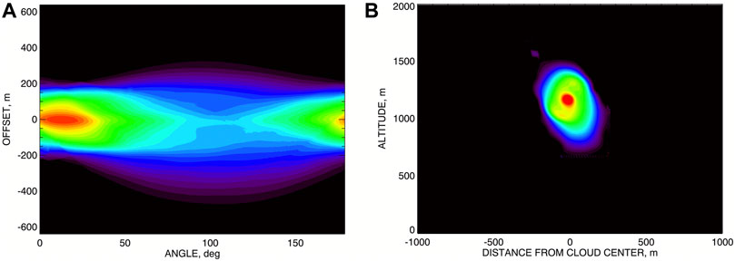
FIGURE 8. (A) The COT tomogram τ_tom (ψ, ρ) derived from R_tom and L_tom (Figure 7) using the proxy relation Eq. 9 (the units are irrelevant so no color bar is shown). (B) The spatial distribution of the extinction coefficient derived from τ_tom using inverse Radon transform and calibrated by the initial LES COT.

8 Calibration Issues

As we mentioned above, the extinction distribution derived from the dCOT tomogram using inverse Radon transform is defined up to an arbitrary constant factor and has to be calibrated. The calibration factor can be determined by iteratively computing the 3D-RT-simulated reflectances for scaled extinction fields until they match the RSP measurements. This way is computationally expensive and also involves uncertainties associated with the 2D nature of our retrievals that do not provide the full extent of the 3D cloud structure. A better alternative to this is to rely on additional measurements such as the COT derived from the RSP’s nadir reflectances using a LUT, or cloud-top extinction coefficient retrieved from the measurements made by the High Spectral Resolution Lidar (HSRL) which is often deployed on the same airborne platform as the RSP during field campaigns.

The algorithm for COT retrievals from the RSP’s nadir total reflectances uses a LUT computed assuming a plane-parallel geometry. Thus, while working fairly well for stratiform clouds, the retrievals for small popcorn Cu can be significantly affected by 3D effects such as leaking of scattered light through the cloud’s sides and shadowing (see e.g., Marshak et al., 1999; Várnai and Marshak, 2001; Várnai and Marshak, 2002). Both effects reduce the nadir reflectance (by about a factor of two in our case) compared to that from a stratiform cloud with the same COT. This causes significant underestimation of COT retrievals as long as the measurements are interpreted using plane-parallel LUT. Figure 9A illustrates this problem. Here the initial COT derived from the LES microphysics is shown in blue and has the maximum of about 35. The red curve represents the COT computed using the extinction field resulted from our tomographic procedure (Figure 8A) and rescaled to have the same maximum as the LES-derived COT. It is appeared to be shifted left by about 50 m towards the bright side of the cloud relative the blue curve. The solid green curve depicts the COT derived using the RSP’s nadir-view algorithm applied to the virtual RSP measurements. While being shifted to the left even further than the red curve, the value of the optically derived COT underestimates the microphysical one by the staggering factor of 4, and is certainly not suitable for calibration of the tomographic retrievals.

FIGURE 9

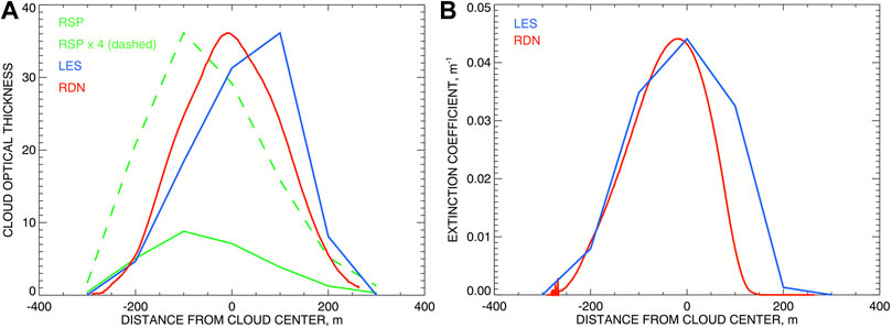
FIGURE 9. (A) Comparisons of COTs derived in different ways: by integration of the initial LES extinction field (blue), by integration of the backprojected field with subsequent scaling to match the LES COT maximum (red), and by applying the RSP algorithm to nadir-view reflectances (solid green; dashed green: the same multiplied by 4). (B) Horizontal profiles of the extinction coefficient at 1,400 m altitude: blue—from LES dataset, red—from tomographic retrievals scaled to match the maximum of the blue curve.

An alternative calibration method can be based on the extinction coefficient values at cloud top presumably known from HSRL retrievals. Figure 9B illustrates such scheme. Here we assume that virtual HSRL (which we do not currently simulate) provides accurate extinction coefficients (coinciding with the LES values) near cloud top (here at 1,400 m altitude). Then we find the calibration factor by scaling the tomographic extinction maximum at this altitude to match the maximum of the HSRL curve (shown in blue). The resulting tomographic extinction is shown in red. Application of this calibration factor to the tomographic COT results in only 16% overestimation (at maximum) of the LES COT from Figure 9A (and the same overestimation of the extinction coefficient).

We continue to explore the potential of the RSP’s own measurements of the polarized reflectance to provide the calibration constant. They are dominated by single scattering and, therefore, are less affected by 3D effects. However, for now, we want to separate calibration issues from assessing the accuracy of the characterization of the 2D cloud structure. For this purpose we adopt the calibration made by matching the tomographic COT maximum to the LES COT maximum. The tomographic COT then corresponds to the red COT-curve in Figure 9A. The extinction field in Figure 8B is calibrated accordingly. The same calibration is used in the comparisons presented below.

9 Comparison Between Research Scanning Polarimeter and LES Extinction Coefficients

Figure 10 presents the comparisons between the tomographic retrievals of the extinction coefficient from Figure 8B (right) with the initial LES extinction field. Plots in the left column of Figure 10 show that the retrieved field appears to be consistently shifted relative the original one by about 50 m to the left (towards the bright side of the cloud). This is a side effect of using brightness thresholds for derivation of cloud shapes: brighter parts of the cloud look optically and, therefore, physically thicker. Nevertheless, both fields show quite a structural similarity. To better demonstrate this in right-column plots we shifted the retrieved field to the right by 50 m, thus, improving the comparisons. Figure 10A shows color contour plot of the LES extinction coefficient (from Figure 4A) with the two level curves of the retrieved distribution being over-plotted. White curve corresponds to k_ext = 0.02 m⁻¹, black—to k_ext = 0.07 m⁻¹ (these values are represented by blue and red respectively in the color plot). We see quite good spatial agreement between the two fields in Figure 10A, left: within about 10 m both vertically and horizontally. The retrieved field also replicates the characteristic tilted-column shape of the initial cloud. For more detailed comparisons we plotted in Figure 10B the horizontal profiles of both fields along the transect at 1,100 m altitude. Similarly, Figure 10C compares vertical profiles of extinction coefficient along the transect at the cloud center.

FIGURE 10

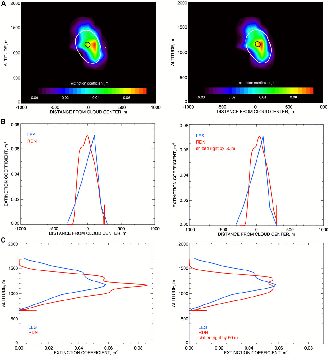
FIGURE 10. Comparison between the tomographic retrievals of the extinction coefficient from Figure 8B with the initial LES field. (A) Color contour plot of LES extinction coefficient with the level curves of the retrieved distribution being over-plotted: white curve corresponds to k_ext = 0.02 m⁻¹, black—to k_ext = 0.07 m⁻¹ (these values are represented by blue and red respectively in the color plot). (B) Same as top but along horizontal cross section at 1,100 m altitude. (C) same as top but along vertical cross section the cloud center. Left column presents the original retrievals, while in right column the retrieval field is shifted by 50 m to the right (away from the bright side of the cloud).

Figure 11 presents quantitative comparison between the retrieved extinction coefficient with that from the initial LES dataset. First, the retrieved k_ext field (with 1 m × 1 m spatial resolution) is interpolated to the LES data points (located on 100 m × 40 m grid). Then only the data points with positive values in both datasets are taken into comparison (to avoid the influence of zero-value points outside the cloud). The direct (as in Figure 10A, left) scatter-plot comparison of k_ext is presented in Figure 11A. Figure 11B shows the same type of comparison but with the retrieved field shifted to the right (away from the brighter cloud side) by 50 m (as in Figure 10B, right). The two datasets appear to be unbiased (having almost zero-mean difference) that is not surprising given that the LES COT was used to calibrate the RSP-derived extinction field. So the measure of the retrieval accuracy in this case is the standard deviation σ_k of the difference, which is 0.015 m⁻¹ (20.5% of the LES dataset’s maximum) for the un-shifted field and improves with the 50 m shift to 0.011 m⁻¹ (15.1% of the LES dataset’s maximum). The correlation between the two datasets also improves with the shift: from 73 to 84%. The LES extinction values used in this comparison have the mean of 0.023 m⁻¹, the median of 0.017 m⁻¹, and the maximum of 0.073 m⁻¹. The width of the scatter plot in Figure 11B does not seem to depend on the k_ext magnitude, so the best overall accuracy assessment is that 65% of the retrieval datapoints have extinction values within σ_k = ±0.01 m⁻¹ from their LES counterparts, and 96%—within 2σ_k = ±0.022 m⁻¹ (the corridor shown by dotted lines in Figure 11). For the un-shifted dataset 97% of points lie within its 2σ_k-corridor with the half-width of 0.030 m⁻¹.

FIGURE 11

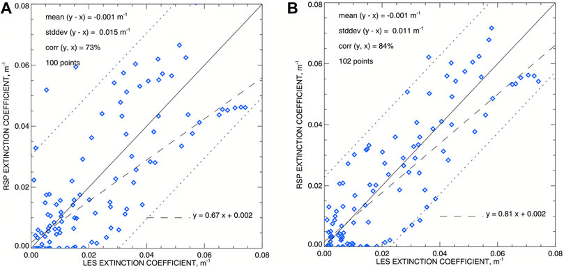
FIGURE 11. Quantitative comparison of the retrieved extinction coefficient with the initial data from the LES model. The retrieved k_ext field is interpolated to the LES data points. Only the data with above-zero values from both datasets are taken into comparison. (A) The original scatter plot of k_ext from both datasets. (B) Same as (A) but with the retrieved field shifted to the right (away from the brighter cloud side) by 50 m (as in Figure 10A, right). In each plot dashed line represents robust linear fit and two dotted lines bound 2σ_k-corridor around 1–1 solid line.

10 Derivation of Droplet Size Profiles Along the Cloud Side

Alexandrov et al. (2020) described a method for derivation of DSD vertical profiles from RSP-measured polarized reflectances. This method is a further development of our operational algorithms (Alexandrov et al., 2012a; Alexandrov et al., 2012b) based on the polarized rainbow analyses. The only new feature introduced by Alexandrov et al. (2020) was the aggregation of the RSP measurements to a range of points at the cloud’s side instead of the stereo-derived cloud top. The “cloud’s side” here is a part of the cloud-shape curve corresponding to some brightness threshold. Only points from the bright side of the cloud are considered. Note that in the case of a cloud tilted away from the Sun (as in Alexandrov et al., 2020) the stereo CTH on the bright side is usually close to a cloud-shape curve. Thus, the standard RSP DSD retrievals can be used for derivation of the profile without performing an alternative aggregation. This, however, is not the case for the cloud considered in this study which is slightly tilted toward the Sun.

The RSP-measured polarized reflectances are dominated by single scattering and are representative of the cloud layer of unit COT or about 50 m into the cloud (Alexandrov et al., 2018). Thus, the cloud shape chosen for derivation of a representative DSD profile should be somehow deeper into the cloud then the very first detectible curve corresponding to the smallest brightness threshold. On the other hand, the vertical extent of cloud shape rapidly decreases with the brightness threshold (as seen in Figure 6), thus, shortening the range of the corresponding DSD profile. In order to balance the range and representativeness of the profile we chose the cloud shape corresponding to two different thresholds one for the bright and the other for the shadowy sides of the cloud: 0.030 and 0.005 respectively (Figure 5B).

Figure 12A schematically illustrates aggregation of RSP measurements to a single point on the cloud surface from Figure 5B. The green lines represent the view rays (from different aircraft positions) corresponding to the view angles within the rainbow scattering range (135°–165°). Figure 12B shows the part of the cloud shape selected for derivation of the effective radius (Figure 12C) and variance (Figure 12D) profiles using the parametric fit method (Alexandrov et al., 2012a). Note that MYSTIC 3D RT code does not use bin-resolved DSDs (instead assuming gamma-distribution functional shapes with LES-derived r_eff and v_eff = 0.1). Hence, the non-parametric RFT retrieval technique (Alexandrov et al., 2012b) does not provide any additional information in this case.

FIGURE 12

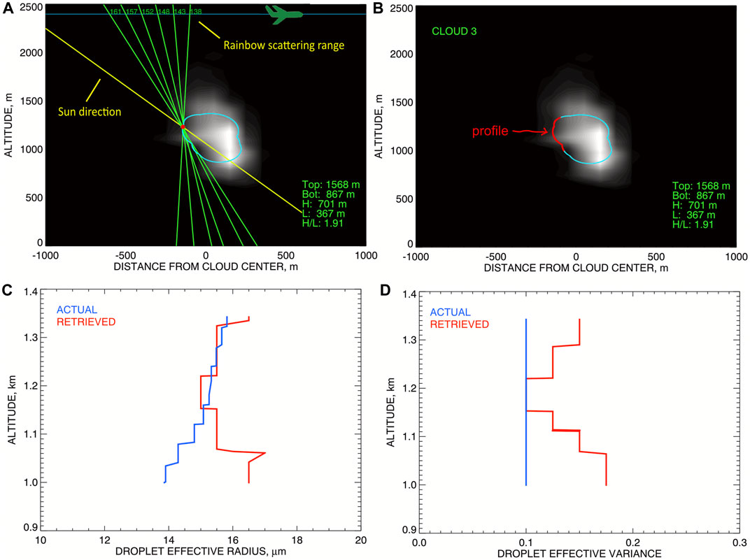
FIGURE 12. Derivation of droplet effective radius and variance profiles from RSP polarized reflectances aggregated to points along the cloud’s side. The cloud shape here is taken from Figure 5B. (A) Schematic representation of the method applied to a single point on the cloud surface. (B) The part of the cloud surface used for derivation of the profiles. (C) The droplet effective radius profiles (blue—from LES microphysics, red—retrieved from the RSP measurements). (D) Same as (C) but for the droplet effective variance.

Cloud-side profiles of DSD parameters appear to provide a good estimate of their inside-cloud counterparts both in simulated and real datasets. The 2D cross section of the r_eff distribution in our LES output presented in Figure 2B shows much stronger variation in the vertical dimension than in the horizontal one. Also, our statistical analysis of the data collected during CAMP²Ex demonstrated very good agreement (on average) between the DSD parameters derived from the RSP measurements at cloud tops and those measured in situ inside clouds when both datasets were plotted vs. their respective altitudes (these results will be published elsewhere). The LES model used by Levis et al. (2020) for demonstration of their LSF tomographic algorithm assumed the same r_eff profile and the same v_eff value of 0.1 throughout the cloud. While any LSF algorithm generally works as a “black box” not revealing dominant sources of specific retrievals, the tests performed by Martin and Hasekamp (2018) on simulated layer clouds suggest that the vertical profile information likely comes from the cloud side. They show that when the horizontal coverage of the cloud layer achieves 100% of the measurement domain (so its side is no longer seen) the retrievals loose any sensitivity to vertical profile.

In our case r_eff in Figure 12C and v_eff in Figure 12D both show little variability with altitude within the profile range. While the LES r_eff (blue curve) has a modest increase with height from 14 to 16 μm, this trend is not captured by the RSP retrievals (red curve). Thus, within our retrieval accuracy we can simply assume the constant values r_eff = 15.7 μm and v_eff = 0.14 throughout the cloud.

11 Droplet Number Concentration

The effective radius and variance profiles derived from the polarized reflectances at the cloud side are assumed to be good representations of the corresponding profiles inside the cloud (as we discussed in the previous section). Then the vertical profiles r_eff(h) and v_eff(h) can be used to obtain the 2D cross section of the droplet number concentration N_c(x, h) from that of the extinction coefficient k_ext (x, h) using Eq. 2:

$N_c\left(x,h\right)=\frac{k_{\mathrm{e}\mathrm{x}\mathrm{t}}\left(x,h\right)}{2\pi r_{\mathrm{e}\mathrm{ff}}^2\left(h\right)\left[1-v_{\mathrm{e}\mathrm{ff}}\left(h\right)\right]\left[1-2v_{\mathrm{e}\mathrm{ff}}\left(h\right)\right]}\times 10^6.(10)$

Here x and h are the horizontal and vertical coordinates respectively; N_c is measured in cm⁻³, k_ext—in m⁻¹.

In our case droplet size profiles are considered to be altitude-independent (r_eff = 15.7 μm, v_eff = 0.1), so N_c(x, h) is proportional to k_ext (x, h) and its plot in Figure 13A is a rescaled version of that in Figure 8B. Figure 13B presents comparison of the retrieved N_c with the initial LES field (shown in color). Over-plotted white curve is the level curve of the retrieved N_c (Figure 13A) corresponding to 20 cm⁻³, black curve corresponds to the 60 cm⁻³ level (these level values are represented by blue and red respectively in the color plot). As in Figure 10A (right) the retrieval curves here are shifted to the right by 50 m. Comparisons between retrieved (red) and initial LES (blue) droplet number concentrations for the horizontal transect at 1,100 m altitude and the vertical transect at the cloud center are presented in Figures 13C,D, respectively. Retrieved N_c field in both bottom plots is also shifted by 50 m to the right.

FIGURE 13

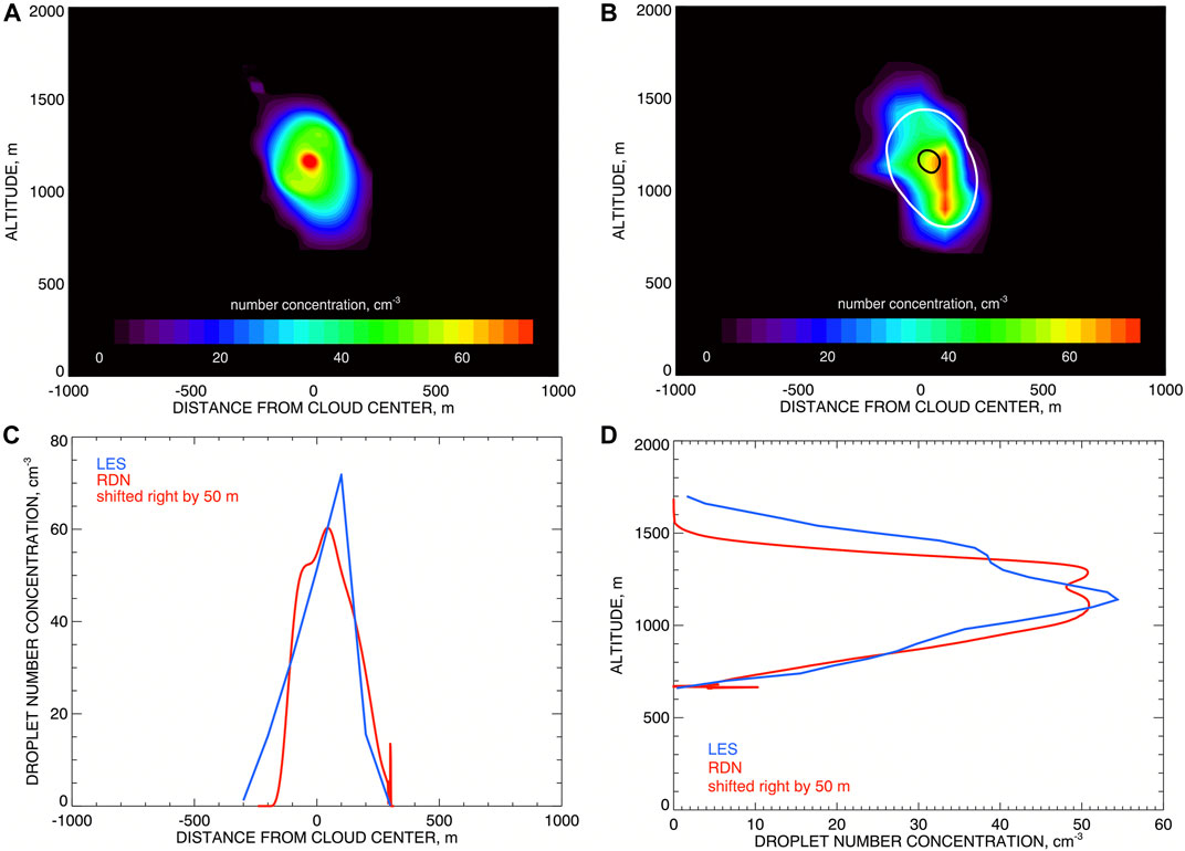
FIGURE 13. (A) spatial distribution of droplet number concentration derived from the extinction coefficient in Figure 8B using Eq. 10 with r_eff = 15.5 μm and v_eff = 0.1 (from Figures 12C,D). (B) Comparison of the retrieved N_c with the initial LES field (shown in color); over-plotted white curve corresponds to retrieved N_c = 20 cm⁻³, black—to N_c = 60 cm⁻³ (these values are represented by blue and red respectively in the color plot); both retrieved curves are shifted to the right by 50 m. (C) Comparison between retrieved (red) and initial LES (blue) droplet number concentrations for the horizontal transect at 1,100 m altitude. (D) Same as (C) but for the vertical transect at the cloud center. The retrieved N_c fields in both bottom plots are shifted by 50 m to the right.

Figure 14 presents quantitative comparison of the retrieved N_c values with those in the LES dataset. As in Figure 11 the retrievals are interpolated to the LES data points. Only the points with N_c > 1 cm⁻³ and positive k_ext (i.e., positive r_eff) in both datasets were selected for the comparison. The LES N_c values have the mean of 28.75 cm⁻³, median of 28.36 cm⁻³, and maximum of 71.74 cm⁻³. Figure 14A shows the original scatter plot, while in the right panel the retrieved field is shifted to the right by 50 m (as in Figure 13B). The droplet number concentration comparisons are not as good as those of the extinction coefficient due to limited accuracy of our retrieved droplet size profiles. However, they demonstrate the possibility of quantitative estimation of 2D N_c field. There are very small negative biases in both plots (less than 0.5 cm⁻³), while the standard deviation σ_n provides more definitive accuracy estimate. As expected, the accuracy improves with the shift from 17.6 to 12.8 cm⁻³, while the correlation increases from 65 to 81%. In Figure 14A 96.5% of points lie within the 2σ_n-corridor (depicted by two dotted lines). The shift does not change this number much (97.7%) while the corridor is visibly narrower in Figure 14B. Thus, we can estimate our accuracy of N_c retrievals as ±13 cm⁻³, regardless of the N_c value (within the range of our model), which in this case constitutes 17% of the maximal N_c and 43% of its mean or median.

FIGURE 14

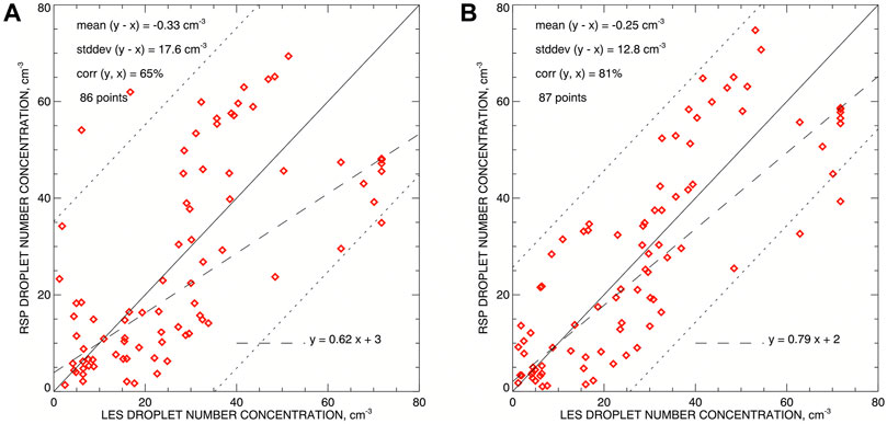
FIGURE 14. Quantitative comparison between the retrieved droplet number concentration and the initial one from the LES model. The retrieved N_c field is interpolated to the LES data points. Only the data points with N_c > 1 cm⁻³ in both datasets are taken into comparison. (A) The original scatter plot of N_c from both datasets. (B) Same as (A) but with the retrieved field shifted to the right (away from the brighter cloud side) by 50 m (as in Figure 13B).

The ability to derive 2D droplet number concentration field opens possibility to calibrate tomographic retrievals using in situ measurements inside the cloud.

12 Conclusion

We presented a new remote sensing tomographic technique allowing for retrieval of cloud internal structure from external measurements made by the Research Scanning Polarimeter. While tomography (in narrow sense) is an active technique incompatible with the geometry of atmospheric remote sensing, we developed a “semi-tomographic” approach in which the tomogram of the cloud is estimated from passive measurements instead of being measured directly. This tomogram is then converted into spatial distribution of extinction coefficient using inverse Radon transform (filtered backprojection), which is the standard procedure in the actual tomography (used e.g., in medical CT scans). This procedure is computationally inexpensive compared to approaches relying on multi-dimensional least-square fitting since it does not require iterative 3D RT simulations.

We illustrated and validated the proposed technique using simulated RSP observations of a LES-generated Cu cloud. The radiation field was computed using MYSTIC 3D RT code. On the first step of our algorithm we use the RSP’s view rays grazing the cloud “surface” to create a nested family of cloud shapes corresponding to a range of radiometric thresholds. This family is used for estimation of the “reflectance tomogram” which is then converted into COT tomogram using the proxy relation Eq. 9. While this empirical relation is the result of an educated guess, its validity has been proven using the simulated data.

In the second step Radon transform is applied to the COT tomogram resulting in 2D distribution of the extinction coefficient defined up to an unknown constant factor. To determine this factor a calibration procedure based on additional data should be used. While the RSP’s own measurements would be preferable for the calibration, this appeared to be problematic. Our first choice of the calibration dataset was the RSP-derived nadir COT (given that the LES-derived COT was successfully used for self-test of Radon transform on the LES data). However, unfortunately, the COT derived from the RSP’s nadir measurements assuming plane-parallel geometry appeared to have a significant low bias due to 3D effects (e.g., leaking of light through the cloud’s sides) and could not be used for calibration. We consider the RSP’s polarized reflectance as a potential calibration source since it is dominated by single scattering and is less sensitive to 3D effects. Alternatively, the values of extinction coefficient at cloud top derived from correlative lidar measurements can be also used (this is a relatively new data product developed by the HSRL team). In our simulations we found that this type of calibration leads to a rather modest 16% overestimation of the overall 2D extinction values and the COT. While more work is needed to resolve the calibration issues, in this study we wanted to estimate the accuracy of the method apart from the calibration uncertainty. To do this we used the “ideal” calibration based on the LES-derived COT (assuming that it is known from a hypothetical independent measurement).

The reflectance-based cloud shapes at the first step of our algorithm are naturally shifted towards the bright side of the actual cloud and this bias propagates to the retrieved 2D extinction field. Thus, a point-by-point comparison of this field with the initial LES-derived distribution showed notable improvements after 50 m shifting away from the bright side of the cloud. We understand that at different cloud and illumination conditions the optimal shift may be also different. However, in real remote sensing the retrievals of cloud’s physical structure are more important than that of its exact location, so an error in the latter can be tolerated (see Supplementary Material for other potential sources of the retrieval uncertainties). The retrievals of the extinction coefficient appeared to be unbiased in value, so we measured the retrieval uncertainty using the standard deviation σ_k of the difference with the LES values. We found that for the shifted dataset σ_k = 0.01 m⁻¹ (13.7% of the LES dataset’s maximum) and 98% of the retrieved values of k_ext lie within 2σ_k = 0.02 m⁻¹ from their LES counterparts.

In the next step we converted the extinction retrievals into these of cloud droplet number concentration N_c. In order to do this we first estimated the droplet size distribution parameters (effective radius and variance) within the cloud. We assume (based by the LES data) that the DSD-parameters profiles do not significantly vary in the horizontal direction (which may not be the case for other real or simulated clouds). This allows us to use throughout the cloud the profiles of r_eff and v_eff derived from the RSP’s polarized reflectance measurements made along the cloud side. These retrievals were made using the rainbow (cloud bow) fitting technique (Alexandrov et al., 2012a; Alexandrov et al., 2018). In our example both DSD parameters appeared to be nearly constant within the retrieval accuracy and vertical range making the conversion of the 2D k_ext field into the spatial distribution of N_c particularly straightforward (just a rescaling). As in the extinction case the comparison of the N_c retrievals with the corresponding LES values improves with the 50 m shift achieving the accuracy (the standard deviation of the difference) σ_n = 12.3 cm⁻³ (17% of the maximal N_c) while 95.3% of the points in the scatter plot lie within the 2σ_n-corridor. The correlation between the two datasets is 80%.

In the upcoming continuation of this series we will present examples of tomographic analyzes of real clouds observed during NASA’s Cloud, Aerosol and Monsoon Processes Philippines Experiment (CAMP²Ex) conducted in 2019. During this campaign the RSP was deployed on-board of NASA’s P3-B aircraft together with a number of other remote-sensing and in situ instruments, measurements of which we can use to both improve and validate our retrievals. In particular, we plan to use the extinction coefficients at cloud top derived from the measurements made by the High Spectral Resolution Lidar (HSRL2) to calibrate our tomographic extinction field, while the HSRL cloud-top height product will be used to validate our retrievals of the cloud geometry. We will also look at the measurements from the Airborne Precipitation Radar (APR-3) to validate our retrievals of cloud shape and position.

A detailed analysis of the requirements to the sensor’s angular range and resolution will be also presented in our future publications (with different RSP platforms in mind, as well as other airborne and satellite instruments). Some preliminary estimates of the tomographic retrieval accuracy are presented in Supplementary Material accompanying this paper.

Data Availability Statement

The raw data supporting the conclusion of this article will be made available by the authors, without undue reservation.

Author Contributions

MA conceived, designed and applied the tomographic algorithm to sample synthetic and real data. CE performed 3D RT computations using LES dataset created by A. Ackerman. BC and BD provided expertise on Radiative Transfer, the RSP’s measurements and operations as well as on other available field-campaign datasets. They also advised on the requirements to the RSP-based algorithms for their implementation into the upcoming NASA PACE satellite mission.

Funding

This research was funded by the NASA Radiation Sciences Program managed by Hal Maring and NASA grants NNH16ZDA001N-CAMP2EX and NNH19ZDA001N-PACESAT.

Conflict of Interest

The authors declare that the research was conducted in the absence of any commercial or financial relationships that could be construed as a potential conflict of interest.

Publisher’s Note

All claims expressed in this article are solely those of the authors and do not necessarily represent those of their affiliated organizations, or those of the publisher, the editors, and the reviewers. Any product that may be evaluated in this article or claim that may be made by its manufacturer is not guaranteed or endorsed by the publisher.

Acknowledgments

We would like to thank A. S. Ackerman for generating the LES datasets that we keep using in our studies for many years, including this publication. We also want to thank L. Di Girolamo for encouragement of this work and for useful discussions.

Supplementary Material

The Supplementary Material for this article can be found online at: https://www.frontiersin.org/articles/10.3389/frsen.2021.791130/full#supplementary-material

References

Ackerman, A. S., Kirkpatrick, M. P., Stevens, D. E., and Toon, O. B. (2004). The Impact of Humidity above Stratiform Clouds on Indirect Aerosol Climate Forcing. Nature 432, 1014–1017. doi:10.1038/nature03174

PubMed Abstract | CrossRef Full Text | Google Scholar

Alexandrov, M. D., Ackerman, A. S., and Marshak, A. (2010). Cellular Statistical Models of Broken Cloud fields. Part II: Comparison with a Dynamical Model and Statistics of Diverse Ensembles. J. Atmos. Sci. 67, 2152–2170. doi:10.1175/2010jas3365.1

CrossRef Full Text | Google Scholar

Alexandrov, M. D., Cairns, B., Emde, C., Ackerman, A. S., Ottaviani, M., and Wasilewski, A. P. (2016a). Derivation of Cumulus Cloud Dimensions and Shape from the Airborne Measurements by the Research Scanning Polarimeter. Remote Sensing Environ. 177, 144–152. doi:10.1016/j.rse.2016.02.032

CrossRef Full Text | Google Scholar

Alexandrov, M. D., Cairns, B., Emde, C., Ackerman, A. S., and van Diedenhoven, B. (2012a). Accuracy Assessments of Cloud Droplet Size Retrievals from Polarized Reflectance Measurements by the Research Scanning Polarimeter. Remote Sensing Environ. 125, 92–111. doi:10.1016/j.rse.2012.07.012

CrossRef Full Text | Google Scholar

Alexandrov, M. D., Cairns, B., and Mishchenko, M. I. (2012b). Rainbow Fourier Transform. J. Quantitative Spectrosc. Radiative Transfer 113, 2521–2535. doi:10.1016/j.jqsrt.2012.03.025

CrossRef Full Text | Google Scholar

Alexandrov, M. D., Cairns, B., Sinclair, K., Wasilewski, A. P., Ziemba, L., Crosbie, E., et al. (2018). Retrievals of Cloud Droplet Size from the Research Scanning Polarimeter Data: Validation Using In Situ Measurements. Remote Sensing Environ. 210, 76–95. doi:10.1016/j.rse.2018.03.005

CrossRef Full Text | Google Scholar

Alexandrov, M. D., Cairns, B., van Diedenhoven, B., Ackerman, A. S., Wasilewski, A. P., McGill, M. J., et al. (2016b). Polarized View of Supercooled Liquid Water Clouds. Remote Sensing Environ. 181, 96–110. doi:10.1016/j.rse.2016.04.002

CrossRef Full Text | Google Scholar

Alexandrov, M. D., Cairns, B., Wasilewski, A. P., Ackerman, A. S., McGill, M. J., Yorks, J. E., et al. (2015). Liquid Water Cloud Properties during the Polarimeter Definition Experiment (PODEX). Remote Sensing Environ. 169, 20–36. doi:10.1016/j.rse.2015.07.029

CrossRef Full Text | Google Scholar

Alexandrov, M. D., Miller, D. J., Rajapakshe, C., Fridlind, A., van Diedenhoven, B., Cairns, B., et al. (2020). Vertical Profiles of Droplet Size Distributions Derived from Cloud-Side Observations by the Research Scanning Polarimeter: Tests on Simulated Data. Atmos. Res. 239, 104924. doi:10.1016/j.atmosres.2020.104924

PubMed Abstract | CrossRef Full Text | Google Scholar

Cairns, B., Russell, E. E., and Travis, L. D. (1999). “Research Scanning Polarimeter: Calibration and Ground-Based Measurements,” in Polarization: Measurement, Analysis, and Remote Sensing. Editors DH Goldstein, and DB Chenault (Denver, Colorado: Proc. SPIE), 3754, 186–197.

Google Scholar

Emde, C., Buras, R., Mayer, B., and Blumthaler, M. (2010). The Impact of Aerosols on Polarized Sky Radiance: Model Development, Validation, and Applications. Atmos. Chem. Phys. 10, 383–396. doi:10.5194/acp-10-383-2010

CrossRef Full Text | Google Scholar

Hansen, J. E., and Travis, L. D. (1974). Light Scattering in Planetary Atmospheres. Space Sci. Rev. 16, 527–610. doi:10.1007/bf00168069

CrossRef Full Text | Google Scholar

Lee, B., Di Girolamo, L., Zhao, G., and Zhan, Y. (2018). Three-Dimensional Cloud Volume Reconstruction from the Multi-Angle Imaging SpectroRadiometer. Remote Sensing 10, 1858. doi:10.3390/rs10111858

CrossRef Full Text | Google Scholar

Levis, A., Schechner, Y. Y., Davis, A. B., and Loveridge, J. (2020). Multi-View Polarimetric Scattering Cloud Tomography and Retrieval of Droplet Size. Remote Sensing 12, 2831. doi:10.3390/rs12172831

CrossRef Full Text | Google Scholar

Marshak, A., Oreopoulos, L., Davis, A. B., Wiscombe, W. J., and Cahalan, R. F. (1999). Horizontal Radiative Fluxes in Clouds and Accuracy of the Independent Pixel Approximation at Absorbing Wavelengths. Geophys. Res. Lett. 26, 1585–1588. doi:10.1029/1999gl900306

CrossRef Full Text | Google Scholar

Martin, W. G. K., and Hasekamp, O. P. (2018). A Demonstration of Adjoint Methods for Multi-Dimensional Remote Sensing of the Atmosphere and Surface. J. Quantitative Spectrosc. Radiative Transfer 204, 215–231. doi:10.1016/j.jqsrt.2017.09.031

CrossRef Full Text | Google Scholar

Mayer, B. (2009). Radiative Transfer in the Cloudy Atmosphere. Eur. Phys. J. Conferences 1, 75–99. doi:10.1140/epjconf/e2009-00912-1

CrossRef Full Text | Google Scholar

Mishchenko, M. I., Cairns, B., Kopp, G., Schueler, C. F., Fafaul, B. A., Hansen, J. E., et al. (2007). Accurate Monitoring of Terrestrial Aerosols and Total Solar Irradiance: Introducing the Glory mission. Bull. Amer. Meteorol. Soc. 88, 677–692. doi:10.1175/bams-88-5-677

CrossRef Full Text | Google Scholar

M. I. Mishchenko, CL Parkinson, A Ward, and MD King (Editors) (2006). Glory, in Earth Science Reference Handbook: A Guide to NASA’s Earth Science Program and Earth Observing Satellite Missions (Washington, DC: National Aeronautics and Space Administration), 141–147.

Google Scholar

Nakajima, T., and King, M. D. (1990). Determination of the Optical Thickness and Effective Particle Radius of Clouds from Reflected Solar Radiation Measurements. Part I: Theory. J. Atmos. Sci. 47, 1878–1893. doi:10.1175/1520-0469(1990)047<1878:dotota>2.0.co;2

CrossRef Full Text | Google Scholar

Radon, J. (1917). “Über die Bestimmung von Funktionen durch ihre Integralwerte längs gewisser Mannigfaltigkeiten,” in Berichte über die Verhandlungen der Königlich-Sächsischen Akademie der Wissenschaften zu Leipzig (Leipzig: Mathematisch-Physische Klasse Teubner), 69, 262–277.

Google Scholar

Radon, J., and Parks, P. C. (translator) (1986). On the Determination of Functions from Their Integral Values along Certain Manifolds. IEEE Trans. Med. Imaging 5, 170–176. doi:10.1109/tmi.1986.4307775

PubMed Abstract | CrossRef Full Text | Google Scholar

Sinclair, K., van Diedenhoven, B., Cairns, B., Alexandrov, M., Moore, R., Crosbie, E., et al. (2019). Polarimetric Retrievals of Cloud Droplet Number Concentrations. Remote Sens. Environ. 228, 227–240. doi:10.1016/j.rse.2019.04.008

CrossRef Full Text | Google Scholar

Sinclair, K., van Diedenhoven, B., Cairns, B., Yorks, J., Wasilewski, A., and McGill, M. (2017). Remote Sensing of Multiple Cloud Layer Heights Using Multi-Angular Measurements. Atmos. Meas. Tech. 10, 2361–2375. doi:10.5194/amt-10-2361-2017

CrossRef Full Text | Google Scholar

van Zanten, M. C., Stevens, B. B., Nuijens, L., Siebesma, A. P., Ackerman, A., Burnet, F., et al. (2011). Controls on Precipitation and Cloudiness in Simulations of Trade-Wind Cumulus as Observed during RICO. J. Adv. Model. Earth Syst. 3, M06001. doi:10.1029/2011ms000056

CrossRef Full Text | Google Scholar

Várnai, T., and Marshak, A. (2002). Observations and Analysis of Three-Dimensional Radiative Effects that Influence MODIS Cloud Optical Thickness Retrievals. J. Atmos. Sci. 59, 1607–1618. doi:10.1175/1520-0469(2002)059<1607:OOTDRE>2.0.CO;2

CrossRef Full Text | Google Scholar

Várnai, T., and Marshak, A. (2001). Statistical Analysis of the Uncertainties in Cloud Optical Depth Retrievals Caused by Three-Dimensional Radiative Effects. J. Atmos. Sci. 58, 1540–1548. doi:10.1175/1520-0469(2001)058<1540:SAOTUI>2.0.CO;2

CrossRef Full Text | Google Scholar

Werdell, P. J., Behrenfeld, M. J., Bontempi, P. S., Boss, E., Cairns, B., Davis, G. T., et al. (2019). The Plankton, Aerosol, Cloud, Ocean Ecosystem Mission: Status, Science, Advances. Bull. Amer. Meteorol. Soc. 100, 1775–1794. doi:10.1175/bams-d-18-0056.1

CrossRef Full Text | Google Scholar