 Frederiek C. Sperna Weiland1*
 Robrecht D. Visser1,2,3
 Peter Greve4
 Berny Bisselink5
 Lukas Brunner6
 Albrecht H. Weerts1,3
- 1Inland Water Systems, Deltares, Delft, Netherlands
- 2Witteveen+Bos Consulting Engineers, Deventer, Netherlands
- 3Hydrology and Quantitative Water Management Group, Department of Environmental Sciences, Wageningen University and Research, Wageningen, Netherlands
- 4Water Security Research Group, Biodiversity and Natural Resources Program, International Institute for Applied Systems Analysis, Laxenburg, Austria
- 5European Commission, Joint Research Centre, Ispra, Italy
- 6Institute for Atmospheric and Climate Science, ETH Zurich, Zurich, Switzerland
Ensemble projections of future changes in discharge over Europe show large variation. Several methods for performance-based weighting exist that have the potential to increase the robustness of the change signal. Here we use future projections of an ensemble of three hydrological models forced with climate datasets from the Coordinated Downscaling Experiment - European Domain (EURO-CORDEX). The experiment is set-up for nine river basins spread over Europe that hold different climate and catchment characteristics. We evaluate the ensemble consistency and apply two weighting approaches; the Climate model Weighting by Independence and Performance (ClimWIP) that focuses on meteorological variables and the Reliability Ensemble Averaging (REA) in our study applied to discharge statistics per basin. For basins with a strong climate signal, in Southern and Northern Europe, the consistency in the set of projections is large. For rivers in Central Europe the differences between models become more pronounced. Both weighting approaches assign high weights to single General Circulation Models (GCMs). The ClimWIP method results in ensemble mean weighted changes that differ only slightly from the non-weighted mean. The REA method influences the weighted mean more, but the weights highly vary from basin to basin. We see that high weights obtained through past good performance can provide deviating projections for the future. It is not apparent that the GCM signal dominates the overall change signal, i.e., there is no strong intra GCM consistency. However, both weighting methods favored projections from the same GCM.
Introduction
Throughout Europe the hydrological cycle is changing as a result of anthropogenic induced global warming (Kreibich et al., 2014; Alfieri et al., 2015; Gudmundsson et al., 2017). Changes in extreme weather are expected to significantly influence flood risk and water availability (Kundzewicz et al., 2017). Numerous impact assessments have been conducted at European and river basin scale (Alfieri et al., 2015; Forzieri et al., 2016; Thober et al., 2018; Blöschl et al., 2019). For individual rivers, changes in flood hazard provided by different studies have not always been in agreement (Kundzewicz et al., 2017). In general, the simulated direction and magnitude of changes in the hydrological cycle depends on the geographic positioning, catchment characteristics and river networks (Acreman and Sinclair, 1986; Beven et al., 1988) as well as the local anticipated meteorological changes. The larger the natural climate variability, the harder it will be for the models to capture the natural hydrological processes. Past studies showed that climate impacts are expected to differ for Southern and Northern Europe (Dankers and Feyen, 2008; Stahl et al., 2010; Gudmundsson et al., 2017; Blöschl et al., 2019). This will very likely lead to increased seasonal water constraints in Southern Europe and abundant water availability in the North (e.g., Greve et al., 2018). However, a large area in Europe is in a transition zone between a wetter northern and a drier southern future climate where climate models often disagree on the sign of change (Giorgi and Coppola, 2007).
For climate impact assessments at the river basin scale, ideally Regional Climate Models (RCMs) are used. To this end the EURO-CORDEX initiative developed an ensemble of RCM simulations at a horizontal resolution of ~11 km (0.11°). These high-resolution RCMs can provide more regional details on future change and give a better representation of daily high intensity rainfall (Jacob et al., 2014) than General Circulation Models (GCMs). Apart from the hydrological model, its parametrization and the uncertainties in the RCM, the forcing GCM creates an additional uncertainty to the modeling effort for complex natural systems (Melsen et al., 2018). To minimalize this uncertainty, the availability of a large ensemble of RCMs forced by different GCMs allows for an improved estimation of the spread and inherent uncertainties of future climate projections (Clark et al., 2016). Yet, within the ensemble the driving GCMs are not necessarily independent from each other and might share several components affecting the proximity of their results (Boé, 2018). Pennell and Reichler (2011) indicated that this can lead to overconfident climate projections. Moreover, not all GCMs are equally skillful in projecting the climate of a certain region or the historical temperature response to greenhouse gas emissions (e.g., Eyring et al., 2019).
Different methods such as weighting models from GCM ensembles by their performance and independence have been developed to account for these factors, to reduce the uncertainty introduced by the GCMs, and to provide more confident projections of future climate (e.g., Knutti et al., 2017; Brunner et al., 2020). Recently, Brunner et al. (2019) applied the Climate model Weighting by Independence and Performance (ClimWIP) method to temperature and precipitation projections in several European sub-regions. ClimWIP is based on earlier work by Sanderson et al. (2015a,b), Knutti et al. (2017), and Lorenz et al. (2018). The method is freely available as part of ESMValTool (docs.esmvaltool.org). Focusing on regional meteorological indices, these studies showed that GCM weighting reduces the spread between projections and can increase the skill of projected changes.
An alternative for weighting is sub-selecting climate models from the full ensemble set based on characteristics like similarity and performance. Sub-selecting aims at the reduction of computational costs running the full modeling chain only for a smaller informative set of climate models (Kiesel et al., 2019). Kiesel et al. (2020) compared a variety of weighting and selection methods that amongst others consider (1) model performance for the historic period, (2) the representation of ensemble model diversity which could help to level out representation errors in singe models and (3) representation of trends which are an indication of the direction and rate of change. They already stated that changes in precipitation and temperature impact streamflow through complex non-linear hydrological processes such as soil infiltration, evapotranspiration and runoff generation. Therefore, in this study, next to the weighting method of Brunner et al. (2019), we also derive weighted hydrological responses based on hydrological model performance and similarity in projected change for specific discharge characteristics (Giorgi and Mearns, 2002; Sperna Weiland et al., 2012).
To consistently assess the variation in discharge change patterns we focus on 9 river basins spread over Europe that are together considered to represent European catchment characteristics and climate conditions well. To allow for a spatially uniform assessment and to estimate the uncertainty introduced by the hydrological model. We have used the same three hydrological models for each of the basin considered. It was decided to base this study on available simulations. The different hydrological model experiment setups are not fully consistent, but all represent contemporary approaches to project hydrological change from climate change signals.
The three models are the calibrated hydrological models LISFLOOD (Van Der Knijff et al., 2010) and CWatM (Burek et al., 2020) which can both simulate at a variable grid-scale resolution dependent on the area of interest. With this variable resolution the models can provide an improved representation of small scale processes that cannot be captured with the original coarse model grids. The third model is the distributed hydrological model wflow_sbm which parameterization is based on global datasets of physical catchment characteristics. The model is implemented at basin scale and (sub-)kilometer resolution (Imhoff et al., 2020; Eilander et al., 2021). Only for the simulations with LISFLOOD a bias-correction of the CORDEX data was applied. As mentioned before several studies already exist that focus on future hydrological changes on a continental or global scale based on a set of hydrological and climate models (Haddeland et al., 2011; Pokhrel et al., 2021). The additional step taken in this study is the weighting approach which is, due to its ability to reduce uncertainties, extremely relevant for water management and plan making based upon these projections.
Data and Methods
Catchments
This study explores the impact of the projected climate change on river discharge characteristics of nine catchments spread over Europe. These nine catchments were chosen based on their size, climate conditions and geographical position (Figure 1). The catchment characteristics are shown in Table 1.
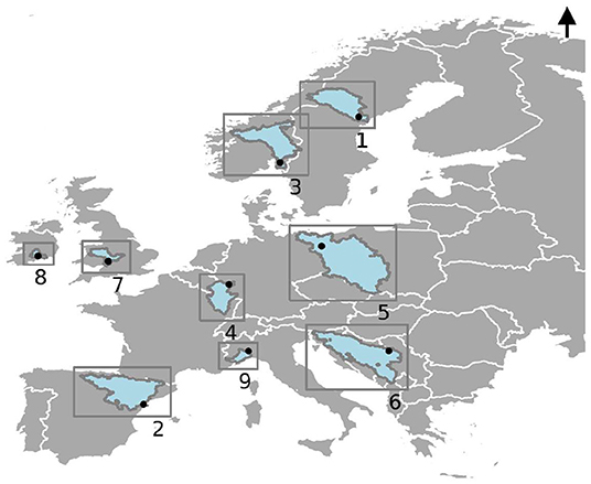
Figure 1. Geographical position of the catchments in Europe. Numbers indicate the river basins; the Ångermanälven (1), Ebro (2), Glomma (3), Moselle (4), Oder (5), Sava (6), Severn (7), Suir (8), and Tanaro (9). Dots indicate the gauge locations used in this study.
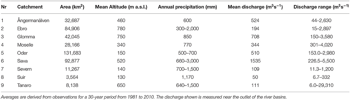
Table 1. Characteristics of studied catchments.
Models
wflow_sbm
The distributed hydrological model wflow_sbm is a conceptual bucket model with a kinematic wave routing approach for lateral subsurface, overland and river flow processes that is similar to TOPKAPI (Todini and Ciarapica, 2002). The model has a simplified physical basis with parameters that represent physical characteristics, leading to a relatively easy linkage of the parameter values to actual physical properties (Imhoff et al., 2020). The model parameters are estimated a priori using transfer functions (Imhoff et al., 2020) and available global or local datasets. Using these transfer functions and upscaling rules, wflow_sbm can be set up at various model resolutions (here 0.00833 degree, ~1 km) for any catchment. The model has a spatially distributed gridded cell network with the presence of lateral subsurface flow based on a D8-network flow routing network. The soil is divided in saturated and unsaturated store(s) and can be divided in any number of layers (here 3). Vertical transfer of water is controlled by saturated hydraulic conductivity, the effective saturation degree of the layer and the Brooks-Corey power coefficient (based on pore size distribution). Lateral subsurface flow, overland and river flow between grid cells is routed using the kinematic equation. Water can be lost through evapotranspiration and interception based on the Gash (1979) or Rutter et al. (1971) model depending on the timestep (here day). wflow_sbm has a sub-module to simulate glacier buildup and melting processes. The model includes lakes and reservoirs, simple reservoir regulation (e.g., H-Q tables) can be included. A priori values for reservoir demand, targets for full and minimum reservoir fractions are derived from available dataets. For more information, we refer to Imhoff et al. (2020), Eilander et al. (2021). The wflow_sbm source code is available under the MIT license from github (https://github.com/Deltares). The hydromt code to setup the models including a priori parameters is also available under the MIT license from github (https://github.com/Deltares). The model requires daily estimates of precipitation, temperature, radiation, and surface air pressure as inputs to calculate potential evaporation using the De Bruin method (De Bruin, 1983).
Wflow_sbm parameter estimation is based on available spatial datasets providing information on soil properties, soil depth, rooting depth etc. Imhoff et al. (2020) developed a method to parameterize the model for any basin in the world using regionalization methods based on literature (pedo)transfer functions and upscaling techniques. Only for the Horizontal Hydraulic Conductivity Fraction (KsatHorFrac) there is no pedo-transfer function, this is a rather sensitive parameter in the model. In order to calibrate the KsatHorFrac the model was run changing the KsatHorFrac parameter with homogeneous values for the whole catchment ranging from 1 to 500. The model was run with both the E-OBS and ERA5 datasets as meteorological forcing and performance was evaluated for the period 1981–2010 against available daily discharge observations near the basin outlets (see Figure 1, more information will be provided in section Discharge Observations). Following Moriasi et al. (2007) who worked with monthly time-series thresholds (T) for acceptable performance were set. The following performance measure have been considered; Kling-Gupta Efficiency (T = 0.3), Nash-Sutcliffe efficiency (T = 0.3), Root Mean Squared Error standard deviation ratio (T = 1), logarithmic Nash-Sutcliffe efficiency (T = 0.3) and percentage bias (T = 25%). Based on the combination of performance for the two meteorological datasets the optimal KsatHorFrac values were selected. For all basins except the Tanaro and Suir the default value of 100 m day−1 performed best. Due to low model performance the Seine was excluded from the remainder of the analysis.
CWatM
The Community Water Model (CWatM) is a spatially-distributed, rainfall-runoff and channel routing water resources model (Burek et al., 2020). It is process-based and used to quantify water availability, human water withdrawals of different sectors (industry, domestic, agriculture), and the effects of water infrastructure, including reservoirs, groundwater pumping and irrigation canals. It is implemented as an open-source modular structured Python program and is available at Zenodo (Burek et al., 2021) and Github.
CWatM is designed at grid level and here schematized at 5′ resolutions (ca. 8 km, with sub-grid resolution for taking topography and land cover into account). The RCM-forcing has been regridded from 0.11° to 5′ for matching the native resolution of the model. CWatM operates at daily time steps (with sub-daily time stepping for soil and river routing). The model requires daily estimates of precipitation, as well as surface air temperature, wind speed, relative humidity, incoming long- and shortwave radiation, and surface air pressure as inputs to calculate potential evaporation using the Penman-Monteith method. It has been used in natural mode for the purpose of this study, i.e., no water abstraction from rivers, lakes, reservoirs and groundwater stores is included. Land use is fixed representing current conditions. The simulations used here are generated using a calibrated version of CWatM. A set of 12 model parameters representing, e.g., snow melt, soil, and routing characteristics, have been calibrated against 363 discharge time series from the Global Runoff Data Centre (GRDC) within the EURO-Cordex domain.
CWatM calibration is performed using an evolutionary computation framework in Python called DEAP (Distributed Evolutionary Algorithms in Python; Fortin et al., 2012). DEAP implemented the evolutionary algorithm NSGA-II (Deb et al., 2002) which is used to perform a single objective optimization. The DEAP calibration procedure generally uses a population size of 256 and a recombination pool size of 32. The applied objective function is a modified version of the Kling-Gupta Efficiency (KGE, Kling et al., 2012, modified due to the use of the coefficient of variation instead of standard deviation). The KGE can provide an estimate that simultaneously represents optimal correlation, mean bias and variability. Calibration against observed discharge is performed by estimating the KGE against the multi-year daily time series of observed discharge from the individual catchments and maximizing the sum of all KGE from the full range of 363 available discharge time series across Europe. The calibration was performed using CWatM driven by the daily meteorological forcing data set WFDEI (WATCH Forcing Data methodology applied to ERA-Interim data, Weedon et al., 2014) for the period 1980–2010 (corresponding to the availability of discharge data).
LISFLOOD
LISFLOOD is a spatially-distributed physically based hydrological rainfall-runoff model (De Roo et al., 2000; Van Der Knijff et al., 2010; Burek et al., 2013). Processes in the hydrological cycle are reproduced and the generated runoff in each grid-cell is routed through the river network including lake and reservoir routines. In this study, LISFLOOD is used on daily time scale at a regular 5 ×5 km grid. Within each grid-cell, detailed sub-grid land use classes are used, which are the fraction open water, urban sealed area, forest area, paddy rice irrigated area, crop irrigation area and other land uses. Specific hydrological processes (evapotranspiration, infiltration etc.) are then calculated in different ways for these land use classes. In addition, sub-grid elevation data is used for estimating snow accumulation and melting processes.
The future projections of land uses in Europe are derived from the LUISA modeling platform (Jacobs-Crisioni et al., 2017). LUISA projects land-use demands from many socio-economic factors and the interaction with human activities (population, economic activities and many other factors) to capture the interaction between human activities and their determinants to obtain land-use demands. The mechanisms to obtain land-use demands are described in Lavalle et al. (2011), Batista e Silva et al. (2013), Baranzelli et al. (2014), and Jacobs-Crisioni et al. (2017).
Water use consist of five components, which are (manufacturing) industrial, energy, livestock, domestic and irrigation water demand. These water uses are abstracted from surface and/or groundwater resources (depending on the region) when available. The environmental flow, which is assumed as the 10th percentile of the natural flow, is respected. From these five components, irrigation water use is modeled dynamically as it is driven by the climate forcing. Using a Penman-Monteith approach, the model estimates the required amount of transpiration by vegetation or crop. If this amount of water is not available from soil moisture above wilting point level, the missing amount is designated as the irrigation water use.
The other four components are based on country-level data (EUROSTAT, AQUASTAT) and downscaled to the model grid. Future projections of water uses are based on the ECFIN Aging Report projections of population and economy (European Commission, 2014; Havik et al., 2014) integrated in the LUISA platform. Apart from that, projections of the future industrial water use are based on the gross value added available from the GEM-E3 model (Capros et al., 2013). Water use projections for the energy sector are based on the future electricity consumption estimated with the POLES model (Prospective Outlook on Long-term Energy Systems; Keramidas et al., 2017). The LUISA platform is used for the spatial downscaling of both present and future water use trends to ensure consistency between land use, population and water use. The LUISA platform projects maps every years until 2050. Therefore, both the land use and water use projections after 2050 are kept constant.
LISFLOOD is calibrated based on the Evolutionary Algorithm and using the King-Gupta efficiency (KGE; Gupta et al., 2009) as an objective function (Hirpa et al., 2018), which improve the bias and variability ratio, while the correlation is only slightly decreased. The advantages of using the KGE are explained in Gupta et al. (2009). The calibration parameters are related to groundwater processes, channel routing, snow melt, and reservoir/lake simulation. Within the LISFLOOD reference run used for calibration, the model is forced with gridded observed meteorological data from the JRC EFAS-MARS meteogrids (Ntegeka et al., 2013). For Europe, more than 700 stations (Arnal et al., 2019) are used to optimize the calibration parameters. The selected calibration stations have a drainage area larger than 500 km2 and a minimum of 5 years with daily discharge data in the period 1990–2014. Within this period the calibration and validation period is selected based on the availability of observed discharge data. If the record length is longer than 10 years the calibration and validation periods are split into equally periods. Otherwise, the calibration period is 5 years and the remaining years are used for the validation. The calibrated LISFLOOD model is used for 11 EURO-CORDEX climate simulations. A comparison of the annual discharge from the climate simulations with observed discharge from the period 1981–2010 revealed that 6 climate models underestimate the discharge up to 20%, 3 models are relatively close to the observed discharge, and 2 models overestimate discharge by 10–20% (Bisselink et al., 2018), which reflects a reasonable ensemble for modeling future climate scenarios.
Data
EURO-CORDEX Climate Simulations
Daily output from a 23-member ensemble of EURO-CORDEX regional climate simulations (Jacob et al., 2014) covering the period from 1970 to 2060 at 0.11° degrees spatial resolution was used to force the hydrological models. The EURO-CORDEX domain covers most of Europe except for some of the major eastern European river basins. The regional climate models are forced by a set of global climate models from the Coupled Model Inter-comparison Project 5 (CMIP5, see Table 2). The period from 1970 to 2005 thus corresponds to the historical period of the associated CMIP5 data. For the period 2006–2060 we have selected CORDEX model simulations for the Representative Concentration Pathway 8.5 (RCP8p5) that is expected to provide the most expressed change signal. The hydrological simulations were run at the different institutes as part of ongoing projects. The available sets of CORDEX simulations are not entirely the same for the three hydrological models, because they originate from different projects. The three columns on the right indicate for which hydrological model which simulations are available. For the LISFLOOD simulations the CORDEX data sets were bias-corrected (Piani et al., 2010; Dosio and Paruolo, 2011; Dosio et al., 2012) using E-OBS precipitation and temperature (Cornes et al., 2018).
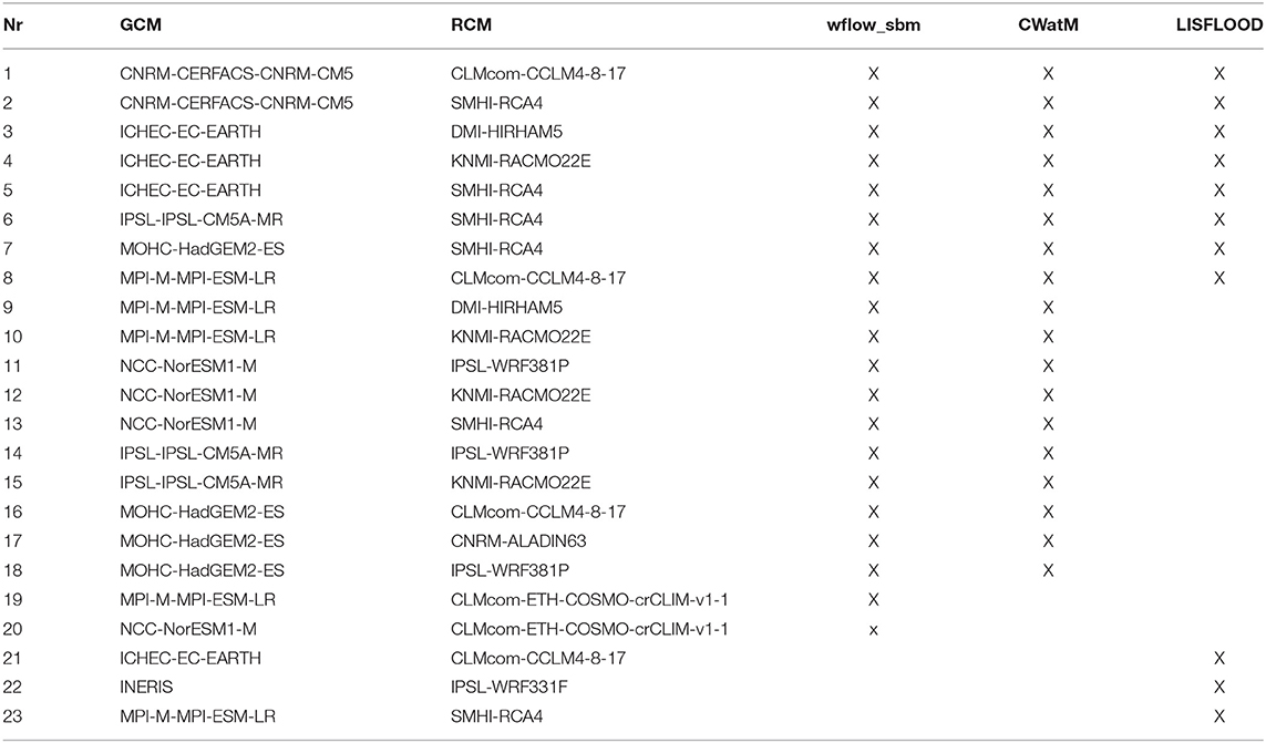
Table 2. Overview of CORDEX simulations available for the three hydrological models, the X indicates that the hydrological model was run with this CORDEX GCM-RCM combination.
Discharge Observations
Observed discharge time-series are used as historical reference. Most data are sourced from the Global Runoff Data Centre (GRDC), these are supplemented where needed with data from national providers; see Table 3.
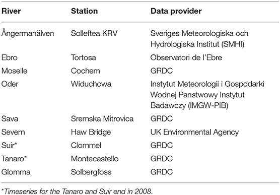
Table 3. Data sources and discharge stations of the historical reference data, locations are given in Figure 1.
Performance-Based Weighting
In search of optimizing the information content of the ensemble of simulations two different weighting methods (Kiesel et al., 2020) are selected to derive the weighted ensemble mean and reduce the ensemble spread. The resulting projections are shown next to the unweighted ensemble means.
Climate Model Weighting by Independence and Performance
The Climate model Weighting by Independence and Performance (ClimWIP) method (Sanderson et al., 2015a,b; Knutti et al., 2017; Lorenz et al., 2018; Brunner et al., 2019) accounts for the historical GCM performance of meteorological variables considered relevant for the correct representation of regional hydrology. In addition, it considers the independence of the individual GCMs, effectively down-weighting models which are identified as closely related to one another (Brunner et al., 2020; Merrifield et al., 2020). As a reference for the model performance the E-OBS dataset was used for the period 1980–2014. The point-to-point difference of the models to the observations determines the generalized model-observation distance Di and informs the performance weighting. The point-to-point difference between each model pair Sij informs the independence weighting. The combined weighting is defined as:
where the shape parameters σD controls the strength of the performance weighting and σS the strength of the interdependence weighting, and M is the number of model runs. Large values of σD lead to an approximation of equal weighting, while small values lead to aggressive weighting which can lead to overconfident results. For σS small values lead to all models being considered independent, while large values correspond to all models being considered dependent. Usually an internal perfect model test is used to estimate the parameters, however, due to the small ensemble this was not possible in this case. Therefore, the shape parameters were set manually with values similar to those used by Brunner et al. (2019) for Europe (σD = σS = 0.6).
The generalized model-observation distance Di can be based on any variable of the GCMs if observations are available. Here six diagnostics are used to inform the weights, as summarized in Table 4 similar to Lorenz et al. (2018). Increasing the number of diagnostics leads to convergence of the performance, while using too few can lead to overconfident estimates. The chosen variables include precipitation (pr), near-surface air temperature (tas) and surface downwelling shortwave radiation (rsds) which are all used as input for the hydrological modeling chain. For the derivation of the indicators the values were averaged over the given season and region given in the Table 4 (IPCC, 2012), which include the entire domain of Europe (EUR) and the Mediterranean (MED). A mask was applied to exclude sea area from the analysis. A schematic representation of the weighting method is given in Figure 2.
Table 4. Information on which the diagnostics used to calculate Di and Sij is based.
Figure 2. Schematic overview of the Climate model Weighting by Independence and Performance (ClimWIP) and Reliability Ensemble Averaging (REA) methods.
Reliability Ensemble Averaging
The second method is the Reliability Ensemble Averaging method (REA; Giorgi and Mearns, 2002) which we also applied in Sperna Weiland et al. (2012). This method considers the model bias (B) for the current climate (RB, i) from model number i and the GCM reliability in terms of the convergence of the GCM specific future discharge change with the weighted ensemble mean future change (RD, i) to calculate the overall GCM reliability factor, . In this study the climate data for the LISFLOOD simulations have been bias-corrected. Therefore, the first criterium, model bias for the current climate, cannot be assessed. The REA method is thus only applied to the CWatM and wflow_sbm simulations. The REA method is applied to the annual mean discharge at the discharge gauge stations in Table 3. The normalized reliability factor for mean discharge, , of the ith GCM-RCM combination is given by:
RB, i is a function of BQ, i, the bias of the ith GCM-RCM derived discharge from the gridded observed discharge, the higher the bias the lower the reliability factor. RD, i is a function of DQ, i, the distance of the discharge change calculated by the ith GCM from the REA ensemble average change. High reliability factors are only obtained when both the bias for the current climate and the distance to ensemble weighted future change are small compared to that of the other models. εQ is a measure of natural variability. To calculate εQ, 20-year moving averages are derived from the observed time-series and the difference between the minimum and maximum calculated moving average is assessed. The maximum length of the time-series used is 40 years to avoid the influence of trends. When the bias (BQ, i) or the distance to the weighted ensemble mean change (DQ, i) is smaller than the natural variability, the model reliability factor for bias or distance is set to 1. The exponents n and m in Equation (2) can be used to assign weights to the different criteria, however assignment of weights is mainly a subjective decision, therefore we set the value of both m and n to 1. The convergence or distance, DQ, i, can be calculated in an iterative process, where in a first step the distance of the individual GCM change, ΔQi, is calculated relative to the non-weighted ensemble mean change. From these distances reliability factors are then derived and a first weighted average change is calculated. In subsequent steps the deviations from the weighted average are used to derive new reliability factors until this process converges. The disadvantage of multiple iterations is that in case of large biases the method may highly favor only one or a few models.
Differences Between the Weighting Methods
The difference between the REA and ClimWIP method can be seen in Figure 2. The REA method focuses on discharges simulated by the hydrological models forced with CORDEX data (historical performance and projected change) whereas ClimWIP focuses on meteorological variables simulated by the GCMs (historical performance only). The end result of the ClimWIP method are the weights per GCM that are uniform for Europe. The end results of the REA method are for each GCM-RCM-hydrological model combination specific and vary between the different basins.
Results
Historical Discharge Regimes
The graphs in Figure 3 display the historical discharge regime for the period 1981–2010 as simulated by the three hydrological models (from left to right: wflow_sbm, CWatM, LISFLOOD) using the CORDEX datasets. As a reference the observed regime was plotted in black. For the wflow_sbm model the simulation of the historical meteorological data (E-OBS) was also added to the graph to get an impression of hydrological model vs. climate data bias. The color coding in all plots refer to the same CORDEX realizations, the ensemble mean is presented with a blue dotted line. The discharge regimes obtained with LISFLOOD show highest resemblance with the observed regime as this model has been calibrated and the CORDEX precipitation and temperature have been bias-corrected. This clearly reduces the spread between the discharges obtained from the different CORDEX datasets. On the other hand, the similarity between the CWatM and wflow_sbm simulations is large for most of the basins. The CORDEX simulations result in comparable discharge ranges.
Figure 3. Historical discharge regimes (m3 s-1) calculated over the period 1981–2010 from the CORDEX simulations (colored lines), the ensemble mean (blue dotted line) with from left to right (wflow_sbm, CWatM and LISFLOOD), observed discharge (black) and reference wflow_sbm run based on EOBS (dashed black). To refer to the CORDEX realizations the same color coding is used in all graphs.
The set of GCM-RCM combinations considered is almost the same for CWatM and wflow_sbm. For LISFLOOD the number of combinations is slightly less (11 vs. 20). This has likely also reduced the ensemble spread.
Overall for many rivers the LISFLOOD simulations resemble the observed (black line). Clear deviations can be found for the Ångermanälven. For many of the basins the wflow_sbm run forced with EOBS data (dashed black line, Figure 3) also resembles the observations and the LISFLOOD simulations. There are differences between the two models for the Glomma and Ångermanälven. This is partly caused by the reservoir representation in the wflow_sbm model, but possibly also influenced by the quality of the EOBS dataset in Northern regions where the gauge density is relatively low. For the Sava discharge simulated with wflow_sbm is continuously at least 500 m3s−1 lower than the observations. The CWatM model has not been explicitly calibrated for any of the nine catchments, instead CWatM was calibrated across the entire European domain based on a set of 363 observed discharge time series to obtain a unified set of model parameters. Most of the observed time series were located in Central Europe, thereby potentially leading to a biased representation of snowmelt processes in Northern Europe and evaporation in southern Europe. The wflow_sbm model has not been calibrated, however reservoirs and lakes have been added to the model based on the GRanD and HydroLakes datasets (Lehner et al., 2011; Messager et al., 2016). Solefteå KRV in the Ångermanälven is just below a hydropower plant which decreases the amplitude of the observed flow. The Glomma river discharge is influenced by several hydropower stations upstream as well. The relative high flow during summer can be a result of the RCM biases. According to Fantini et al. (2018) the EURO-CORDEX ensemble has a wet summer bias over Sweden and Norway. Many human managed reservoirs and dams are also located in the Ebro river. These highly influence the flow at Tortosa downstream in the Ebro basin. The human influences cannot be simulated well by the hydrological models.
The wflow_sbm run forced with E-OBS data resembles the observed flow well for many other basins. Thus, for most rivers the bias in simulated flow, i.e., the large overestimation, is predominantly caused by the bias in the CORDEX datasets and then specifically precipitation. This can be concluded from the difference between the flow simulations based on E-OBS and the flow simulations for the EURO-CORDEX ensemble. We also compared our results with past studies that evaluate EURO-CORDEX precipitation. According to Fantini et al. (2018) the CORDEX ensemble has a wet winter bias over France and a small wet annual mean bias over Northern Spain this possibly results in the overestimations of flow for the Moselle and Ebro. During summer there is a slight dry bias over France. The seasonal flow pattern is replicated well, but there is a large underestimation of the summer low flow probably due to an underestimation of the land-atmosphere interactions (e.g., convective) in summer by the RCMs (De Roo et al., 2016).
There is too little information to draw conclusions, but for the Glomma and Ångermanälven, the wflow_sbm simulations based on E-OBS resemble the LISFLOOD simulations more than the actual observations. This may be a result of the bias, or low presence of precipitation gauges, in the E-OBS data for Northern regions that influences the bias-correction of EURO-CORDEX for LISFLOOD and the quality of the EOBS driven wflow_sbm simulations.
For general performance evaluation of the individual hydrological models we refer to Imhoff et al. (2020) for wflow_sbm, Burek et al. (2020) and Greve et al. (2020) for CWatM and Arnal et al. (2019) for LISFLOOD.
Projected Discharge Changes
Tables 5–7 present the projected changes for the period 2031–2060 for RCP8p5 for three selected discharge statistics; 7-day annual minimum flow (Table 5), annual mean discharge (Table 6) and annual maximum flow (Table 7). All three statistics are averaged over the full period. Change is calculated relative to the period 1981–2010. The numbers 1–18 represent the different CORDEX GCM-RCM combinations listed in Table 2. For LISFLOOD projections are only available for combination 1–8. Changes for 7-day low flow are most pronounced and consistent between the models. Mainly decreases in low flows (see Table 5) are projected for the rivers in Southern Europe; the Tanaro and Ebro. Decreases in summer precipitation and increases in evaporation caused by rising temperatures decrease the low flow. For the Glomma and Ångermanälven in Scandinavia all model combinations project increases of the base flow. Increasing temperatures will lead to earlier snow melt, snow accumulation and melt processes currently highly influences the annual hydrological cycle. More precipitation will fall as rain. In addition, precipitation amounts will increase for Northern Europe leading to higher base flows. For the other rivers the signal is less pronounced. The LISFLOOD projections tend most toward decreases of flows, see for example the Severn and Suir. Although the modeling approach for LISFLOOD (hydrological model calibration and bias-correction of climate data) is different from the modeling approach for CWatM and wflow_sbm, there is no clear difference in projected changes except for the Moselle and Severn where the climate change signal is not very pronounced caused by the large uncertainty and variation in precipitation patterns.
Table 5. Projected change in long-term average 7-day minimum low flow between the periods 1981–2010 and 2031–2060.
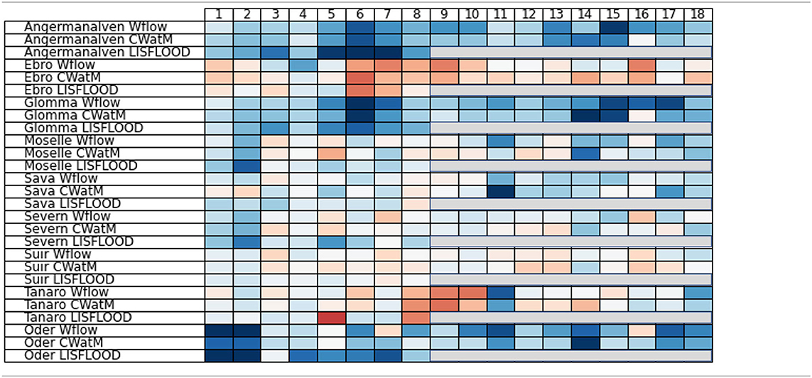
Table 6. Projected change in long-term average annual mean flow between the periods 1981–2010 and 2031–2060.
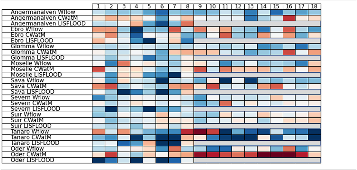
Table 7. Projected change in long-term average annual maximum flow between the periods 1981–2010 and 2031–2060.
This result indicates that the signal from the climate models is stronger than the possible influence of corrections. The changes projected for mean discharge are still relatively consistent between the models, yet smaller than the changes projected for low flows. For the Ångermanälven, Glomma and Oder average flow is projected to increase. For the Ebro and Tanaro decreases in mean discharge are most likely. For the other rivers the change signal is small and less consistent. Some indications of increased flow variability can be found with decrease in low flows and increases in high flows, as for example for the Sava and Suir according to LISFLOOD.
For long-term average maximum flow the change signal is very inconsistent both between the CORDEX simulations and between the hydrological models. Pronounced change signals can be found for an increase in maximum flow for the Ångermanälven with wflow_sbm and a decrease in maximum flow projected by CWatM for the Oder. Within a 30-year period there are often only a few extremes that are dampened by the natural climate variability. The period is too short to make a reliable estimate of in- or decreases of flood extremes.
Projected Changes - Diversity
Kiesel et al. (2020) propose several methods for model weighting and selection among which the “diversity of GCMs,” “diversity of RCMs,” and “diversity of hydrological models.” For example, for “diversity of GCMs,” this implies that from each GCM group the RCM model that best represents historic climate variability is selected. The idea of sub-selecting by choosing only one type of model (GCMs, RCMs or hydrological models) suggests that there would be largest consistency in projections for a single model from a given model type. Either the GCM, RCM or hydrological model would dominate the change signal. To verify this, the full set of changes projected per model are presented in the boxplots in Figure 4 for a selection of rivers (see the Supplementary Material for the remainder of rivers). Each boxplot represents all projections available for the specific hydrological model, RCM or GCM mentioned on the x-axis. Unfortunately, this number is not the same for all RCMs, GCMs and hydrological models and this also influences the width of the boxplots which thus only allow for a qualitative comparison. We selected the Ebro with a pronounced projected decrease of flow, the Ångermanälven with a pronounced increase in flow and the Moselle with a mixed change signal. Plots for the other rivers are given in the Supplementary Material. Focus is on the projected change in 7-day low flow because of the relative high consistency for this statistic.
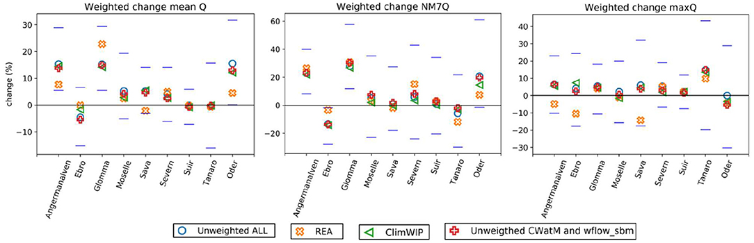
Figure 4. Boxplots representing the projected changes in 7-day low flow for from left to right, the 3 hydrologic models (green), the 7 GCMs (red), the 6 RCMs (blue) and the full set (cyaan). The spread of the boxplots is influenced by the number of available simulations and this number has therefore been added between brackets to the labels of the x-axis.
For all three rivers the boxplots represent large variation in the projections of a single model, independent of the model type (thus GCM, RCM or hydrological model). Related to the idea that the GCM signal dominates the change projection, we would have expected the red boxplots to be narrow compared to the other boxplots, but this is not the case. The spread of the MPI-MPI-ESM-LR set is relatively small for all three rivers, indicating that this GCM has a larger influence on the change signal than the RCM and hydrological model. The width of the boxplots for the LISFLOOD simulations is less than for the other hydrological models for many of the rivers. The main difference between the hydrological modeling chains is the application of bias-correction by the European Joint Research Center (JRC). This is a possible indication that the bias-correction does influence the change signal slightly. The inter-quantile ranges for CNRM-ALADIN63 and CLMcom-ETH-COSMO-crCLIM-v1-1 are small, yet only two simulations are available for these RCMs. Overall it can be concluded that the variation for a single model, either hydrological, RCM or GCM, is in a range similar to that of a random selection of realizations. Therefore, for this set of CORDEX simulations, we decided that the “diversity” based selection is not the preferred approach, information may be lost. In addition, all hydrological simulations were already available so there was no need to reduce the computation time by clustering.
Projected Changes - Performance Based Weighted Projected Changes
Two methods were applied to assess the influence of performance-based weighting and to derive more robust change signals. The first method, ClimWIP, is based on large scale performance for a set of GCM meteorological variables. This resulted in the weights listed in Table 8 for the driving GCMs. These weights were applied to all hydrological model realizations originating from the given GCM, normalized by dividing through the number of realizations for this GCM. This method includes changes assessed by all three hydrological models.
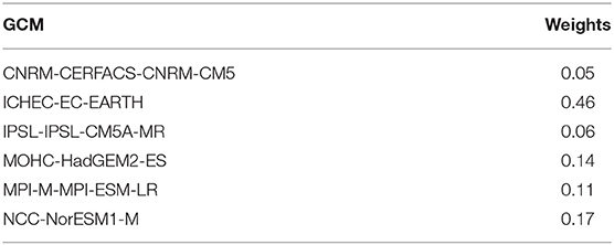
Table 8. Weights determined by the method of Brunner et al. (2019).
The second method, REA, was applied to all realizations available for CWatM and wflow_sbm. As mentioned before, LISFLOOD simulations were excluded from this weighting method as the GCM/RCM bias could not be assessed after the bias-correction applied to precipitation and temperature. Figure 5 displays the weights assigned to the different CORDEX-hydrological model combinations for the individual river basins. The sum of all weights for a single river basin equals 1. Both simulations with CWatM and wflow_sbm are assigned high weights, indicating that depending on the river either one model outperforms the other. Worth noticing are the relatively high weights assigned to the CORDEX combinations forced with the GCM ICHEC-EC-EARTH (nr 4 and 5), the GCM that was also assigned a high weight by the ClimWIP method. The REA method also assigns high weights to the CNRM-CERFACS-CNRM-CM5_SMHI-RCA4 CWatM simulation for several basins. Besides this there is a large variation in weights assigned for the different river basins. Often most model combinations receive a weight below 0.1, indicating that the REA weighted change signal is dominated by a few model combinations.
Figure 5. Weights calculated for the individual hydrological model-GCM-RCM combinations for the nine river basins (see legend). The numbers on the x-axis correspond to the GCM-RCM CORDEX datasets listed in Table 2. First all combinations for Wflow are given, second all combiations for CWatM. The sum off all weights for one river including both CWatM and Wflow simulations adds up to 1.
Figure 6 presents the resulting weighted changes in 7-day minimum, mean and annual maximum discharge together with the overall ensemble mean changes and the ensemble mean change from all wflow_sbm and CWatM realizations. The latter was added as a reference for the REA method. For most rivers the changes projected by (1) the full non-weighted ensemble, (2) the ClimWIP weighted ensemble and (3) the reduced ensemble existing of the CWatM and wflow_sbm realizations alone, are of the same order of magnitude. Mean projected changes are of the same order of magnitude and for some rivers the markers representing this change even overlap. The unweighted changes projected by the full ensemble are often slightly higher. For those rivers LISFLOOD provides higher increases. The REA method results in deviating changes. The main cause for this is the large bias for the historical period. All realizations are biased, highest weights are assigned to the least biased historical realizations and by iterating over the ensemble weighted changes the influence of the reliability factor for bias has a stronger influence on the outcome than the reliability factor for distance in future projected change. This is an indication that when these large biases and large variation therein exist, the biases dominate the REA method and the resulting weighted changes are less reliable. For some basins the influence is small, but for the Ångermanälven, Glomma, Sava and Oder the REA weighted change gets close to the uncertainty bands. The change signal for all discharge statistics in these basins obtained with the REA method deviate from the non-weighted ensemble projections and follow the change projected by the favored GCM(s). To reduce the influence of these single GCMs it was decided to iterate only once to assess the weighted change.
Figure 6. Projected future changes in annual mean discharge based on the full set of realizations - Unweighted ALL (blue), the Reliability Ensemble Averaging method – REA (orange), the realizations available for CWatM and LISFLOOD – Unweighted CWAtM, wflow_sbm (green) and ClimWIP (red) for the nine selected river basins. Together with the 5 and 95% uncertainty bounds of the full ensemble (blue dash).
The results of the ClimWIP method are more promising. The difference between the unweighted ensemble change and the change projected with the ClimWIP weighting method do not differ that much. While with the ClimWIP method 2 out of 6 models are assigned only a weight of ~5% and one model clearly dominates the rest (ICHEC-ECEARTH). This is the same GCM that received high weights from the REA method for several basins. This indicates that this model, that performs best compared to the other 5 GCMs when evaluated on large scale climate variables, also provides basin scale discharge projections that are in line with the projections obtained when the full ensemble is considered. This increases the confidence in both sets of projections. Slightly larger differences between the non-weighted change and ClimWIP method are found for the Oder and Ebro.
Discussion
In general, the projected discharge changes in this study are in line with previous studies (Dankers and Feyen, 2008; Blöschl et al., 2019). They indicate increases in flow for rivers in Scandinavia related to precipitation increases. Decreases of (low) flows are likely in Southern Europe and this urges the need for further adaptation to anticipate future severe droughts. For rivers in Central Europe the discharge change signal is more diverse, which is caused by the large natural variability and the absence of a strong climate change signal.
This study is based on a large set of existing hydrological model simulations. Consequently, there is a clear inconsistency in modeling chains; calibrated vs. uncalibrated, bias-correction vs. no bias-correction and the number of CORDEX simulations available differs per hydrological model. The results of this study should therefore be interpreted as indicative and some analyses are only based on part of the realizations. At the same time, these differences provided additional insights.
The hydrological simulations are based on the same CORDEX-RCM forcing, but all originate from different modeling efforts and therefore experimental differences exist. Wflow_sbm has only been calibrated for one parameter. CWatM has been parameterized based on a European wide optimization. For LISFLOOD dedicated basin scale calibration was applied. In addition, for the LISFLOOD runs the CORDEX temperature and precipitation have been bias-corrected. There are pros and cons in applying bias-correction. One of the disadvantages being its influence on the change signal (Themeßl et al., 2012; Cloke et al., 2013). Ideally, the experiment would be repeated using bias-corrected datasets for all the models to evaluate whether (1) this would result in similar projections and (2) to be able to make fully grounded statements on the relevance of the calibration and bias-correction for the climate projections for the different basins. Unfortunately, this is computationally too expensive and thus behind the scope of the current study. Nonetheless, even in the face of these inconsistencies, robust climate change signals emerge in Northern and Southern Europe, pointing toward high confidence in climate change impacts on average and extreme river flows in these regions.
Especially for the rivers with a pronounced change signal, the agreement in changes projected with the different hydrological models is large. Thus, the choice of the hydrological model used is not dominant. In addition, the fact that the LISFLOOD projections are in line with the other projections indicates that the influence of a bias-correction method on the projected change signal is not that strong. Although, overall changes obtained with LISFLOOD tend to be slightly higher. The differences between the models (parameterization, process description, calibration, bias-correction) become more pronounced in areas without a strong climate signal and larger natural climate variability. In future research this study could be extended. The set of hydrological simulations and models to be included should be set up-front. This will allow for fully transparent comparisons and evaluation of techniques.
For the current study the assumption is made that the hydrological model calibrations hold under changing future climate conditions. For wflow_sbm calibration is limited, however the parameters are based on catchment and soil properties that may also change in the future. It is behind the scope of the current study, but in further research it could be worth investigating for all three hydrological models whether the parameter values result in equal performance for relatively dry and relatively wet years from the historic record that may also occur under future climate conditions and the number of gauges used per catchment could be extended. Previous research has shown that an enhanced calibration approach that considers intermediate basin gauges, different climate conditions and where relevant glacier mass hold the potential to reduce uncertainties in the future hydrological projections (Huang et al., 2020; Ismail et al., 2020).
Analysis of the historical simulations clearly showed that the bias in simulated discharge was pre-dominantly a result of the bias in precipitation in the CORDEX simulations. Hydrological model simulations with observed meteorological data resulted in discharge regimes that highly resembled the observed discharge regime for most rivers and clearly outperformed the CORDEX driven hydrological simulations. This confirms that, when interested in absolute discharge values, bias-correction is recommended, or otherwise estimated relative changes should be applied to historical discharge observations.
One of the goals of this study was to reduce the uncertainty in the projections of future discharge changes. Kiesel et al. (2020) proposed two main ways to achieve this, either weighting or clustering. Within this study we were in the favorable position to have this large set of CORDEX based hydrological simulations at hand and there was no computational need for model sub-selection. In addition, the diversity analysis showed that the spread of realizations for any single GCM, RCM or hydrological model was comparable. The results did not confirm that within such a sub-set of our ensemble there would be more consistency than within the whole ensemble of realizations. Therefore, it was decided not to apply a clustering method, but instead focus on two weighting methods: ClimWIP and REA. ClimWIP highly favored one of the GCMs giving it almost half of the total weight. This is a much higher weight than the 1/6 of the weight it would have received in the equally weighted case. Still, the resulting weighted average ensemble mean change does not differ much from the non-weighted ensemble change for most rivers. This indicates that the ClimWIP model favors a GCM that performs well for large scale climate variable and that also provides basin scale discharge projections that are in line with the projections obtained when the full ensemble is considered. On the other hand, we have also seen from the high diversity between models shown in the boxplots per model that the GCM signal is not dominating the overall change projection and weighting on GCMs alone may not be sufficient. Finally, there are a few RCMs that are outside the inter-quantile-range of all models. Another method for optimizing or sub-selecting the ensemble could have been the exclusion of those.
Next to the ClimWIP method we applied the REA method to river discharges. The method focuses on historical bias and difference in projected changes for river discharge. Both having an equal importance. Unfortunately, in our case the bias in simulated historical discharge is large and diverse. For some rivers the final REA change can be highly dominated by a single GCM-hydrological model combination that has a relatively small bias. The three models have all been schematized based on best available (global) datasets, advanced hydrological model calibration could be a first step to reduce the influence of this bias. Another way of reducing the bias would be the correction of the climate data, however several past studies have indicated the influence of the bias-correction on the change signal in the climate data (Themeßl et al., 2012; Cloke et al., 2013).
In this study, for many rivers a single model was also assigned a weight of more than half the total weight. For the Ebro the result—nearly zero change in future annual average river discharge—was not in line with our expectations. This result comes from the fact that there was one model that clearly outperformed the other models for the historical periods and got a weight of more than 0.6. As discussed by Knutti et al. (2017) and Kiesel et al. (2020) the historically best performing model may not be the best in reproducing the climate change signal. To reduce this model's influence the number of iterations for the ensemble weighted change was already reduced to two. In addition, in future work, when one has significantly long observed time-series at hand for all basins, the REA method could be extended with a weight for the reproduction of observed historical trend (Sperna Weiland et al., 2012). This may be more relevant than the historical bias as it provides information on the reproduction of the change signal. Another possibility to improve the method would be adjusting the m and n factors of the two reliability criteria hereby decreasing the influence of the bias on the overall weight. Yet, the values to be used for m an n remain subjective. From the comparison between weighting methods it can be concluded that weighting climate models based on large scale climate patterns is more reliable than weighting on basin specific discharges. However, both methods favored similar GCMs.
This study is based on RCP8p5 which is a high-end scenario. It was selected because of its pronounced change signal. The projections are likely more severe than they would have been with scenarios usually selected for policy making purposes. Although there is large variation in the derived changes, overall the results do show some consistency. For most rivers there is a clear direction of change. In many cases, climate change exaggerates a problem that already exists like re-occurring severe droughts in Mediterranean countries. Here adaptation is needed and ongoing. In other cases, like the Moselle, the numbers indicate a need for further localized research to see for example whether we can expect further decreases in 7-day low flow that can hamper navigation in the future (Christodoulou et al., 2020).
Conclusion
Within this study we assessed the impact of climate change on river flow for nine basins spread over Europe with varying climate conditions and catchment characteristics using an ensemble EURO-CORDEX climate models and three hydrological models.
For two hydrological models we qualitatively evaluated the simulated historic flows. The LISFLOOD model forced with the with EOBS precipitation and temperature bias-corrected CORDEX data and the wflow_sbm model forced with EOBS data resemble observed flows reasonably well. Clear exceptions are the Scandinavian rivers Glomma and Ångermanälven, where performance is influenced by representation of reservoirs in the models and the low density of meteorological observations in the EOBS dataset. Both the wflow_sbm model and CWatM were run with the raw CORDEX data and for many rivers the thus simulated flows are comparable.
In line with existing work, the future projections indicate likely discharge decreases for the rivers in Southern Europe whereas increases are more likely for basins in Northern Europe. The large set of hydrological CORDEX based simulations we had available for three different hydrological models allowed to draw additional conclusions. The influence of the hydrological model, it's calibration and the application of bias-correction on projected discharge changes showed to be limited in basins with a strong climate change signal. Here, the climate signal dominates the projected direction of change. Yet, in central Europe where the changes are more variable the different model chains result in variable projections.
The consistency in the projected 7-day minimum flow statistic is highest, especially for Southern basins where evaporation will increase, summer precipitation may decrease and thus low flows will decrease. Projected changes in maximum flow are highly variable. There is clearly an uncertainty in projected maximum flow, caused by the large uncertainties in climate model precipitation. In addition, the 30-year time periods are too short to provide a representative set of annual maxima. Finally, estimates of peak flows are model dependent and rather sensitive to different routing and model parameterizations.
An analysis of the diversity in the projections showed that the variation for a single model, either GCM, RCM or hydrological model, is in a range similar to that of a random selection of realizations. Within the ensemble used here the GCM signal does not dominate the projection. Therefore, ensemble sub-selecting was not applied.
From the comparison between weighting methods it can be concluded that weighting climate models based on large scale climate patterns is more reliable than weighting on basin specific discharges. The REA method resulted in this study in very mixed and sometimes deviating change projections. However, both the REA and ClimWIP method favored simulations with ICHEC-EC-EARTH for at least part of the basins. The change in future projections, introduced by the weighting methods has a limited influence on the projected direction of change. However, the fact that a consistent change signal is obtained when either the full non-weighted ensemble or a weighted change where a single model dominates the change signal is used, increases the confidence in the projections.
Finally, some uncertainties and biases in the change signal cannot be resolved by applying bias correction or post-processing weighting techniques. There remains a need for both improved forcing data and model parameterization.
Data Availability Statement
The raw data supporting the conclusions of this article will be made available by the authors, without undue reservation.
Author Contributions
FS led the research and writing of the article. RV conducted the hydrological simulations for Wflow and the Wflow analysis. BB conducted the LISFLOOD simulations and contributed to the paper writing. PG conducted the CWatM simulations and contributed to the paper writing. LB contributed with the ClimWIP model weighting. AW contributed to the research design and paper writing. All authors contributed to the article and approved the submitted version.
Funding
This work has received funding from the EU Horizon 2020 Program for Research & Innovation, under grant agreement no 776613 (EUCP: EUropean Climate Prediction system; https://www.eucp-project.eu). The research was co-funded by the Deltares Strategic Research Program Natural Hazards.
Conflict of Interest
RV was employed by company Witteveen+Bos Consulting Engineers.
The remaining authors declare that the research was conducted in the absence of any commercial or financial relationships that could be construed as a potential conflict of interest.
Publisher's Note
All claims expressed in this article are solely those of the authors and do not necessarily represent those of their affiliated organizations, or those of the publisher, the editors and the reviewers. Any product that may be evaluated in this article, or claim that may be made by its manufacturer, is not guaranteed or endorsed by the publisher.
Acknowledgments
We thank the Sveriges Meteorologiska och Hydrologiska Institut (SMHI), Observatori de l'Ebre, Instytut Meteorologii I Gospodarki Wodnej Panstwowy Instytut Badawczy (IMGWPIB) and UK Environmental Agency for kindly providing the observed discharge time-series for, respectively, the Ångermanälven, Ebro, Oder, and Severn. All other data were obtained from the Global Runoff Data Centre, 56068 Koblenz, Germany.
Supplementary Material
The Supplementary Material for this article can be found online at: https://www.frontiersin.org/articles/10.3389/frwa.2021.713537/full#supplementary-material
Supplementary Figure 1. Boxplots representing the projected changes in 7-day low flow for the remainder of rivers not presented in Figure 4 for from left to right, the 3 hydrologic models, the 7 GCMs, the 6 RCMs and the full set. The spread of the boxplots is influenced by the number of available simulations and this number has therefore between brackets been added to the labels of the x-axis.
Supplementary Table 1. Projected change in long-term average 7-day minimum low flow between the periods 1981–2010 and 2031–2060. Similar to Table 5 but now sorted by model.
Supplementary Table 2. Projected change in long-term average annual mean flow between the periods 1981–2010 and 2031–2060. Similar to Table 6 but now sorted by model.
Supplementary Table 3. Projected change in long-term average annual maximum flow between the periods 1981–2010 and 2031–2060. Similar to Table 7 but now sorted by model.
References
Acreman, M., and Sinclair, C. (1986). Classification of drainage basins according to their physical characteristics; an application for flood frequency analysis in scotland. J. Hydrol. 84, 365–380. doi: 10.1016/0022-1694(86)90134-4
Alfieri, L., Burek, P., Feyen, L., and Forzieri, G. (2015). Global warming increases the frequency of river floods in Europe. Hydrol. Earth Syst. Sci. 19, 2247–2260. doi: 10.5194/hess-19-2247-2015
Arnal, L. S.-S, Asp, C., Baugh, A., de Roo, J., Disperati, F., Dottori, et al. (2019). EFAS Upgrade for the Extended Model Domain – Technical Documentation, EUR 29323 EN. Luxembourg: Publications Office of the European Union.
Baranzelli, C., Jacobs-Crisioni, C., Batista e Silva, F., Perpiña Castillo, C., Barbosa, A., Arevalo Torres, J., Lavalle, et al. (2014). The Reference Scenario in the LUISA Platform - Updated Configuration 2014 Towards a Common Baseline Scenario for EC Impact Assessment Procedures. Report EUR 27019 EN, Luxembourg: Publications office of the European Union.
Batista e Silva, F., Lavalle, C., and Koomen, E. (2013). A procedure to obtain a refined European land use/cover map. J. Land Use Sci. 8, 255–283. doi: 10.1080/1747423X.2012.667450
Beven, K. J., Wood, E. F., and Sivapalan, M. (1988). On hydrological heterogeneity—catchment morphology and catchment response. J. Hydrol. 100, 353–375. doi: 10.1016/0022-1694(88)90192-8
Bisselink, B., Bernhard, J., Gelati, E., Adamovic, M., Guenther, S., Mentaschi, L., et al. (2018). Impact of a Changing Climate, Land Use, and Water Usage on Europes Water Resources: A Model Simulation Study, EUR 29130 EN. Luxembourg: Publications Office of the European Union.
Blöschl, G., Hall, J., Viglione, A., Perdigao, R.A.P., Parajka, J., and Merz, B. (2019). Changing climate both increases and decreases European river floods. Nature 573, 108–111. doi: 10.1038/s41586-019-1495-6
Boé, J. (2018). Interdependency in multimodel climate projections: component replication and result similarity. Geophys. Res. Lett. 45, 2771–2779. doi: 10.1002/2017GL076829
Brunner, L., Lorenz, R., Zumwald, M., and Knutti, R. (2019). Quantifying uncertainty in european climate projections using combined performance-independence weighting. Env. Res. Lett. 14:124010. doi: 10.1088/1748-9326/ab492f
Brunner, L., Pendergrass, A. G., Lehner, F., Merrifield, A. L., Lorenz, R., and Knutti, R. (2020). Reduced global warming from CMIP6 projections when weighting models by performance and independence. Earth Syst. Dynam. 11, 995–1012. doi: 10.5194/esd-11-995-2020
Burek, P., Satoh, Y., Kahil, T., Tang, T., Greve, P., Smilovic, M., et al. (2020). Development of the community water model (CWatM v1.04) – a high-resolution hydrological model for global and regional assessment of integrated water resources management. Geosci. Model Dev. 13, 3267–3298, doi: 10.5194/gmd-13-3267-2020
Burek, P., van der Knijff, J. M., and De Roo, A. (2013). A: LISFLOOD: Distributed Water Balance and Flood Simulation Model, JRC Technical Reports, EUR 26162 EN. Luxembourg: Publications Office of the European Union, 142p.
Burek, P., Satoh, Y., Kahil, T., Tang, T., Greve, P., Smilovic, M., et al. (2021). Community Water Model (CWatM v1.04). Vienna: Zenodo.
Capros, P., Van Regemorter, D., Paroussos, L., Karkatsoulis, P., Fragkiadakis, C., Tsani, S., et al. (2013). GEM-E3 Model Documentation. Publications Office of the European Union. Available online at: https://publications.jrc.ec.europa.eu/repository/handle/111111111/32366 (accessed September 16, 2021).
Christodoulou, A., Christidis, P., and Bisselink, B. (2020). Forecasting the impacts of climate change on inland waterways. Transport. Res. Part D Transport Environ. 82:102159. doi: 10.1016/j.trd.2019.10.012
Clark, M.P., Wilby, R.L., Gutmann, E.D., Vano, J.A., Gangopadhyay, S., Wood, A.W., et al. (2016). Characterizing uncertainty of the hydrologic impacts of climate change. Curr. Clim. Change Rep. 2, 55–64. doi: 10.1007/s40641-016-0034-x
Cloke, H.L., Wetterhall, F., He, Y., Freer, J.E., and Pappenberger, F. (2013). Modelling climate impact on floods with ensemble climate projections. Q. J. R. Meteorol. Soc. 139, 282–297. doi: 10.1002/qj.1998
Cornes, R., van der Schrier, G., van den Besselaar, E.J.M., and Jones, P.D. (2018). An ensemble version of the E-OBS temperature and precipitation datasets. J. Geophys. Res. Atmos. 123, 9391–9409. doi: 10.1029/2017JD028200
Dankers, R., and Feyen, L. (2008). Climate change impact on flood hazard in europe: An assessment based on high resolution climate simulations. J. Geophys. Res. Atm. 113:D19105. doi: 10.1029/2007JD009719
De Bruin, H.A.R. (1983). A model for the Priestley-Taylor parameter α. J Clim. Appl. Meteorol. 22, 572–578. doi: 10.1175/1520-0450(1983)022<0572:AMFTPT>2.0.CO;2
De Roo, A., Bisselink, B., Beck, H., Bernhard, J., Burek, P., Reynaud, A., et al. (2016). Modelling Water Demand and Availability Scenarios for Current and Future Land Use and Climate in the Sava River Basin. Luxembourg: Publications Office of the European Union; EUR 27701 EN.
De Roo, A. P. J., Wesseling, C. G., and Van Deursen, W. P. A. (2000). Physically-based river basin modelling within a GIS: The LISFLOOD model. Hydrol. Process. 14, 1981–1992.
Deb, K., Pratap, A., Agarwal, S., and Meyarivan, T. (2002). A fast and elitist multiobjective genetic algorithm: NSGA-II. IEEE Trans. Evol. Comput. 6, 182–197. doi: 10.1109/4235.996017
Dosio, A., and Paruolo, P. (2011). Bias correction of the ENSEMBLES high-resolution climate change projections for use by impact models: Evaluation on the present climate. J. Geophys. Res. Atmos. 116:D16106. doi: 10.1029/2011JD015934
Dosio, A., Paruolo, P., and Rojas, R. (2012). Bias correction of the ENSEMBLES high resolution climate change projections for use by impact models: Analysis of the climate change signal. J. Geophys. Res. Atmos. 117:D17110. doi: 10.1029/2012JD017968
Eilander, D., van Verseveld, W., Yamazaki, D., Weerts, A., Winsemius, H. C., and Ward, P. J. (2021). A hydrography upscaling method for scale invariant parametrization of distributed hydrological models. Hydrol. Earth Syst. Sci. Discuss. 25, 5287–5313. doi: 10.5194/hess-25-5287-2021
European Commission (2014). “The 2015 ageing report. underlying assumptions and projection methodologies,” in: European Economy 8/2014. European Commission.
Eyring, V., Cox, P.M., Flato, G.M., Gleckler, P.J., Abramowitz, G., Caldwell, P., et al. (2019). Taking climate model evaluation to the next level. Nat. Clim. Change 9, 102–110. doi: 10.1038/s41558-018-0355-y
Fantini, A., Raffaele, F., Torma, C., Bacer, S., Coppola, E., Giorgi, F., et al. (2018). Assessment of multiple daily precipitation statistics in ERA-Interim driven Med-CORDEX and EURO-CORDEX experiments against high resolution observations. Clim. Dyn. 51, 877–900. doi: 10.1007/s00382-016-3453-4
Fortin, F. A., Rainville, F. M. D., Gardner, M. A., Parizeau, M., and Gagné, C. (2012). DEAP: Evolutionary algorithms made easy. J. Mach. Learn. Res. 13, 2171–2175.
Forzieri, G., Feyen, L., Russo, S., Vousdoukas, M., Alfieri, L., Outten, S., et al. (2016). A. Multi-hazard assessment in Europe under climate change. Clim. Chang. 137, 105–119. doi: 10.1007/s10584-016-1661-x
Gash, J. H. C. (1979). An analytical model of rainfall interception by forests. Q. J. R. Meteorol. Soc. 105, 43–55. doi: 10.1002/qj.49710544304
Giorgi, F., and Coppola, E. (2007). European climate-change oscillation (ECO). Geophys. Res. Lett. 34:L21703. doi: 10.1029/2007GL031223
Giorgi, F., and Mearns, L. O. (2002). Calculation of average, uncertainty range, and reliability of regional climate changes from AOGCM simulations via the “Reliability Ensemble Averaging” (REA) Method. J. Clim. 15, 1141–1158. doi: 10.1175/1520-442(2002)015<1141:COAURA>2.0.CO;2
Greve, P., Burek, P., and Wada, Y. (2020). Using the Budyko Framework for calibrating a global hydrological model. Water Res. Res. 56:e2019WR026280. doi: 10.1029/2019WR026280
Greve, P., Gudmundsson, L., and Seneviratne, S. I. (2018). Regional scaling of annual mean precipitation and water availability with global temperature change. Earth Syst. Dynam. 9, 227–240. doi: 10.5194/esd-9-227-2018
Gudmundsson, L., Seneviratne, S.I., and Zhang, X. (2017). Anthropogenic climate change detected in European renewable freshwater resources. Nat. Clim. Change 7, 813–816. doi: 10.1038/nclimate3416
Gupta, H. V., Kling, H., Yilmaz, K. K., and Martinez, G. F. (2009). Decomposition of the mean squared error and NSE performance criteria: Implications for improving hydrological modeling. J. Hydrol. 377, 80–91. doi: 10.1016/j.jhydrol.2009.08.003
Haddeland, I., Clark, D. B., Franssen, W., Ludwig, F., Voß, F., Arnell, N. W., et al. (2011). Multimodel estimate of the global terrestrial water balance: setup and first results. J. Hydrometeorol. 12, 869–884. doi: 10.1175/2011JHM1324.1
Havik, K., Mc Morrow, K., Orlandi, F., Planas, C., Raciborski, R., Röger, W., et al. (2014). “The production function methodology for calculating potential growth rates & output gaps,” in European Economy, Economic Papers, 535.
Hirpa, F. A., Salamon, P., Beck, H. E., Lorini, V., Alfieri, L., Zsoter, E., et al. (2018). Calibration of the global flood awareness system (GloFAS) using daily streamflow data. J. Hydrol. 566, 595–606. doi: 10.1016/j.jhydrol.2018.09.052
Huang, S., Shah, H., Naz, B.S., Shrestha, N., Mishra, P., Ghimire, U., et al. (2020). Impacts of hydrological model calibration on projected hydrological changes under climate change—a multi-model assessment in three large river basins. Clim. Change 163, 1143–1164. doi: 10.1007/s10584-020-02872-6
Imhoff, R. O., van Verseveld, W. J., van Osnabrugge, B., and Weerts, A. H. (2020). Scaling point-scale (pedo)transfer functions to seamless large-domain parameter estimates for high-resolution distributed hydrologic modeling: an example for the Rhine River. Water Res. Res. 56:e2019WR026807. doi: 10.1029/2019WR026807
IPCC (2012). “Summary for policymakers,” in Managing the Risks of Extreme Events and Disasters to Advance Climate Change Adaptation, eds C. B. Field, V. Barros, T. F. Stocker, D. Qin, D. J. Dokken, K. L. Ebi, et al. A Special Report of Working Groups I and II of the Intergovernmental Panel on Climate Change. (Cambridge; New York, NY: Cambridge University Press), 1–19.
Ismail, M. F., Naz, B. S., Wortmann, M., Disse, M., Bowling, L. C., and Bogacki, W. (2020). Comparison of two model calibration approaches and their influence on future projections under climate change in the Upper Indus Basin. Clim. Change 163, 1227–1246. doi: 10.1007/s10584-020-02902-3
Jacob, D., Petersen, J., Eggert, B., Alias, A., Christensen, O. B., Bouwer, L. M., et al. (2014). EURO-CORDEX: new high-resolution climate change projections for European impact research. Reg. Environ. Change 14, 563–578. doi: 10.1007/s10113-013-0499-2
Jacobs-Crisioni, C., Diogo, V., Perpina Castillo, C., Baranzelli, C., and Batista e Silva, F. (2017). The LUISA Territorial Reference Scenario 2017: A Technical Description. Publications Office of the European Union. Available online at: https://ec.europa.eu/jrc/en/publication/luisa-territorial-reference-scenario-2017 (accessed September 16, 2021).
Keramidas, K., Kitous, A., Després, J., Schmitz, A., Diaz Vazquez, A., Mima, S., et al. (2017). POLES-JRC Model Documentation. EUR 28728 EN. Luxembourg: Publications Office of the European Union. doi: 10.2760/225347
Kiesel, J., Gericke, A., Rathjens, H., Wetzig, A., Kakouei, K., Jähnig, S.C., et al. (2019). Climate change impacts on ecologically relevant hydrological indicators in three catchments in three European ecoregions. Ecol. Eng. 127, 404–416. doi: 10.1016/j.ecoleng.2018.12.019
Kiesel, J., Stanzel, P., Kling, H., Fohrer, N., Jähnig, S.C., and Pechlivanidis, I. (2020). Streamflow-based evaluation of climate model sub-selection methods. Clim. Change 163, 1267–1285. doi: 10.1007/s10584-020-02854-8
Kling, H., Fuchs, M., and Paulin, M. (2012). Runoff conditions in the upper Danube basin under an ensemble of climate change scenarios. J. Hydrol. 424–425, 264–277. doi: 10.1016/j.jhydrol.2012.01.011
Knutti, R., Sedlácek, J., Sanderson, B. M., Lorenz, R., Fischer, E. M., and Eyring, V. (2017). A climate model projection weighting scheme accounting for performance and interdependence. Geophys. Res. Lett. 44, 1909–1918. doi: 10.1002/2016GL072012
Kreibich, H., van den Bergh, J.C.J.M., Bouwer, L.M., Bubeck, P., Ciavola, P., Green, C., et al. (2014). Costing natural hazards. Nat. Clim. Chang. 4, 303–306. doi: 10.1038/nclimate2182
Kundzewicz, Z.W., Krysanova, V., Dankers, R., Hirabayashi, Y., Kanae, S., and Hattermann, F.F. (2017). Differences in flood hazard projections in Europe – their causes and consequences for decision making. Hydrol. Sci. J. 62, 1–14. doi: 10.1080/02626667.2016.1241398
Lavalle, C., Baranzelli, C., Batista e Silva, F., Mubareka, S., Rocha Gomes, C., Koomen, E., et al. (2011). “A high resolution land use/cover modelling framework for Europe,” in ICCSA 2011, Part I, LNCS 6782, 60–75.
Lehner, B., Reidy Liermann, C., Revenga, C., Vörösmarty, C., Fekete, B., Crouzet, P., et al. (2011). High-resolution mapping of the world's reservoirs and dams for sustainable river-flow management. Front. Ecol. Environ. 9, 494–502. doi: 10.1890/100125
Lorenz, R., Herger, N., Sedlácek, J., Eyring, V., Fischer, E. M., and Knutti, R. (2018). Prospects and caveats of weighting climate models for summer maximum temperature projections over north america. J. Geophys. Res. Atm. 123, 4509–4526. doi: 10.1029/2017JD027992
Melsen, L. A., Addor, N., Mizukami, N., Newman, A. J., Torfs, P. J. J. F., and Clark, M. P. (2018). Mapping (dis)agreement in hydrologic projections. Hydrol. Earth Syst. Sci. 22, 1775–1791. doi: 10.5194/hess-22-1775-2018
Merrifield, A. L., Brunner, L., Lorenz, R., Medhaug, I., and Knutti, R. (2020). An investigation of weighting schemes suitable for incorporating large ensembles into multi-model ensembles. Earth Syst. Dynam. 11, 807–834. doi: 10.5194/esd-11-807-2020
Messager, M.L., Lehner, B., Grill, G., Nedeva, I., and Schmitt, O. (2016). Estimating the volume and age of water stored in global lakes using a geo-statistical approach. Nat. Comm. 7:13603. doi: 10.1038/ncomms13603
Moriasi, D. N., Arnold, J. G., Van Liew, M. W., Bingner, R. L., Harmel, R. D., and Veith, T. L. (2007). Model evaluation guidelines for systematic quantification of accuracy in watershed simulations. Trans. ASABE 50, 885–900. doi: 10.13031/2013.23153
Ntegeka, V., Salamon, P., Gomes, G., Sint, H., Lorini, V., Thielen Del Pozo, J., and Zambrano, H. (2013). EFAS-Meteo: A European Daily High-Resolution Gridded Meteorological data Set for 1990 - 2011. EUR 26408. Luxembourg: Publications Office of the European Union. JRC86388.
Pennell, C., and Reichler, T. (2011). On the effective number of climate models. J. Clim. 24, 2358–2367. doi: 10.1175/2010JCLI3814.1
Piani, C., Weedon, G. P., Best, M., Gomes, S. M., Viterbo, P., Hagemann, S., et al. (2010). Statistical bias correction of global simulated daily precipitation and temperature for the application of hydrological models. J. Hydrol. 395, 199–215. doi: 10.1016/j.jhydrol.2010.10.024
Pokhrel, Y., Felfelani, F., Satoh, Y., Boulange, J., Burek, P., Gädeke, A., et al. (2021). Global terrestrial water storage and drought severity under climate change. Nat. Clim. Chang. 11, 226–233. doi: 10.1038/s41558-020-00972-w
Rutter, A.J., Kershaw, K.A., Robins, P.C., and Morton, A.J. (1971). A predictive model of rainfall interception in forests, 1. Derivation of the model from observations in a plantation of Corsican pine. Agr. Meteorol. 9, 367–384. doi: 10.1016/0002-1571(71)90034-3
Sanderson, B. M., Knutti, R., and Caldwell, P. (2015a). A representative democracy to reduce interdependency in a multimodel ensemble. J. Clim. 28, 5171–5194. doi: 10.1175/JCLI-D-14-00362.1
Sanderson, B. M., Knutti, R., and Caldwell, P. (2015b). Addressing interdependency in a multimodel ensemble by interpolation of model properties. J. Clim. 28, 5150–5170. doi: 10.1175/JCLI-D-14-00361.1
Sperna Weiland, F.C., van Beek, L.P.H., Weerts, A.H., and Bierkens, M.F.P. (2012). Extracting information from an ensemble of GCMs to reliably assess future global runoff change. J. Hydrol. 412–413, 66-75. doi: 10.1016/j.jhydrol.2011.03.047
Stahl, K., Hisdal, H., Hannaford, J., Tallaksen, L. M., Van Lanen, H. A. J., Sauquet, E., et al. (2010). Streamflow trends in Europe: evidence from a dataset of near-natural catchments. Hydrol. Earth Syst. Sci. 14, 2367–2382. doi: 10.5194/hess-14-2367-2010
Themeßl, M.J., Gobiet, A., and Heinrich, G. (2012). Empirical-statistical downscaling and error correction of regional climate models and its impact on the climate change signal. Clim. Change 112, 449–468. doi: 10.1007/s10584-011-0224-4
Thober, S., Rohini, K., Wanders, N., Marx, A., Pan, M., and Rakovec, O. (2018). Multi-model ensemble projections of european river floods and high flows at 1.5, 2, and 3 degrees global warming. Env. Res. Lett. 13:014003. doi: 10.1088/1748-9326/aa9e35
Todini, E., and Ciarapica, L. (2002). “The TOPKAPI model,” in Mathematical models of large watershed hydrology, eds V. P. Singh, and D. K. Frevert (Littleton, CO: Water Resources), 471–506.
Van Der Knijff, J. M., Younis, J., and De Roo, A.P.J. (2010). LISFLOOD: a GIS-based distributed model for river basin scale water balance and flood simulation. Int. J. Geogr. Inf. Sci. 24, 189–212. doi: 10.1080/13658810802549154
Keywords: ensemble projections, performance-based weighting, EURO-CORDEX, climate change, hydrological impact, Europe
Citation: Sperna Weiland FC, Visser RD, Greve P, Bisselink B, Brunner L and Weerts AH (2021) Estimating Regionalized Hydrological Impacts of Climate Change Over Europe by Performance-Based Weighting of CORDEX Projections. Front. Water 3:713537. doi: 10.3389/frwa.2021.713537
Received: 23 May 2021; Accepted: 04 October 2021;
Published: 10 November 2021.
Edited by:
Fuqiang Tian, Tsinghua University, ChinaReviewed by:
Kristian Förster, Leibniz University Hannover, GermanyRui Tong, Vienna University of Technology, Austria
Copyright © 2021 Sperna Weiland, Visser, Greve, Bisselink, Brunner and Weerts. This is an open-access article distributed under the terms of the Creative Commons Attribution License (CC BY). The use, distribution or reproduction in other forums is permitted, provided the original author(s) and the copyright owner(s) are credited and that the original publication in this journal is cited, in accordance with accepted academic practice. No use, distribution or reproduction is permitted which does not comply with these terms.
*Correspondence: Frederiek C. Sperna Weiland, ZnJlZGVyaWVrLnNwZXJuYUBkZWx0YXJlcy5ubA==