The acoustic Dirac equation as a model of topological insulators

The dynamical equations of motion for a discrete, one-dimensional harmonic chain with side restoring forces are analogous to the relativistic Klein–Gordon equation. Dirac factorization of the discrete Klein–Gordon equation introduces two equations with time reversal (T) and parity (P) symmetry-breaking conditions. The Dirac-factored equations enable the exploration of the properties of the solutions of the dynamic equations under PT symmetry-breaking conditions. The spinor solutions of the Dirac factored equations describe two types of acoustic waves: one with a conventional topology (Berry phase equal to 0) and the other with a non-conventional topology (Berry phase of π). In the latter case, the acoustic wave is isomorphic to the quantum spin of an electron, also known as an “acoustic pseudospin,” which requires a closed path, corresponding to two Brillouin zones (BZs), to restore the original spinor. We also investigate the topology of evanescent waves supported by the Dirac-factored equations. The interface between topologically conventional and non-conventional chains exhibits topological surface states. The Dirac-factored equations of motion of the one-dimensional harmonic chain with side springs can serve as a model for the investigation of the properties of acoustic topological insulators.

1 Introduction

A topological insulator cannot be adiabatically transformed into an ordinary insulator without passing through an intermediate conducting state (Qi and Zhang, 2011). While the bulk system is insulating, the surface can support conduction that is topologically protected, meaning that the surface states are insensitive to local perturbations (Hasan and Kane, 2010). Topological insulators can exhibit quantum mechanical properties such as the quantum spin Hall (QSH) effect (Qi and Zhang, 2010) and the anomalous quantum Hall (QH) effect, which occurs in the absence of an external magnetic field due to the breaking of time-reversal symmetry (Chang et al., 2023). Acoustic analogs of the QSH effect have been implemented (a) by tuning an accidental double Dirac cone in graphene-like lattices (He et al., 2016; Mei et al., 2016) and (b) via a BZ folding mechanism (Zhang et al., 2017; Yves et al., 2017; Xia et al., 2017; Deng et al., 2017). QH-related effects have been realized in acoustics by arranging circulating flows into periodic settings to form an acoustic lattice that breaks time reversal symmetry (Yang et al., 2015; Ni et al., 2015; Khanikaev et al., 2015).

Phononic structures can support elastic waves with non-conventional topology by breaking symmetry (Xue et al., 2022). Dirac factorization of the wave equation reveals potential topological properties that may result from symmetry breaking (which might be brought about by structural or external perturbations). For instance, the equations of motion of two coupled one-dimensional harmonic systems (Deymier and Runge, 2016) can be factored in the long wavelength limit as a product of two Dirac-like equations, each of which breaks parity symmetry and time reversal symmetry. Propagative wave solutions to each Dirac equation can satisfy two possible dispersion relations, giving rise to symmetric and anti-symmetric eigenmodes. The former exhibit the conventional character of Boson-like phonons, while the latter exhibit Fermion-like behavior of phonons (Deymier et al., 2015; Deymier et al., 2014). The topological properties of evanescent waves in product parity-time symmetry have also been investigated near exceptional points (Chen et al., 2024).

The wave equation for a two-dimensional plate coupled to a rigid substrate can also be subject to Dirac factorization (Deymier and Runge, 2022). These factors are analogous to the long-wavelength limit of the Qi, Wu, and Zhang (QWZ) model of the anomalous quantum Hall effect (Qi et al., 2006). The Dirac factorization reveals waves with spin-like degrees of freedom that have a gapped band structure, which is similar to the spin Hall effect. Kane and Lubensky (2014) demonstrate a method inspired by the Dirac factorization of the Klein–Gordon equation to establish a connection between topological mechanical modes and the topological band theory in electronic systems. This leads to the prediction of new topological bulk mechanical phases with distinct boundary modes. Topological phonons can also be classified using local symmetries (Süsstrunk and Huber, 2016) by adapting the classification of non-interacting electron systems to mechanical systems.

Here, we study solutions of the Dirac factorizations of the discrete one-dimensional harmonic chain with side restoring forces and investigate the appearance of edge modes at the interface of conventional and non-conventional topologies. In Section 2, we introduce the Dirac factorization of the discrete Klein–Gordon equation, and in Section 3, we find the dispersion relation and amplitude vectors corresponding to propagative wave solutions of the Dirac equations. Section 4 addresses evanescent wave solutions and their dispersion relation. In Sections 5 and 6, we compute the respective Berry phases of the amplitude vectors of the propagative and evanescent waves. Section 7 addresses the existence of edge modes at the interface between two topologically different semi-infinite media that obey the acoustic Dirac equation. Finally, in Section 8, we summarize and draw conclusions.

2 Model system and equation of motion for the discrete harmonic chain

We consider the model of the one-dimensional harmonic chain illustrated in Figure 1. We assume that the chain lies along the $x$-axis. The chain is composed of identical masses, $M$, interacting with their neighbors via linear spring forces with a spring constant $K$; each of the masses is connected to a rigid substrate through harmonic springs with a spring constant $K^{\prime }$. The coordinates of the $n^{th}$ mass at rest are $x_{0n}=na$, where $a$ is the spacing between adjacent masses at rest.

Figure 1

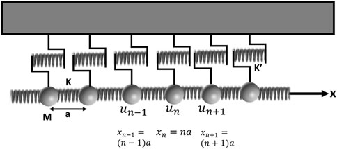
Figure 1. Schematic illustration of the one-dimensional harmonic chain attached elastically to a rigid substrate (top gray box). The side springs restore longitudinal motion.

We denote the displacement of the $n^{th}$ mass by $u_n=x_n-x_{0n}$. Newton’s equation for the $n^{th}$ mass is

$M\frac{d^2{u}_n}{{dt}^2}=K\left(u_{n+1}-u_n\right)-K\left(u_n-u_{n-1}\right)-K^{\prime }{u}_n(1)$

Taking ${\beta }^2=\frac{K}{M}$ and ${\alpha }^2=\frac{K^{\prime }}{M}$ in Equation 1, we can rewrite the above equation as

$\frac{d^2{u}_n}{{dt}^2}-{\beta }^2\left(u_{n+1}-2u_n+u_{n-1}\right)+{\alpha }^2{u}_n=0(2)$

The quantity $u_{n+1}-2u_n+u_{n-1}$ can be identified as a discrete second derivative with respect to position. Thus, Equation 2 can be thought of as a discrete version of the Klein–Gordon equation $\frac{{\partial }^{2}u}{\partial t^2}-{\beta }^2\frac{{\partial }^{2}u}{\partial x^2}+{\alpha }^{2}u=0.$ It can be shown that the continuous Klein–Gordon equation (when interpreted as an operator acting on vectors with two components) can be factorized as a product of Dirac equations:

$\left[{\sigma }_1\frac{\partial }{\partial t}\pm i\beta {\sigma }_2\frac{\partial }{\partial x}-i\alpha I\right]\left[{\sigma }_1\frac{\partial }{\partial t}\pm i\beta {\sigma }_2\frac{\partial }{\partial x}+i\alpha I\right]=I\frac{{\partial }^{2}u}{\partial t^2}-{\beta }^{2}I\frac{{\partial }^{2}u}{\partial x^2}+{\alpha }^{2}I(3)$

—where ${\sigma }_1=\left(\begin{array}{cc}0& 1\\ 1& 0\end{array}\right)$, and ${\sigma }_2=\left(\begin{array}{cc}0& -i\\ i& 0\end{array}\right)$ are the Pauli matrices and $I$ is the 2 × 2 identity matrix (Deymier and Runge, 2016).

Now, let us provide a physical interpretation of amplitude vectors with two components. We note that if $\alpha =0$, the equation corresponding to the first operator in the square bracket of Equation 3 becomes $\left[{\sigma }_1\frac{\partial }{\partial t}\pm i\beta {\sigma }_2\frac{\partial }{\partial x}\right]\psi =0$. Using a plane wave solution with $\psi =\left(\begin{array}{c}{a}_1\\ a_2\end{array}\right){e^{ikx}e}^{i\omega t}$, this equation reduces to the system $\left\{\begin{array}{c}\left(\omega \pm \beta k\right)a_2=0\\ \left(\omega \mp \beta k\right)a_1=0\end{array}\right.$. We obtain two solutions for the angular velocity of the plane wave $\omega =\pm \beta kh$. These correspond to plane waves propagating in the positive and negative directions. In this case, the components $a_1$ and $a_2$ are now independent of each other and of the wave number. The amplitude of the plane wave propagating in the positive direction is independent of that of the wave propagating in the opposite direction. When $\alpha \ne 0$, the plane wave solutions of the equation $\left[{\sigma }_1\frac{\partial }{\partial t}\pm i\beta {\sigma }_2\frac{\partial }{\partial x}-i\alpha I\right]\psi =0$ obey the system of linear equations $\left\{\begin{array}{l}\left(\omega \pm \beta k\right)a_2-\alpha a_1=0\\ \left(\omega \mp \beta k\right)a_1-\alpha a_2=0\end{array}\right.$ with the dispersion relation $\omega =\pm \sqrt{{\left(\beta k\right)}^2+{\alpha }^2}$. The amplitude components $a_1$ and $a_2$ are given by $\left(\begin{array}{c}{a}_1\\ a_2\end{array}\right)\propto \left(\begin{array}{c}\sqrt{\omega \pm \beta k}\\ \sqrt{\omega \mp \beta k}\end{array}\right)$. The components of the $2$ × $1$ amplitude vector are not independent of each other. This indicates that the directions of propagation are not independent of each other anymore; it is parameter $\alpha$ that couples those directions. The wave function $\psi$ has the character of quasi-standing waves, which are composed of forward and backward waves with a very specific proportion of their respective amplitudes $a_1$ and $a_2$.

In order to achieve a factorization of the discrete Klein–Gordon equation as a product of Dirac-like equations, we will interpret the operator $\frac{d^2}{{dt}^2}-{\beta }^2\left({\Delta }^{+}{\Delta }^{-}\right)+{\alpha }^2$ as acting on vectors with four components. Here, ${\Delta }^{+}$ is the forward difference operator defined by ${{\Delta }^{+}u}_n=u_{n+1}-u_n$, and ${\Delta }^{-}$ is the backward difference operator defined by ${{\Delta }^{-}u}_n=u_n-u_{n-1}$. These difference operators are linear (note that ${\Delta }^{+}{\Delta }^{-}{u}_n={\Delta }^{+}\left(u_n-u_{n-1}\right)={\Delta }^{+}{u}_n-{\Delta }^{+}{u}_{n-1}=u_{n+1}-2u_n+u_{n-1}$). The operators ${\Delta }^{+}$ and ${\Delta }^{-}$ can also be interpreted as operators on vectors where the difference operations are carried out component-wise.

Let $e_1=\left(\begin{array}{cc}0& 1\\ 0& 0\end{array}\right)$ and $e_2=\left(\begin{array}{cc}0& 0\\ 1& 0\end{array}\right).$ We can reformulate Equation 2 in terms of a product of two operators:

$\left[{\sigma }_1⨂I\frac{\partial }{\partial t}+i\beta {\sigma }_2⨂\left\{e_1{∆}^{+}+e_2{∆}^{-}\right\}+i\alpha I⨂I\right]\left[{\sigma }_1⨂I\frac{\partial }{\partial t}+i\beta {\sigma }_2⨂\left\{e_1{∆}^{+}+e_2{∆}^{-}\right\}-i\alpha I⨂I\right]$

It can be verified that this product is the same as $\mathit{I}\frac{{\partial }^2}{{\partial t}^2}-\mathit{I}{\beta }^2{∆}^{+}{∆}^{-}+{\alpha }^2\mathit{I}$ (with $\mathit{I}$ being the 4 × 4 identity matrix in this equation). Note that the matrices in the above product are tensor products of 2 × 2 matrices and hence are 4 × 4 matrices. Thus, the operators in the factorization are acting on vectors with four components, and the product of the operators is a four-dimensional version of the discrete Klein–Gordon equation:

$\left[{\sigma }_1⨂I\frac{\partial }{\partial t}+i\beta {\sigma }_2⨂\left\{e_1{∆}^{+}+e_2{∆}^{-}\right\}\pm i\alpha I⨂I\right]{\psi }_n=\left[\mathit{I}\frac{{\partial }^2}{{\partial t}^2}-\mathit{I}{\beta }^2{∆}^{+}{∆}^{-}+{\alpha }^2\mathit{I}\right]{\psi }_n(4)$

—where ${\psi }_n=\left(\begin{array}{c}{\psi }_{1n}\\ {\psi }_{2n}\\ {\psi }_{3n}\\ {\psi }_{4n}\end{array}\right)$.

Now the solution to Equation 4 ${\psi }_n$ is a $4\times 1$ vector. We have seen that the long wavelength limit (continuous limit) of the operators in the square brackets of Equation 3 leads to solutions with two components, corresponding to the mutually dependent amplitudes of the forward and backward waves. The four components of the discrete system reflect the fact that the forward difference ${\Delta }^{+}$ and backward difference ${\Delta }^{-}$ operators act differently on the forward and backward amplitudes of a quasi-standing wave. However, this solution form does not correspond to any straightforward physical interpretation.

The tensor products of the matrices appearing in the above equation are as follows:

Taking $\mathit{C}={\sigma }_1⨂I$, $\mathit{A}=i{\sigma }_2⨂e_1$, and $\mathit{B}=i{\sigma }_2⨂e_2$, the Dirac factorization of the discrete Klein–Gordon equation becomes

$\left[\mathit{C}\frac{\partial }{\partial t}+\beta \left\{\mathit{A}{∆}^{+}+\mathit{B}{∆}^{-}\right\}-i{\alpha }^{\prime }\mathit{I}\right]{\psi }_n=0(5)$

—where ${\alpha }^{\prime }=\pm \alpha .$

3 Eigenvectors and dispersion relation

3.1 Dispersion relation

We will now find propagative solutions to the Dirac equations in Equation 5. Let us consider an ansatz taking the form of a plane wave with a $4\times 1$ amplitude vector, ${\zeta }_k$:

${\psi }_n={\zeta }_k{e}^{i\omega t}{e}^{ikna}=\left(\begin{array}{c}{a}_1\\ a_2\\ a_3\\ a_4\end{array}\right)e^{i\omega t}{e}^{ikna}(6)$

We have the matrices

$\mathit{C}=\left(\begin{array}{cccc}0& 0& 1& 0\\ 0& 0& 0& 1\\ 1& 0& 0& 0\\ 0& 1& 0& 0\end{array}\right),$ $\mathit{A}=\left(\begin{array}{cccc}0& 0& 0& 1\\ 0& 0& 0& 0\\ 0& -1& 0& 0\\ 0& 0& 0& 0\end{array}\right),\mathit{B}=\left(\begin{array}{cccc}0& 0& 0& 0\\ 0& 0& 1& 0\\ 0& 0& 0& 0\\ -1& 0& 0& 0\end{array}\right),\text{and}\hspace{0.17em}\mathit{I}=\left(\begin{array}{cccc}1& 0& 0& 0\\ 0& 1& 0& 0\\ 0& 0& 1& 0\\ 0& 0& 0& 1\end{array}\right)$. Then, with the ansatz in Equation 6, the Dirac equations become the following system of equations:

$\left\{\begin{array}{c}-i{\alpha }^{\prime }{a}_1+i\omega a_3+\beta \left(e^{ika}-1\right)a_4=0\\ -i{\alpha }^{\prime }{a}_2+\beta \left(1-e^{-ika}\right)a_3+i\omega a_4=0\\ i\omega a_1-\beta \left(e^{ika}-1\right)a_2-i{\alpha }^{\prime }{a}_3=0\\ -\beta \left(1-e^{-ika}\right)a_1+i\omega a_2-i{\alpha }^{\prime }{a}_4=0\end{array}\right.(7)$

In matrix form, Equation 7 becomes

$\left(\begin{array}{cccc}-i{\alpha }^{\prime }& 0& i\omega & \beta \left(e^{ika}-1\right)\\ 0& -i{\alpha }^{\prime }& \beta \left(1-e^{-ika}\right)& i\omega \\ i\omega & -\beta \left(e^{ika}-1\right)& -i{\alpha }^{\prime }& 0\\ -\beta \left(1-e^{-ika}\right)& i\omega & 0& -i{\alpha }^{\prime }\end{array}\right)\left(\begin{array}{c}{a}_1\\ a_2\\ a_3\\ a_4\end{array}\right)=0(8)$

The determinant of this 4 × 4 matrix is

${\left[{\left({\alpha }^{\prime }\right)}^2-{\beta }^2\left(e^{ika}-1\right)\left(1-e^{-ika}\right)-{\omega }^2\right]}^2(9)$

and there exist non-zero solutions to Equation 8 if the determinant is zero. Equation 9 gives us

$\omega =\pm \sqrt{{\left({\alpha }^{\prime }\right)}^2-{\beta }^2\left(e^{ika}-1\right)\left(1-e^{-ika}\right)}=\pm \sqrt{{\left({\alpha }^{\prime }\right)}^2-{\beta }^2\left(e^{ika}-2+e^{-ika}\right).}(10)$

Equation 10 gives us the dispersion relations

$\omega =\pm \sqrt{{\left({\alpha }^{\prime }\right)}^2+4{\beta }^2{\mathit{sin}}^2\frac{ka}{2}}(11)$

The dispersion relation is illustrated in Figure 2.

Figure 2

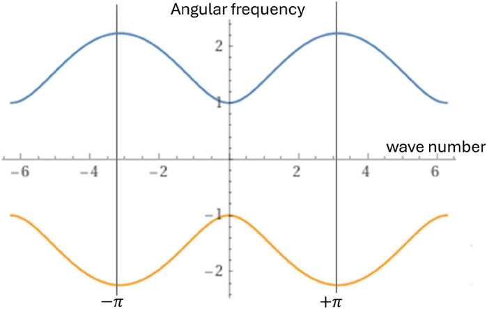
Figure 2. Schematic illustration of the discrete system dispersion relation $\omega \left(k\right)=\pm \sqrt{{\left({\alpha }^{\prime }\right)}^2+4{\beta }^2{\left(\sin \frac{ka}{2}\right)}^2}$ for $=1,$ $\beta =1$, and $\alpha =1$.

3.2 Eigenvectors

We now solve Equation 8 for the components of the amplitude vector $a_1$, $a_2$, $a_3$, and $a_4$, satisfying the dispersion relations given by Equation 11. Let us redefine $ka=2\theta$ such that $\left(e^{ika}-1\right)=e^{i\theta }\left(e^{i\theta }-e^{-i\theta }\right)$, $\left(1-e^{-ika}\right)=e^{-i\theta }\left(e^{i\theta }-e^{-i\theta }\right)$, and $\left(e^{ika}-1\right)\left(1-e^{-ika}\right)={\left(e^{i\theta }-e^{-i\theta }\right)}^2$. For the sake of simplifying the notation, we also define $X=\left(e^{i\theta }-e^{-i\theta }\right)$. With this notation, Equation 8 becomes the system of four linear equations:

$-i{\alpha }^{\prime }{a}_1+i\omega a_3+\beta e^{i\theta }X{a}_4=0(\mathrm{12a})$

$-i{\alpha }^{\prime }{a}_2+\beta e^{-i\theta }X{a}_3+i\omega a_4=0(\mathrm{12b})$

$i\omega a_1-\beta e^{i\theta }X{a}_2-i{\alpha }^{\prime }{a}_3=0(\mathrm{12c})$

$-\beta e^{-i\theta }X{a}_1+i\omega a_2-i{\alpha }^{\prime }{a}_4=0(\mathrm{12d})$

To find solutions to the system of equations given by Equations 12 a–d, we hypothesize that

$a_1=i{a}_4{e}^{i\theta }(\mathrm{13a})$

$a_2=-i{a}_3{e}^{-i\theta }(\mathrm{13b})$

$a_3=i\omega e^{i\frac{\theta }{2}}(\mathrm{13c})$

$a_4=e^{-i\frac{\theta }{2}}\left({\alpha }^{\prime }-\beta X\right)(\mathrm{13d})$

Recognizing that $\omega =\pm \sqrt{\left({\alpha }^{\prime }+\beta X\right)}\sqrt{\left({\alpha }^{\prime }-\beta X\right)}$, $\left({\alpha }^{\prime }-\beta X\right)=\sqrt{\left({\alpha }^{\prime }-\beta X\right)}\sqrt{\left({\alpha }^{\prime }-\beta X\right)}$, and $\left({\alpha }^{\prime }+\beta X\right)=\sqrt{\left({\alpha }^{\prime }+\beta X\right)}\sqrt{\left({\alpha }^{\prime }+\beta X\right)}$, the normalized amplitude eigenvector is obtained in the form

${\widehat{\zeta }}_k=\frac{1}{2\sqrt{\sqrt{{\left({\alpha }^{\prime }\right)}^2-{\beta }^2{X}^2}}}\left(\begin{array}{c}i{e}^{i\frac{\theta }{2}}\sqrt{{\alpha }^{\prime }-\beta X}\\ \pm e^{-i\frac{\theta }{2}}\sqrt{{\alpha }^{\prime }+\beta X}\\ \pm i{e}^{i\frac{\theta }{2}}\sqrt{{\alpha }^{\prime }+\beta X}\\ e^{-i\frac{\theta }{2}}\sqrt{{\alpha }^{\prime }-\beta X}\end{array}\right)(14)$

4 Evanescent waves

In order to find non-propagative solutions of the Dirac equations (Equation 5), we consider the ansatz

${\psi }_n={\xi }_{k^{\prime }}{e}^{i\omega t}{e}^{i\left(k+i{k}^{\prime }\right)na}=\left(\begin{array}{c}{b}_1\\ b_2\\ b_3\\ b_4\end{array}\right)e^{i\omega t}{e}^{i\left(k+i{k}^{\prime }\right)na}(15)$

We follow the procedure used in Section 3 to find the dispersion relation for waves of the form given by Equation 15:

$\omega =\pm \sqrt{{\left({\alpha }^{\prime }\right)}^2-{4\beta }^2{\left(\sinh \frac{k^{\prime }a}{2}\right)}^2}(16)$

When $k^{\prime }=0$, then $\omega ={\alpha }^{\prime }$, and $\omega =0$ when ${\left({\alpha }^{\prime }\right)}^2-{4\beta }^2{\left(\sinh \frac{k^{\prime }a}{2}\right)}^2$ = 0; that is, $\sinh \frac{k^{\prime }a}{2}=\pm \frac{\alpha }{2\beta }$ or equivalently $k^{\prime }=\frac{2}{a}{\sinh }^{-1}\left(\pm \frac{\alpha }{2\beta }\right)$. We denote this value of $k^{\prime }$ by ${k_0}^{\prime }$. The points $\pm k_0^{\prime }$ are illustrated schematically in Figure 3.

Figure 3

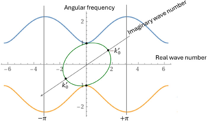
Figure 3. Schematic illustration of the discrete system dispersion relation for propagative waves (blue and yellow lines): $\omega \left(k\right)=\pm \sqrt{{{\alpha }^{\prime }}^2+4{\beta }^2{\left(\sin \frac{ka}{2}\right)}^2}$ for a $=1,$ $\beta =1$, and $\alpha =1$ and evanescent waves (green line) at $k=0$: $\omega \left(k^{\prime }\right)=\pm \sqrt{{{\alpha }^{\prime }}^2-{4\beta }^2{\left(\sinh \frac{k^{\prime }a}{2}\right)}^2}$.

The normalized amplitude eigenvector is of the form

${\widehat{\xi }}_{k^{\prime }}=\frac{1}{\sqrt{2{\alpha }^{\prime }\left(e^{{\theta }^{\prime }}+e^{-{\theta }^{\prime }}\right)}}\left(\begin{array}{c}i{e}^{-\frac{{\theta }^{\prime }}{2}}\sqrt{{\alpha }^{\prime }-\beta X^{\prime }}\\ \pm e^{\frac{{\theta }^{\prime }}{2}}\sqrt{{\alpha }^{\prime }+\beta X^{\prime }}\\ \pm i{e}^{-\frac{{\theta }^{\prime }}{2}}\sqrt{{\alpha }^{\prime }+\beta X^{\prime }}\\ e^{\frac{{\theta }^{\prime }}{2}}\sqrt{{\alpha }^{\prime }-\beta X^{\prime }}\end{array}\right)(17)$

—where $X^{\prime }=\left(e^{{-\theta }^{\prime }}-e^{{\theta }^{\prime }}\right)$ with $k^{\prime }a=2{\theta }^{\prime }$.

5 Berry phase for propagative waves

5.1 Continuous contribution to the Berry phase

The contribution of the continuous part of the function, ${\widehat{\zeta }}_k$ to the Berry connection (Berry, 1984) is given by

$BC\left(k\right)=-i{\widehat{\zeta }}_k^{*T}\frac{{\partial \widehat{\zeta }}_k}{\partial k}(18)$

Note that $\frac{{\partial \widehat{\zeta }}_k}{\partial k}=\frac{{\partial \widehat{\zeta }}_k}{\partial \theta }\frac{\partial \theta }{\partial k}=\frac{a}{2}\frac{{\partial \widehat{\zeta }}_k}{\partial \theta }$ since $ka=2\theta$, and therefore, Equation 18 gives us $BC\left(k\right)=0$ for all $k\in \left[-\frac{\pi }{a},\frac{\pi }{a}\right]$ for which ${\widehat{\zeta }}_k$ is continuous. So, the continuous contribution to the Berry connection is zero.

5.2 Contribution of discontinuities in the eigenvectors to the Berry connection

The eigenvector given by Equation 14 contains components in the form of square roots—$\sqrt{{\alpha }^{\prime }+\beta X}$ and $\sqrt{{\alpha }^{\prime }-\beta X}$—which are square roots of complex numbers.

The square root of a complex number is given by the formula

$\sqrt{A+iB}=\pm \left(\sqrt{\frac{A}{2}+\frac{1}{2}\sqrt{A^2+B^2}}+i\frac{B}{\left|B\right|}\sqrt{\frac{1}{2}\sqrt{A^2+B^2}-\frac{A}{2}}\right)$

Here, $A={\alpha }^{\prime }$ and $B=2\beta \sin \theta$. Near the origin on both sides (positive and negative) of the Brillouin zone: ${\theta }^{\pm }=0^{\pm }$, so $B\sim 2{\theta }^{\pm }=0^{\pm }$. We therefore have $\sqrt{{\alpha }^{\prime }+\beta X}\sim \pm (\sqrt{\frac{A}{2}+\frac{1}{2}\sqrt{A^2}}+i\frac{B}{\left|B\right|}\sqrt{\frac{1}{2}\sqrt{A^2}-\frac{A}{2}})=\left(\sqrt{\frac{A}{2}+\frac{1}{2}\left|A\right|}+i\frac{B}{\left|B\right|}\sqrt{\frac{1}{2}\left|A\right|-\frac{A}{2}}\right)$.

The phase of $\sqrt{A+iB}$ in the vicinity of the origin of the first Brillouin zone satisfies $\tan \phi \cong sgn\left(B\right)\frac{\sqrt{-A+\left|A\right|}}{\sqrt{A+\left|A\right|}}$.

If $A=+\alpha$—that is $A>0$—then $\left|A\right|=A$ and $\tan \phi \cong sgn\left(B\right)\frac{\sqrt{-A+A}}{\sqrt{A+A}}=0.$ The quantity $\sqrt{{\alpha }^{\prime }+\beta X}$ remains continuous at the origin of the Brillouin zone; the same is true for the quantity $\sqrt{{\alpha }^{\prime }-\beta X}.$ Therefore, in this case, there is no discontinuity in the complex amplitude, which leads to the Berry phase being equal to zero, as discussed in in Section 5.1.

If $A=-\alpha$, then $A<0$—that is, $\left|A\right|=-A$ and $\tan \phi \cong sgn\left(B\right)\frac{\sqrt{A+A}}{\sqrt{A-A}}=sgn\left(B\right)\infty .$ On the positive side of the origin of the Brillouin zone $B=0^{+}$, $sgn\left(B\right)>0$ and $\phi =\frac{\pi }{2}$. On the negative side of the origin of the Brillouin zone $B=0^{-}$, $sgn\left(B\right)<0$ and $\phi =-\frac{\pi }{2}$. The quantity $\sqrt{{\alpha }^{\prime }+\beta X}$ undergoes a π phase discontinuity at the origin of the Brillouin zone.

Considering the component $\sqrt{{\alpha }^{\prime }-\beta X}$, we still have $A={\alpha }^{\prime }$ but $B=-2\beta \sin \theta$. We still have a discontinuity when $A=-\alpha$, but then $\tan \phi \cong -sgn\left(B\right)\infty .$ On the positive side of the origin of the Brillouin zone $B=0^{-}$, $sgn\left(B\right)<0$ and $\phi =-\frac{\pi }{2}$. On the negative side of the origin of the Brillouin zone $B=0^{+}$, $sgn\left(B\right)>0$ and $\phi =+\frac{\pi }{2}$. The quantity $\sqrt{{\alpha }^{\prime }-\beta X}$ undergoes a -π phase discontinuity at the origin of the Brillouin zone.

In the case of $A<0,$ to calculate the discontinuity contribution of the components at $2\theta =ka=0$ to the Berry phase, consider two amplitude vectors on both sides of the origin of the Brillouin zone:

${\widehat{\zeta }}_{k\sim 0^{+}}\cong \frac{1}{2}\left(\begin{array}{c}i{e}^{-i\phi \left({\theta }^{+}\right)}\\ \pm e^{i\phi \left({\theta }^{+}\right)}\\ \pm {ie}^{i\phi \left({\theta }^{+}\right)}\\ e^{-i\phi \left({\theta }^{+}\right)}\end{array}\right)\text{\hspace{0.17em}and\hspace{0.17em}}{\widehat{\zeta }}_{k\sim 0^{-}}\cong \frac{1}{2}\left(\begin{array}{c}i{e}^{-i\phi \left({\theta }^{-}\right)}\\ \pm e^{i\phi \left({\theta }^{-}\right)}\\ \pm i{e}^{i\phi \left({\theta }^{-}\right)}\\ e^{-i\phi \left({\theta }^{-}\right)}\end{array}\right)$

Their inner product gives ${\widehat{\zeta }}_{k\sim 0^{+}}^{\mathrm{*T}}{\widehat{\zeta }}_{k\sim 0^{-}}\cong \cos \pi .$ Therefore, the change in geometric phase as the amplitude vector is crossing the origin of the first Brillouin zone is $\Delta \eta =\pi$. Now, the Berry phase is therefore the sum of the contributions from the continuous and the discontinuous parts of the amplitude vector, so the Berry phase is equal to $\pi$. Note that this phase is independent of the specific value of $\alpha$ as long as we consider the Dirac-factored equation with $-\alpha$.

The Berry phase is a topological invariant of the system. Dirac-factored equations $\left[\mathit{C}\frac{\partial }{\partial t}+\beta \left\{\mathit{A}{∆}^{+}+\mathit{B}{∆}^{-}\right\}-i\left(\pm \alpha \right)\mathit{I}\right]{\psi }_n=0$ describe two types of acoustic waves: one with a conventional topology (Berry phase equal to 0) and the other one with an unconventional topology (Berry phase of π). In the latter case, the acoustic waves are isomorphic to the quantum spin of an electron, which requires a closed path, corresponding to two Brillouin zones to recover the original eigen amplitude vector. This is an example of an acoustic pseudospin.

6 Berry phase for evanescent waves

We now compute the Berry connection of the unit amplitude vector ${\widehat{\xi }}_{k^{\prime }}$ given by Equation 17 along the loop given by the dispersion relation of the evanescent waves with $k=0$. Since $\omega$ is a real number, we have the restriction $-\frac{\alpha }{2\beta }\le \sinh \frac{k^{\prime }a}{2}\le \frac{\alpha }{2\beta }$ , which is equivalent to $-\frac{\alpha }{\beta }\le X^{\prime }\le \frac{\alpha }{\beta }$ —that is, $0\le \alpha +\beta X^{\prime }$ and $0\le \alpha -\beta X^{\prime }.$

We first compute the Berry connection along the top and the bottom halves of the loop, when $\omega >0$ and $\omega <0.$

Case 1. ${\alpha }^{\prime }=\alpha$ with $\omega >0$ or $\omega <0$.

In this case, the unit amplitude vector is ${\widehat{\xi }}_{k^{\prime }}=\frac{1}{\sqrt{2\alpha \left(e^{{\theta }^{\prime }}+e^{-{\theta }^{\prime }}\right)}}\left(\begin{array}{c}i{e}^{-\frac{{\theta }^{\prime }}{2}}\sqrt{\alpha -\beta X^{\prime }}\\ \pm e^{\frac{{\theta }^{\prime }}{2}}\sqrt{\alpha +\beta X^{\prime }}\\ \pm i{e}^{-\frac{{\theta }^{\prime }}{2}}\sqrt{\alpha +\beta X^{\prime }}\\ e^{\frac{{\theta }^{\prime }}{2}}\sqrt{\alpha -\beta X^{\prime }}\end{array}\right)$. Note that the quantities inside the square root are non-negative because of the restriction on $k^{\prime }$, so the unit amplitude vector is a continuous function of $k^{\prime }.$ Therefore, the Berry connection is given by

$BC\left(k^{\prime }\right)=-i{\widehat{\xi }}_{k^{\prime }}^{\mathrm{*T}}\frac{\partial {\widehat{\xi }}_{k^{\prime }}}{\partial k^{\prime }}$

We note that $\frac{\partial {\widehat{\xi }}_{k^{\prime }}}{\partial k^{\prime }}=\frac{\partial {\widehat{\xi }}_{k^{\prime }}}{\partial {\theta }^{\prime }}\frac{\partial {\theta }^{\prime }}{\partial k^{\prime }}=\frac{a}{2}\frac{\partial {\widehat{\xi }}_{k^{\prime }}}{\partial {\theta }^{\prime }}$ since $\left(k^{\prime }a=2{\theta }^{\prime }\right)$, which leads to $BC\left(k^{\prime }\right)=0.$

Therefore, the Berry connection when $\alpha ={\alpha }^{\prime }$ is zero along the top and bottom halves of the loop.

Case 2. ${\alpha }^{\prime }=-\alpha$ with $\omega >0$ or $\omega <0$.

In this case, the unit amplitude vector is ${\widehat{\xi }}_{k^{\prime }}=\frac{-1}{\sqrt{2\alpha \left(e^{{\theta }^{\prime }}+e^{-{\theta }^{\prime }}\right)}}\left(\begin{array}{c}i{e}^{-\frac{{\theta }^{\prime }}{2}}\sqrt{\alpha +\beta X^{\prime }}\\ \pm e^{\frac{{\theta }^{\prime }}{2}}\sqrt{\alpha -\beta X^{\prime }}\\ \pm i{e}^{-\frac{{\theta }^{\prime }}{2}}\sqrt{\alpha -\beta X^{\prime }}\\ e^{\frac{{\theta }^{\prime }}{2}}\sqrt{\alpha +\beta X^{\prime }}\end{array}\right)$. Again, the quantities inside the square root are non-negative. The Berry connection is thus given by $-i{\widehat{\xi }}_{k^{\prime }}^{\mathrm{*T}}\frac{\partial {\widehat{\xi }}_{k^{\prime }}}{\partial k^{\prime }}.$ A similar calculation to that in case ${\alpha }^{\prime }=\alpha$ gives us $BC\left(k^{\prime }\right)=0$ along the top and bottom halves of the loop.

Case 3. The Berry connection near the points where the loop intersects the $x$-axis.

We wish to determine whether near $\pm {k_0}^{\prime }$, ${\widehat{\xi }}_{k^{\prime },{\omega }^{+}}$, the unit amplitude vector at $k^{\prime }$ with positive $\omega$, is parallel or anti-parallel to ${\widehat{\xi }}_{k^{\prime },{\omega }^{-}}$, the unit amplitude vector at $k^{\prime }$ with negative $\omega$. We calculate the dot product

${\widehat{\xi }}_{k^{\prime },{\omega }^{+}}^{*}·{\widehat{\xi }}_{k^{\prime },{\omega }^{-}}=\frac{2\beta }{{\alpha }^{\prime }}\sinh {\theta }^{\prime }.$

As $k^{\prime }\to k_0^{\prime }$, note that $\omega \to 0$. So in that limit, the dispersion relation given by Equation 16 gives us $\frac{2\beta }{\left|{\alpha }^{\prime }\right|}=\frac{1}{\left|\sinh {\theta }^{\prime }\right|}.$ Therefore, when ${\alpha }^{\prime }=\alpha ,$ we have ${\widehat{\xi }}_{k^{\prime },{\omega }^{+}}^{*}·{\widehat{\xi }}_{k^{\prime },{\omega }^{-}}=\frac{\sinh {\theta }^{\prime }}{\left|\sinh {\theta }^{\prime }\right|}$ as $k^{\prime }\to k_0^{\prime }.$ When ${\alpha }^{\prime }=-\alpha ,$ we have ${\widehat{\xi }}_{k^{\prime },{\omega }^{+}}^{*}·{\widehat{\xi }}_{k^{\prime },{\omega }^{-}}=\frac{\sinh {\theta }^{\prime }}{\left|\sinh {\theta }^{\prime }\right|}$ as $k^{\prime }\to k_0^{\prime }.$ So, when ${\alpha }^{\prime }=\alpha$, ${\widehat{\xi }}_{k^{\prime },{\omega }^{+}·}^{*}·{\widehat{\xi }}_{k^{\prime },{\omega }^{-}}\to \frac{\sinh {\theta }^{\prime }}{\left|\sinh {\theta }^{\prime }\right|}=1$ as $k^{\prime }\to k_0^{\prime }$. Therefore, ${\widehat{\xi }}_{k^{\prime },{\omega }^{+}}^{*}$ and ${\widehat{\xi }}_{k^{\prime },{\omega }^{-}}$ are parallel. When ${\alpha }^{\prime }=-\alpha$, ${\widehat{\xi }}_{k^{\prime },{\omega }^{+}}^{*}·{\widehat{\xi }}_{k^{\prime },{\omega }^{-}}\to -\frac{\sinh {\theta }^{\prime }}{\left|\sinh {\theta }^{\prime }\right|}=-1$ as $k^{\prime }\to k_0^{\prime }.$ So, ${\widehat{\xi }}_{k^{\prime },{\omega }^{+}}^{*}$ and ${\widehat{\xi }}_{k^{\prime },{\omega }^{-}}$ are anti-parallel.

Similarly, when $k^{\prime }\to -k_0^{\prime },$ if ${\alpha }^{\prime }=\alpha$, ${\widehat{\xi }}_{k^{\prime },{\omega }^{+}}^{*}$ and ${\widehat{\xi }}_{k^{\prime },{\omega }^{-}}$ are anti-parallel, and if ${\alpha }^{\prime }=-\alpha$, ${\widehat{\xi }}_{k^{\prime },{\omega }^{+}}^{*}$ and ${\widehat{\xi }}_{k^{\prime },{\omega }^{-}}$ are parallel.

Therefore, along the closed loop over the evanescent mode, the Berry phase amounts to $\pi$ for both ${\alpha }^{\prime }=\pm \alpha .$

7 Interface modes

We now consider a system composed of two semi-infinite chains described by the acoustic Dirac equation, but differing only in the value of the parameter ${\alpha }^{\prime }$. Such a system may be realized by considering the mass spring system in Figure 1 (which is governed by the Klein–Gordon equation) (Calderin et al., 2019) and by considering evanescent waves corresponding to the $+\alpha$ Dirac equation for masses with a negative label and $-\alpha$ Dirac equation for masses with a positive label (since solutions to the Dirac equations are solutions to the Klein–Gordon equation). The consideration of such waves is mathematical. Figure 4 describes the set up.

Figure 4

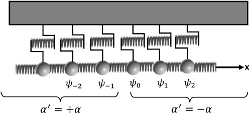
Figure 4. Schematic illustration of an interface between two topologically different semi-infinite media obeying the acoustic Dirac equation. The medium with ${\alpha }^{\prime }=-\alpha$ is topologically non-trivial, and the medium with ${\alpha }^{\prime }=+\alpha$ is topologically trivial.

At the interface, the Dirac equations are

$\left[\mathit{C}\frac{\partial }{\partial t}+\beta \left\{\mathit{A}{∆}^{+}+\mathit{B}{∆}^{-}\right\}-i\left(+\alpha \right)\mathit{I}\right]{\psi }_{n=-1}=0(\mathrm{19a})$

$\left[\mathit{C}\frac{\partial }{\partial t}+\beta \left\{\mathit{A}{∆}^{+}+\mathit{B}{∆}^{-}\right\}-i\left(-\alpha \right)\mathit{I}\right]{\psi }_{n=0}=0(\mathrm{19b})$

The Equations 19 a,b can be expanded as

$\left[\mathit{C}\frac{\partial }{\partial t}{\psi }_{-1}+\beta \left\{\mathit{A}\left({\psi }_0-{\psi }_{-1}\right)+\mathit{B}\left({\psi }_{-1}-{\psi }_{-2}\right)\right\}-i\left(+\alpha \right)\mathit{I}{\psi }_{-1}\right]=0(\mathrm{20a})$

$\left[\mathit{C}\frac{\partial }{\partial t}{\psi }_0+\beta \left\{\mathit{A}\left({\psi }_1-{\psi }_0\right)+\mathit{B}\left({\psi }_0-{\psi }_{-1}\right)\right\}-i\left(-\alpha \right)\mathit{I}{\psi }_0\right]=0(\mathrm{20b})$

We now seek solutions to these equations that take the form of evanescent waves decaying on both sides of the interface. These are solutions of the form

${\psi }_n={\left(\begin{array}{c}{b}_1\\ b_2\\ b_3\\ b_4\end{array}\right)}_{+\alpha ,k^{\prime }>0}{e}^{i\omega t}{e}^{k^{\prime }na}ifn<-1(\mathrm{21a})$

${\psi }_n={\left(\begin{array}{c}{b}_1\\ b_2\\ b_3\\ b_4\end{array}\right)}_{-\alpha ,-k^{\prime }<0}{e}^{i\omega t}{e}^{-k^{\prime }na}ifn>0.(\mathrm{21b})$

Equations 21 a,b give are solutions to the bulk acoustic Dirac equation of infinite chains, each with its respective values of ${\alpha }^{\prime }$. At the interface, we consider

${\psi }_{-1}={\left(\begin{array}{c}{W}_{-1}\\ X_{-1}\\ Y_{-1}\\ Z_{-1}\end{array}\right)}_{+\alpha ,k^{\prime }>0}{e}^{i\omega t}{e}^{-k^{\prime }a}(\mathrm{22a})$

${\psi }_0={\left(\begin{array}{c}{W}_0\\ X_0\\ Y_0\\ Z_0\end{array}\right)}_{-\alpha ,-k^{\prime }<0}{e}^{i\omega t}(\mathrm{22b})$

The existence of solutions in the forms given by Equations 22a,bwhich satisfy Equations 20a,b implies the existence of interface modes between the two chains with different topologies.

Inserting Equations 22a,b,b into Equations 20a,b,b gives us a system of eight linear equations in the eight unknowns $W_{-1}$, $X_{-1}$, $Y_{-1}$, $Z_{-1}$, $W_0$, $X_0$, $Y_0$, and $Z_0$:

$\left(\begin{array}{cccccccc}-i\left(+\alpha \right)& 0& i\omega & -\beta & 0& 0& 0& \beta e^{k^{\prime }a}\\ 0& -i\left(+\alpha \right)& \beta & i\omega & 0& 0& 0& 0\\ i\omega & \beta & -i\left(+\alpha \right)& 0& 0& {-\beta e}^{k^{\prime }a}& 0& 0\\ -\beta & i\omega & 0& -i\left(+\alpha \right)& 0& 0& 0& 0\\ 0& 0& 0& 0& -i\left(-\alpha \right)& 0& i\omega & -\beta \\ 0& 0& -\beta e^{-k^{\prime }a}& 0& 0& -i\left(-\alpha \right)& \beta & i\omega \\ 0& 0& 0& 0& i\omega & \beta & -i\left(-\alpha \right)& 0\\ \beta e^{-k^{\prime }a}& 0& 0& 0& -\beta & i\omega & 0& -i\left(-\alpha \right)\end{array}\right)\left(\begin{array}{c}\begin{array}{c}{W}_{-1}\\ X_{-1}\\ Y_{-1}\\ Z_{-1}\end{array}\\ \begin{array}{c}{W}_0\\ X_0\\ Y_0\\ Z_0\end{array}\end{array}\right)=\left(\begin{array}{c}0\\ {\beta b}_3^{+}{e}^{-k^{\prime }a}\\ 0\\ -\beta b_1^{+}{e}^{-k^{\prime }a}\\ -\beta b_4^{-}{e}^{-k^{\prime }a}\\ 0\\ \beta b_2^{-}{e}^{-k^{\prime }a}\\ 0\end{array}\right)(23)$

Equation 23 has solutions if the $8\times 8$ matrix is invertible—that is, if its determinant is not equal to zero. By defining $a=i\left(+\alpha \right)/\beta$, $b=i\omega /\beta$, and $c=1$, we calculate the determinant of that matrix to be

$\det \left(\omega \right)=b^8+b^6\left(-4a^2+6\right)+b^4\left(6a^4-14a^2+11\right)+b^2\left(-4a^6+10a^4-14a^2+6\right)+a^8-2a^6+3a^4-2a^2+1(24)$

Note that this determinant is independent of k’. To illustrate, let us set $\beta =\alpha =1$ and plot $\det \left(\omega \right)={\omega }^8-10{\omega }^6+31{\omega }^4-34{\omega }^2+9$ .

The $\det \left(\omega \right)$ is non-zero for the majority of frequencies corresponding to evanescent waves, except for the two frequencies $\omega =\pm \frac{1}{2}\left(\sqrt{5}-1\right)$ . There exist solutions to Equation 24 within this range of real frequencies. The interface between the chains with trivial and nontrivial topologies supports localized interfacial modes. These are topological interfacial modes. In Figure 5 there are two values of $\omega$ for which det( $\omega$ ) = 0. This implies that there are no real frequency solutions, although there may be solutions with complex frequencies. These waves may decay as a function of time.

Figure 5

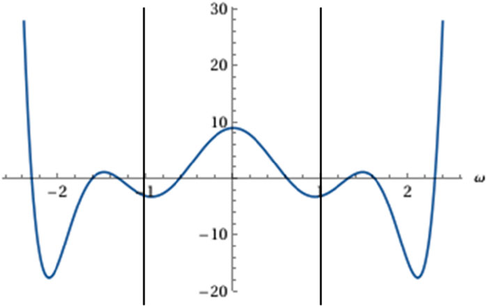
Figure 5. Plot of $\det \left(\omega \right)={\omega }^8-10{\omega }^6+31{\omega }^4-34{\omega }^2+9$ . The region between the vertical lines corresponds to the frequency range of evanescent waves for $\alpha =1$ .

8 Conclusion

We have here demonstrated that the Dirac factorization of the equations of motion of a mass and spring model exposes the potential for topological insulator behavior in acoustic systems. In particular, for a 1-d harmonic mass and spring chain attached elastically to a rigid substrate, the equations of motion give rise to a discrete version of the Klein–Gordon equation that can be factorized into Dirac equations with broken time-reversal and parity symmetry. Propagative and evanescent wave solutions of the Dirac factored equations were obtained. For propagative modes, the Berry phase for the Dirac equation with the + sign was found to be zero (conventional topology), and that with the – sign was found to be $\pi$ (non-conventional topology). In contrast, for the evanescent mode, the Berry phase was $\pi$ for both the + and – equations. Using the distinction between topologies for the propagative waves, we demonstrated the existence of a topologically protected interface mode between conventional and non-conventional topologies.

Dirac factorization of classical wave equations exposes the possibility of topological insulators arising from broken symmetries. It reveals the possibilities offered by symmetry breaking in terms of the direction of wave propagation. However, additional physical conditions or mechanisms are needed to break T- or P-symmetry and realize one-way propagating waves in physical systems.

Data availability statement

The original contributions presented in the study are included in the article/supplementary material; further inquiries can be directed to the corresponding author.

Author contributions

AB: Writing – original draft, Writing – review and editing. KR: Writing – original draft, Writing – review and editing. PD: Writing – original draft, Writing – review and editing.

Funding

The author(s) declare that financial support was received for the research and/or publication of this article. This work was supported by the Science and Technology Center New Frontiers of Sound (NewFoS) through NSF cooperative agreement # 2242925.

Conflict of interest

The authors declare that the research was conducted in the absence of any commercial or financial relationships that could be construed as a potential conflict of interest.

Generative AI statement

The author(s) declare that no Generative AI was used in the creation of this manuscript.

Any alternative text (alt text) provided alongside figures in this article has been generated by Frontiers with the support of artificial intelligence and reasonable efforts have been made to ensure accuracy, including review by the authors wherever possible. If you identify any issues, please contact us.

Publisher’s note

All claims expressed in this article are solely those of the authors and do not necessarily represent those of their affiliated organizations, or those of the publisher, the editors and the reviewers. Any product that may be evaluated in this article, or claim that may be made by its manufacturer, is not guaranteed or endorsed by the publisher.

References

Berry, M. V. (1984). Quantal phase factors accompanying adiabatic changes. Proc. R. Soc. Lond. A39245–57. doi:10.1098/rspa.1984.0023

CrossRef Full Text | Google Scholar

Calderin, L., Hasan, M. A., Jenkins, N. G., Lata, T., Lucas, P., Runge, K., et al. (2019). Experimental demonstration of coherent superpositions in an ultrasonic pseudospin. Sci. Rep. 9, 14156. doi:10.1038/s41598-019-50366-y

PubMed Abstract | CrossRef Full Text | Google Scholar

Chang, C.-Z., Liu, C.-X., and MacDonald, A. H. (2023). Colloquium: Quantum anomalous hall effect. Rev. Mod. Phys. 95 (1), 011002. doi:10.1103/RevModPhys.95.011002

CrossRef Full Text | Google Scholar

Chen, Z., He, H., Li, H., Li, M., Kou, J., Lu, Y., et al. (2024). Observation of parity-time symmetry for evanescent waves. Commun. Phys. 7, 339. doi:10.1038/s42005-024-01816-1

CrossRef Full Text | Google Scholar

Deng, Y., Ge, H., Tian, Y., Lu, M., and Jing, Y. (2017). Observation of zone folding induced acoustic topological insulators and the role of spin-mixing defects. Phys. Rev. B 96, 184305. doi:10.1103/PhysRevB.96.184305

CrossRef Full Text | Google Scholar

Deymier, P., and Runge, K. (2016). One-dimensional mass-spring chains supporting elastic waves with non-conventional topology. Crystals 6 (4), 44. doi:10.3390/cryst6040044

CrossRef Full Text | Google Scholar

Deymier, P. A., and Runge, K. (2022). Revealing topological attributes of stiff plates by dirac factorization of their 2D elastic wave equation. Appl. Phys. Lett. 120 (8), 081701. doi:10.1063/5.0086559

CrossRef Full Text | Google Scholar

Deymier, P. A., Runge, K., Swinteck, N., and Muralidharan, K. (2014). Rotational modes in a phononic crystal with fermion-like behavior. J. Appl. Phys. 115, 163510. doi:10.1063/1.4872142

CrossRef Full Text | Google Scholar

Deymier, P. A., Runge, K., Swinteck, N., and Muralidharan, K. (2015). Torsional topology and fermion-like behavior of elastic waves in phononic structures. Comptes Rendus Mécanique 343, 700–711. doi:10.1016/j.crme.2015.07.003

CrossRef Full Text | Google Scholar

Hasan, M. Z., and Kane, C. L. (2010). Colloquium: topological insulators. Rev. Mod. Phys. 82 (4), 3045–3067. doi:10.1103/RevModPhys.82.3045

CrossRef Full Text | Google Scholar

He, C., Ni, X., Ge, H., Sun, X.-C., Chen, Y.-B., Lu, M.-H., et al. (2016). Acoustic topological insulator and robust one-way sound transport. Nat. Phys. 12, 1124–1129. doi:10.1038/nphys3867

CrossRef Full Text | Google Scholar

Kane, C. L., and Lubensky, T. C. (2014). Topological boundary modes in isostatic lattices. Nat. Phys. 10, 39–45. doi:10.1038/nphys2835

CrossRef Full Text | Google Scholar

Khanikaev, A. B., Fleury, R., Mousavi, S. H., and Alù, A. (2015). Topologically robust sound propagation in an angular-momentum-biased graphene-like resonator lattice. Nat. Commun. 6, 8260. doi:10.1038/ncomms9260

PubMed Abstract | CrossRef Full Text | Google Scholar

Mei, J., Chen, Z., and Wu, Y. (2016). Pseudo-time-reversal symmetry and topological edge states in two-dimensional acoustic crystals. Sci. Rep. 6, 32752. doi:10.1038/srep32752

PubMed Abstract | CrossRef Full Text | Google Scholar

Ni, X., He, C., Sun, X.-C., Liu, X.-p., Lu, M.-H., Feng, L., et al. (2015). Topologically protected one-way edge mode in networks of acoustic resonators with circulating air flow. New J. Phys. 17, 053016. doi:10.1088/1367-2630/17/5/053016

CrossRef Full Text | Google Scholar

Qi, X.-L., and Zhang, S.-C. (2010). The quantum spin hall effect and topological insulators. Phys. Today 63 (1), 33–38. doi:10.1063/1.3293411

CrossRef Full Text | Google Scholar

Qi, X.-L., and Zhang, S.-C. (2011). Topological insulators and superconductors. Rev. Mod. Phys. 83 (4), 1057–1110. doi:10.1103/RevModPhys.83.1057

CrossRef Full Text | Google Scholar

Qi, X.-L., Wu, Y.-S., and Zhang, S.-C. (2006). Topological quantization of the spin hall effect in two-dimensional paramagnetic semiconductors. Phys. Rev. B 74, 085308. doi:10.1103/PhysRevB.74.085308

CrossRef Full Text | Google Scholar

Süsstrunk, R., and Huber, S. D. (2016). Classification of topological phonons in linear mechanical metamaterials. Proc. Natl. Acad. Sci. U.S.A. 113 (33), E4767–E4775. doi:10.1073/pnas.1605462113

PubMed Abstract | CrossRef Full Text | Google Scholar

Xia, B.-Z., Liu, T.-T., Huang, G.-L., Dai, H.-Q., Jiao, J.-R., Zang, X.-G., et al. (2017). Topological phononic insulator with robust pseudospin-dependent transport. Phys. Rev. B 96, 094106. doi:10.1103/PhysRevB.96.094106

CrossRef Full Text | Google Scholar

Xue, H., Yang, Y., and Zhang, B. (2022). Topological acoustics. Nat. Rev. Mater 7, 974–990. doi:10.1038/s41578-022-00465-6

CrossRef Full Text | Google Scholar

Yang, Z., Gao, F., Shi, X., Lin, X., Gao, Z., Chong, Y., et al. (2015). Topological acoustics. Phys. Rev. Lett. 114, 114301. doi:10.1103/PhysRevLett.114.114301

PubMed Abstract | CrossRef Full Text | Google Scholar

Yves, S., Fleury, R., Lemoult, F., Fink, M., and Lerosey, G. (2017). Topological acoustic polaritons: robust sound manipulation at the subwavelength scale. New J. Phys. 19, 075003. doi:10.1088/1367-2630/aa66f8

CrossRef Full Text | Google Scholar

Zhang, Z., Wei, Q., Cheng, Y., Zhang, T., Wu, D., and Liu, X. (2017). Topological creation of Acoustic pseudospin multipoles in a flow-free symmetry-broken metamaterial lattice. Phys. Rev. Lett. 118, 084303. doi:10.1103/PhysRevLett.118.084303

PubMed Abstract | CrossRef Full Text | Google Scholar