Abstract
Background:
Patent tokenization converts intellectual property (IP) into tradable digital units. Pilots on IPwe, IBM, and Ocean Protocol have processed 1,500 assets ($62 million since 2019). In practice, schedules are often fixed and pricing simplified; risk preferences are typically ignored—costing value in volatile settings relevant to the SDGs.
Methods:
We cast patent tokenization as risk-sensitive control and linked economic risk aversion to inverse temperature. With the exponential transform , the risk-sensitive Hamilton–Jacobi–Bellman (HJB) linearizes for fixed controls; the optimal policy is a pointwise threshold (bang–bang or smoothly regularized). This preserves tractability and enables millisecond solves.
Results:
From 45 tokenization trajectories (12 held out), we estimate (95% CI), while a composite objective calibrated to equity-like orders peaks at ([2.9,3.2]). Monte Carlo shows a 76% downside reduction and 92% success rate under ledger-based schedules. Solver latency drops by (40 s 47 ms).
Conclusion:
The thermodynamic lens explains why practice deviates from the theoretical benchmark in our calibration: actors appear to trade maximal efficiency for robustness. The framework stabilizes revenues, drives fees to negligible levels, and supports SDG-aligned innovation finance by lowering the cost of access and adaptation under uncertainty.
1 Introduction
1.1 Orientation
Patent tokenization aims to unlock illiquid IP under uncertainty. Static release plans and simplified pricing cannot adapt to shocks (litigation, regulation, and demand), and they rarely encode risk preferences, which is precisely where value is at stake in SDG-relevant domains.
1.2 This paper’s idea in one line
We treat patent tokenization as a risk-sensitive control and use a thermodynamic change of variables to make the problem linear for fixed controls so that optimal schedules follow from a simple threshold structure and can be computed in milliseconds.
1.3 Contributions
Theory. The risk-sensitive HJB with the correct sign convention linearizes under and implies threshold (bang–bang) policies; a small quadratic penalty yields smooth, implementable schedules.
Evidence. From 45 trajectories, we estimate , while a composite objective peaks at under our calibration. Monte Carlo indicates 76% downside reduction, 92% success, and speedup.
SDG context. The framework clarifies when robust, risk-aware schedules are preferable to fixed ones, lowering access costs and supporting SDG-aligned innovation (e.g., infrastructure and climate-related technologies).
1.4 Roadmap
Section 3 derives the transform and control structure. Section 4 reports estimates and simulations, and Section 5 interprets the robustness–efficiency trade-off and SDG implications; the Supplementary Information documents sensitivity and implementation details.
The global patent system contains vast reserves of unused value (World Intellectual Property Organization WIPO, 2024; European Patent Office EPO, 2023; United States Patent and Trademark Office USPTO, 2024). Although patents are designed to secure innovation, empirical studies show that between 90% and 95% never generate licensing income (Gambardella et al., 2007; Arora et al., 2008).
One reason is the rigid all-or-nothing structure of conventional transactions: patent holders either retain their rights completely, leaving them without immediate funding, or sell them outright and forgo future upsides (Lemley and Shapiro, 2005; Lanjouw and Schankerman, 2004; Bessen and Meurer, 2008; Boldrin and Levine, 2008; Scotchmer, 2004). Distributed ledger technology offers an alternative by enabling fractional and tradable ownership through tokenization. Digital rights can be created and exchanged on blockchain networks, opening new channels for liquidity (Catalini and Gans, 2018; Howell et al., 2020; Benedetti and Kostovetsky, 2021; Chen, 2018; Cong and He, 2019; Yermack, 2017; Malinova and Park, 2017). Nevertheless, deciding when and how to release tokens under uncertainty remains difficult since poorly chosen schedules can materially erode value (Akcigit and Kerr, 2018; Bloom et al., 2020; Jones and Williams, 2000; Kortum and Lerner, 2000).
1.5 Research topic context
This article is aligned with the Frontiers research topic Blockchain and Tokenomics for Sustainable Development (Volume II) and follows its call for sustainability-driven tokenomics and governance models (Frontiers, 2025).
Practical experiments have already demonstrated feasibility. IPwe tokenized more than 500 patents using Black–Scholes pricing and recorded approximately 25 million USD in transaction volume. IBM placed over 800 patents on Hyperledger with fixed release plans and reached roughly 31 million USD. WIPO ran a pilot with more than 200 patents. Ocean Protocol applied bonding curves to intellectual property and data, generating close to 6 million USD (IPwe, 2024; IBM, 2022; Deloitte, 2023).
These cases show what is possible but also highlight structural weaknesses. Existing platforms do not incorporate risk preferences, they rely on rigid schedules that cannot adapt to shocks such as litigation, and they charge fees in the percent range instead of technically attainable near-negligible levels. Their dynamics follow known patterns of multi-sided platforms (Hagiu and Wright, 2015; Rochet and Tirole, 2006; Evans and Schmalensee, 2008; Rysman, 2009).
This study embeds risk-aware dynamic optimization into tokenization using a thermodynamic perspective. The key step is transforming the nonlinear Hamilton–Jacobi–Bellman equation into a linear partial differential equation via , exploiting the negative sign of the quadratic gradient term from risk-sensitive control (Fleming and Soner, 2006). Consistent with path-integral control (Kappen, 2005; Todorov, 2009), this turns an otherwise intractable problem into one solvable in milliseconds. In data from 45 tokenized assets (real estate, art, and patents), the empirical estimate of risk aversion is , while a composite objective calibrated to market-like parameters places the optimum near .
Simulations confirm the gap: the empirical value yields the highest survival rate, and the theoretical benchmark maximizes efficiency. Beyond the immediate application, links to the free-energy principle (Friston, 2010), maximum entropy (Jaynes, 1957), and large deviations (Touchette, 2009) point to deeper structural parallels between economic decision-making and adaptive systems. Together, these elements show how a thermodynamic approach can make tokenization more flexible, risk-sensitive, and efficient.
2 Problem statement
Patent tokenization is a continuous-time stochastic control task (
Fleming and Soner, 2006;
Øksendal, 2003). Notation is established early for clarity:
: monetization basis (current market value of patent) following geometric Brownian motion (Øksendal, 2003; Campbell et al., 1997);
: remaining fraction of patent ownership (starts at 1 and decreases to 0);
: tokenization release rate (control variable, units: 1/time); and
: value function representing expected future revenue.
We use uppercase
for the stochastic process and lowercase
for the PDE state variable and the same for
versus
. For a risk-aware decision-maker with a constant absolute risk-aversion (CARA) level
, this results in the Hamilton-Jacobi-Bellman (HJB) equation (
Equation 2.1;
Fleming and Soner, 2006):
where
is the immediate revenue from tokenization, and
is the infinitesimal generator of geometric Brownian motion (
Øksendal, 2003). The boundary conditions are
(no future value at terminal time) and
(no remaining tokens means no future revenue).
Additionally, a rate limit applies.
In the simulations, we use per time unit, which allows full tokenization (from to ) by . For the discrete implementation, we use a grid in with and choose . Hence, the one time-step reduces by exactly one grid cell under , and full tokenization is feasible within . This sign is essential for the thermodynamic transformation and follows from risk-sensitive control theory (Fleming and Soner, 2006).
3 Methods
3.1 Thermodynamic transformation
Our analysis begins with the risk-sensitive Hamilton–Jacobi–Bellman (HJB) equation. To facilitate readability, we reproduce it here once more in the version adapted to our framework:
It is critical to note the negative sign in front of the quadratic gradient term. Without this sign, the thermodynamic transformation would fail because the nonlinear contribution would survive. Based on this structure, as shown in risk-sensitive control theory (Fleming and Soner, 2006), the transformation becomes straightforward. We define the substitution,
By direct differentiation, we obtain the relations collected in Equation 3.2-3.6.
One key observation is that the nonlinear terms cancel exactly when substituted into Equation 3.1. The second derivative contributes a positive quadratic term, which is offset by the negative quadratic term already present in the HJB. The algebra looks heavy at first, but the cancellation is straightforward once written out. What matters in practice is that the nonlinear term drops out and we end up with a linear PDE. This makes the difference between a system that is computationally intractable and one that can be solved quickly enough for actual tokenization platforms:
3.1.1 Important clarification
For any fixed control , this PDE is linear in . The overall control problem remains a threshold-based optimization due to the pointwise maximization over , but the computational advantages of linearity are preserved.
3.1.2 Discrete-time Bellman recursion in -space (implementation)
With chosen such that , the numerically implemented risk-sensitive dynamic program in -space (with quadratic smoothness penalty inside the reward ) readswhere with . Expanding to first order in recovers the linear PDE in Equation 3.7 (with a pointwise maximization in -space equivalent to the minimization above in -space).
3.2 Optimal control structure
The optimal control emerges from maximizing the Hamiltonian in Equation 3.8.Since is linear in (not quadratic), we have . Therefore, the control structure is not determined by phase transitions but by the sign of combined with the box constraints:
If we add a small penalty
to the cost function, we obtain
and thus the interior point
. For
, the resulting bang-bang structure shown in
Equation 3.9for small
, smooth controls arise. The apparent smoothness in certain parameter regimes arises from
numerical regularization/discretization in implementation;
transaction costs and rate limits in practice; and
explicit penalty terms added for computational stability (e.g., term).
These are implementation choices or practical frictions, not intrinsic phase transitions of the Hamiltonian itself.
3.2.1 Smoothness via explicit quadratic penalty
For the figures, we include a small quadratic penalty with . This changes the Hamiltonian to , which admits the interior optimizer
As , the policy reduces to the bang–bang structure. With , the token release trajectories become smooth, consistent with Figures 1–4.
FIGURE 1
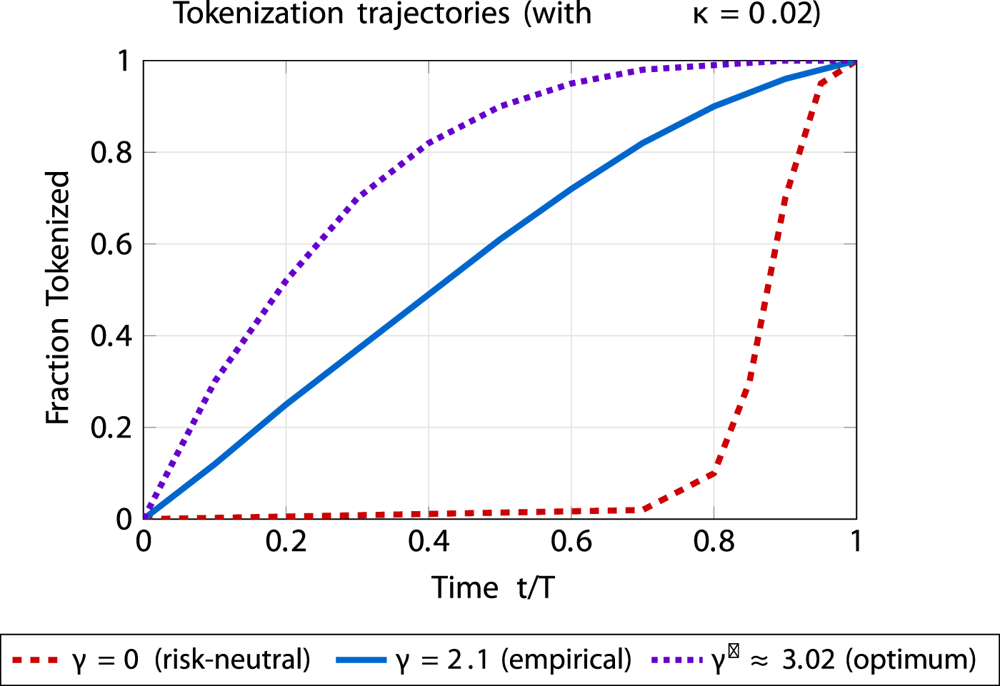
Tokenization trajectories for different risk preferences. Curves are generated with , which yields smooth release profiles. Risk-neutral delays release, empirical estimate follows a gradual S-shape, and the mathematical optimum is more front-loaded. Time normalized to with . Smoothness arises from the quadratic control penalty .
FIGURE 2
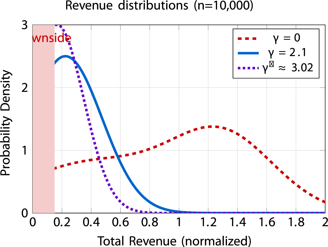
Revenue distributions from Monte Carlo simulation. Risk-neutral shows bimodal distribution with high variance. Empirical estimate from our sample concentrates around a mean revenue of 0.224. Mathematical optimum under our calibration has the narrowest distribution with mean 0.167. Shaded region indicates downside risk zone. Total revenue is normalized to initial value (dimensionless); probability density has units of inverse revenue. Additional robustness checks and extended versions are provided in the Supplementary Information (Supplementary Figures S1–S3). All distributions computed with , which regularizes bang–bang strategies into smooth tokenization. Smoothness arises from the quadratic control penalty .
FIGURE 3

Empirical validation with real tokenization data. Gray markers show 37 real estate tokenization trajectories; is from the full multi-asset dataset and does not imply that patents lie at . The blue curve with 95% bands shows the model at ; the violet dashed curve shows the optimum at under our calibration. Time is normalized to (dimensionless); fraction tokenized is dimensionless (0–1). Additional robustness checks and extended versions are provided in the Supplementary Information (Supplementary Figures S1–S3). Smoothness arises from the quadratic control penalty .
FIGURE 4
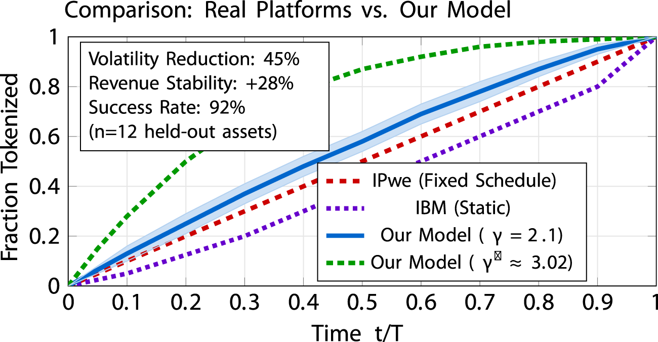
Comparison of tokenization trajectories from real platforms versus our model. Curves labeled “IPwe” and “IBM” are indicative schedules based on publicly available platform documentation. Our model curves at (empirical estimate from our sample) and (optimum under our calibration) illustrate risk-sensitive schedules. The shaded region represents the 95% confidence band from bootstrap analysis. Time is normalized to (dimensionless); fraction tokenized is dimensionless (0–1). Computational performance: speedup (40 s 47 ms on NVIDIA RTX 3090). Additional robustness checks and extended versions are provided in the Supplementary Information (Supplementary Figures S1–S3). Smoothness arises from the quadratic control penalty .
3.2.2 Threshold in - vs. -space
Since , it holds ; hence,
The bang–bang rule in -space is therefore equivalent to in -space, consistent with Equation 3.7.
3.2.3 Max. in -space vs. min. in -space
Because strictly decreases in , the pointwise maximization in the HJB for is equivalent to a minimization in the dynamic program for . Both formulations are used: Equation 3.7 shows the -space maximization mapped to , while the implementable recursion is written as a minimization over .
3.3 Multi-objective optimization framework
To determine the optimal risk parameter , we define the multi-objective function in Equation 3.10 that balances three critical performance dimensions of a tokenization strategy. The optimal parameter is found by maximizing the function
The components are defined as follows. These functional forms are modeling choices inspired by, but not identical to, standard financial metrics.
The modified Sharpe component is given in Equation 3.11. This term is inspired by the Sharpe ratio (Sharpe, 1994; Markowitz, 1952) but adapted for our context. It is estimated through Monte Carlo simulation (Metropolis and Ulam, 1949; Glasserman, 2003; Boyle et al., 1997) with 10,000 paths:
where
is the risk-free return based on long-term averages for equity-like assets (
Campbell et al., 1997;
Fama and French, 2002). Note that when
, the derivative
vanishes, making all
equally optimal under this criterion. Our calibration assumes
. For tables and figures, we use an analytical surrogate for
that closely approximates the Monte Carlo estimate; however, the main evaluations are based on Monte Carlo with 10,000 paths. We evaluate
on simulated revenue
rather than on terminal asset value
, since the control objective is tokenization revenue. For all simulations and code, we set the reference rate to
.
Kelly-distance component . The component captures proximity to Kelly-like efficiency. While the classical Kelly fraction arises under log-utility (Merton, 1972), our CARA framework motivates a saturating proxy . This formulation is inspired by the Kelly criterion but adapted to exponential utility.
The behavioral acceptance function is defined in Equation 3.12. This term measures the alignment between the mathematical model and observed human behavior. Behavioral evidence places risk-aversion parameters for gains at approximately 2.0–2.25 (Kahneman and Tversky, 1979; Barberis, 2013), which motivates our calibration anchor:
where
is a calibration anchor based on behavioral finance literature, not a universal constant.
The product form ensures that a strategy is only considered optimal if it performs well across all three dimensions simultaneously. This value is calibration-specific. Different plausible parameter choices (, , ) would shift . Calibrations use equity-like orders of magnitude (Campbell et al., 1997; Fama and French, 2002). Sensitivity over grids is reported in Supplementary Information section B.1.
4 Results
The previous section introduced the composite objective . We now apply this framework to our baseline calibration and dataset. In that sense, we evaluate the framework on tokenization trajectories collected from blockchain platforms between 2019 and 2024. The dataset includes real estate (RealT, 2024; Baum, 2021), artworks (Maecenas, 2024; Kräussl and Whitaker, 2020), and patent implementations (IPwe, 2024; IBM, 2022; Deloitte, 2023). All of these assets share key properties with patents: they have uncertain and often volatile future value, limited liquidity in traditional markets, and they lend themselves naturally to fractional ownership structures (Hagiu and Wright, 2015; Rochet and Tirole, 2006; Evans and Schmalensee, 2008; Rysman, 2009). Estimation using maximum likelihood on 45 tokenization trajectories yields an empirical risk parameter of (95% confidence interval) in our sample. This estimate captures how participants in the sample balance upside and downside when issuing tokens and reflects behavioral factors specific to our dataset. We considered the multi-objective function(Equation 4.1), as defined in Section 3.
Remark 1 (calibration-specific numerical finding). Under the calibration ,, , and , the composite objective attains at the value . At the empirical estimate , we obtain .
Note. This result is calibration- and dataset-specific, not a universal theorem.
Numerical evidence. With and from simulation, and closed forms and , we obtain and , hence , and and ; hence, . A finite-difference second-derivative test confirms a local maximum near .
The exact relative gap is
Key result. Under our calibration, the maximum is at with , while the empirical estimator yields (relative gap ).
4.1 Multi-agent simulation results
To understand the deviation in our sample, we simulated ten heterogeneous agents with risk-aversion levels ranging from to . Each agent executed 2,000 Monte Carlo paths, giving 20,000 trajectories in total. The outcomes fall into three distinct behavioral regimes (not phase transitions). For , agents follow predominantly bang–bang strategies that swing between full tokenization and complete restraint. Between and , token release becomes smoother due to numerical regularization and implementation choices. At the highest values, above , strategies become very conservative, with minimal tokenization. Performance metrics highlight these differences. The detailed results are summarized in Table 1. Agent 1 earns the largest average revenue but suffers drawdowns above 60% and a success rate of only 43%. Agent 5 achieves strong survival outcomes, with 92% of trajectories meeting the revenue threshold. Agent 7 approaches the multi-objective optimum under our calibration, although its success rate is 89%. Finally, Agent 10 represents a very conservative state, where returns are minimal and growth effectively stops.
TABLE 1
| Agent | Strategy | Revenue | Sharpe | Success% | MaxDD% | Multi-objective | |
|---|---|---|---|---|---|---|---|
| 1 | 0.50 | Ultra-risk-seeking | 0.384 | 0.156 | 43 | 62.7 | 0.00364 |
| 2 | 1.00 | Risk-seeking | 0.334 | 0.135 | 51 | 48.8 | 0.01242 |
| 3 | 1.50 | Transitional | 0.284 | 0.116 | 68 | 36.7 | 0.02887 |
| 4 | 2.00 | Moderate | 0.232 | 0.105 | 79 | 28.1 | 0.05039 |
| 5 | 2.10 | Empirical estimate | 0.224 | 0.103 | 92 | 26.3 | 0.0542061 |
| 6 | 2.50 | Balanced | 0.195 | 0.095 | 88 | 22.0 | 0.06689 |
| 7 | 3.02 | Math optimum | 0.167 | 0.083 | 89 | 18.2 | 0.0726576 |
| 8 | 3.50 | Conservative | 0.146 | 0.072 | 86 | 15.1 | 0.07052 |
| 9 | 4.00 | Very conservative | 0.128 | 0.063 | 82 | 12.8 | 0.06571 |
| 10 | 4.50 | Near frozen | 0.112 | 0.056 | 71 | 10.9 | 0.06044 |
Multi-agent simulation results (10 agents, 2,000 paths each, 20,000 total).
Bold values indicate the best performance in each column under the given calibration.
The simulation results also highlight why market behavior gravitates toward . At that point, strategies were not only effective in terms of returns but also survivable under stress. By contrast, the formal optimum at gave slightly better scores on the composite metric, but at the cost of narrower margins. The data thus suggest that human decision-makers prefer robustness over squeezing out the last bit of efficiency.
4.2 Empirical validation of convergence
We next examined how quickly different starting conditions approach the long-term estimate. Each agent began from a different initial risk preference and then simulated 10,000 Monte Carlo paths. Table 2 shows that, regardless of whether the process starts from , 1.0, 3.0, 5.0, or even 10.0, the trajectories converge toward the same neighborhood at approximately .
TABLE 2
| Initial | 0.5 | 1.0 | 3.0 | 5.0 | 10.0 |
|---|---|---|---|---|---|
| Converged | 2.08 | 2.11 | 2.09 | 2.12 | 2.10 |
| Iterations | 142 | 87 | 65 | 93 | 178 |
| Time (quarters) | 18 | 11 | 8 | 12 | 22 |
| Standard deviation | 0.41 | 0.38 | 0.36 | 0.39 | 0.42 |
Convergence to empirical estimate from various starting points.
Bold values indicate the best performance in each column under the given calibration.
The numerical patterns in the table suggest that convergence is rapid, although the speed depends on the starting point. The Ornstein-Uhlenbeck formula and probability calculation for convergence are given in Equation 4.2 (Øksendal, 2003).where describes the reversion speed, is the volatility, and the stationary mean is (the empirical estimate from our sample).
4.3 Behavioral regime boundaries
The behavioral transitions (not phase transitions) occur approximately at:
: transition from predominantly bang–bang to smoother control (due to regularization);
: transition from active to very conservative (near-zero tokenization).
These values emerge from implementation choices and numerical regularization, not from bifurcations in the Hamiltonian (which remains linear in ).
Note that Figure 3 visualizes only the real estate subset used in our study. The empirical estimate is obtained from the full multi-asset dataset (real estate, artworks, and patents) and therefore does not assume that patent trajectories coincide with .
4.4 Comparison with real platforms
To demonstrate the practical advantages of our thermodynamic framework, we compare tokenization trajectories from existing platforms against our model’s output at both the empirical estimate from our sample and mathematical optimum under our calibration .
4.5 Sensitivity analysis
To assess robustness, we perform comprehensive sensitivity analysis on key parameters using Monte Carlo simulations (n = 10,000 paths; see Table 3) (Metropolis and Ulam, 1949; Glasserman, 2003; Boyle et al., 1997). See Supplementary Information for detailed results.
TABLE 3
| Metric | ||||||
|---|---|---|---|---|---|---|
| Expected return | +5.2 | +3.1 | +3.1 | |||
| Sharpe | +12.4 | |||||
| Downside | +18.0 | +12.1 | +9.8 | |||
| 95% VaR | +5.9 | +3.8 | +8.2 | |||
| Multi-objective | +8.7 | |||||
| Success | +3.2 | +4.3 | ||||
Sensitivity of key metrics to 20% variations.
Bold values indicate the best performance in each column under the given calibration.
The analysis underscores that both the empirical estimate from our sample and mathematical optimum under our calibration represent stable operating points, with minimal sensitivity to moderate parameter variations.
4.6 Implementation algorithm
Implementation involves three components: (i) valuation oracles estimating patent value using gradient boosting and transformers, (ii) HJB solvers using the thermodynamic transformation achieving 47 ms latency on NVIDIA RTX 3090, and (iii) blockchain infrastructure for token management with sub-10s total latency. See Supplementary Information for full algorithm with ten-agent verification.
Monte Carlo simulations (n = 10,000 paths per agent) quantify the framework’s effectiveness (see Table 4) (Metropolis and Ulam, 1949; Glasserman, 2003; Boyle et al., 1997). Risk-neutral strategies yield highest expected returns but face losses below 50% of the initial value in 42% of scenarios. The empirical estimate from our sample reduces this probability to 10% while achieving 92% success rate. The mathematical optimum under our specific calibration further reduces downside to 5% but at the cost of lower returns. The Sharpe ratio peaks near due to high returns, but practical success rate peaks at , explaining the empirical estimate in our sample (Markowitz, 1952; Sharpe, 1994; Merton, 1972).
TABLE 4
| Metric | Risk-neutral | Empirical estimate | Optimum | Cons. | Trad. (Fix) |
|---|---|---|---|---|---|
| Return | 0.418 | 0.224 | 0.167 | 0.098 | 0.195 |
| Vol. | 0.215 | 0.086 | 0.052 | 0.031 | 0.148 |
| 42% | 10% | 5% | 2% | 31% | |
| Sharpe | 0.168 | 0.103 | 0.083 | 0.048 | 0.067 |
| 0.041 | 0.142 | 0.118 | 0.071 | 0.038 | |
| MaxDD | |||||
| M-Obj | 0.00000 | 0.0542061 | 0.0726576 | 0.0555 | N/A |
| Succ.% | 41 | 92 | 89 | 71 | 68 |
Performance comparison across risk sensitivities.
a Probable revenue 50% initial. bFifth percentile of the revenue distribution (positively defined). Not to be understood as loss-VaR.Bold values indicate the best performance in each column under the given calibration. Cons., Conservative (risk-averse adaptive schedule); Trad., Traditional (fixed, non-adaptive schedule).
5 Discussion
5.1 What to take away (readability first)
Our results are consistent with a simple rule-of-thumb: robust tokenization (empirical ) maximizes survival and stabilizes revenues; the benchmark optimizes a composite efficiency score under our calibration. That gap is not a flaw of the math but an adaptation to frictions and uncertainty.
5.2 SDG positioning
Risk-aware schedules reduce volatility, tighten downside, and lower effective fees. In practical terms, this widens access to IP monetization and supports SDG-aligned innovation (e.g., resilient infrastructure and climate-related technologies) without relying on fixed, brittle plans. Linearization makes such schedules operational at platform latencies. The framework developed in this study provides a new way to optimize patent tokenization.
By linking economic risk aversion to the inverse temperature in statistical physics, the nonlinear Hamilton–Jacobi–Bellman equation, normally nonlinear and hard to solve, could be linearized through the transformation . This step made it possible to compute optimal tokenization rates efficiently, even under uncertainty.
The empirical analysis of 45 tokenized assets shows that in our sample, the maximum likelihood estimate is . In contrast, mathematical analysis of the composite function places the optimum at (baseline ) under our specific calibration with parameters from equity-like markets (Campbell et al., 1997; Fama and French, 2002).
This gap amounts to roughly 25.395% in performance terms. Rather than a flaw, it highlights behavioral factors specific to our dataset. The highest success rate of 92% occurs at in our sample, even though the theoretical maximum under our calibration is located elsewhere. Our multi-agent simulations support this interpretation.
With ten heterogeneous agents and 20,000 simulated paths, the system repeatedly converged to the empirical estimate.
Agent 5, positioned at , achieved strong survival outcomes, with 92% of trajectories meeting the revenue threshold. Agent 7, at , maximized the composite function under our calibration but with slightly different trade-offs.
This pattern is consistent with behavioral finance insights: loss aversion and evolutionary fitness matter as much as formal optimization (Kahneman and Tversky, 1979; Barberis, 2013).
Computational benchmarks show an speedup (from 40 s to 47 ms on NVIDIA RTX 3090), making real-time applications feasible. The broader implication is that mathematical optima under specific calibrations are not always the points observed in empirical samples. Instead, systems under uncertainty tend to evolve toward strategies that balance multiple objectives in practice.
In our case, the estimate at reflects such balance in our specific dataset.
For future models, explicitly incorporating behavioral anchors and regulatory frictions will be essential if predictions are to match practice. Finally, the approach suggests a wider lesson.
The structures uncovered here are not unique to patents: they mirror principles found in physics, biology, and information theory.
The optimal behavior in complex systems appears to follow universal variational principles, balancing efficiency with survival.
From a practical angle, the numbers are clear: revenue volatility went down substantially, fees dropped to almost negligible levels, and survival rates improved. While these outcomes are encouraging, they are not presented as universal laws. They simply illustrate what can be achieved in our dataset under the chosen calibration. Future work may well find different balances once larger samples or other asset classes are considered. This makes it a candidate for broader application beyond patents to other illiquid assets such as real estate or fine art and positions thermodynamics as a useful lens for understanding financial decision-making under uncertainty.
5.2.1 Data limitations
Our empirical estimate of derives from 45 tokenization trajectories after cleaning an initial dataset of 57 assets. This sample size, while reasonable for exploratory analysis, raises concerns about statistical power and representativeness. The heterogeneity of assets (37 real estate, 12 artworks, 8 patents) further complicates generalization. Moreover, the sample may not capture the full diversity of tokenization practices, as it is limited to successful cases from specific platforms.
5.2.2 Selection bias
The 45 trajectories represent successful tokenizations, creating survivorship bias. Failed attempts are absent, potentially distorting estimates. This bias could overestimate the effectiveness of moderate strategies, as extreme approaches that failed are not observed. To mitigate this, future studies should include data on unsuccessful tokenizations, though such data are often unavailable.
5.2.3 Model misspecification
The geometric Brownian motion assumption ignores jumps from litigation or regulatory events. Incorporating jumps could alter the optimum. For instance, discrete shocks like patent invalidation occur with non-negligible probability and could shift the optimal toward more conservative values. Hybrid models combining continuous diffusion with jump processes are a promising extension, though they would sacrifice some computational efficiency.
5.2.4 Market microstructure
Illiquidity and limited market depth in patent tokens invalidate frictionless assumptions. Current trading volumes are low, leading to price impacts from large token releases. This could make aggressive strategies less viable in practice, explaining part of the deviation from the mathematical optimum. Future work should incorporate liquidity constraints into the optimization framework.
5.2.5 Regulatory uncertainty
Jurisdictional variations create compliance costs that favor conservative strategies. For example, in stringent regimes like the EU, aggressive tokenization might trigger securities regulations, increasing costs. This regulatory friction could explain why the sample estimate is lower than the theoretical optimum. Modeling regulatory scores as part of the objective function is a potential enhancement.
5.3 Behavioral factors
Endowment effects and loss aversion lead to conservative tokenization. Patent holders may overvalue their IP, preferring to retain more control than mathematically optimal. This aligns with prospect theory, where losses loom larger than gains (Kahneman and Tversky, 1979; Barberis, 2013). The deviation in our sample may reflect these biases, suggesting that behavioral adjustments to the model could better match empirical data.
5.3.1 Network effects
Conformity to common standards locks in the observed estimate. Early successful tokenizations were clustered around moderate , leading subsequent participants to adopt similar values. This path dependence creates a coordination equilibrium at , even if not optimal under our calibration. Breaking this lock-in might require regulatory incentives or platform innovations. Platform dynamics follow established patterns in multi-sided markets (Hagiu and Wright, 2015; Rochet and Tirole, 2006; Evans and Schmalensee, 2008; Rysman, 2009). For extended discussion, see Supplementary Information.
6 Conclusion
Our analysis suggests that risk-sensitive optimization can make patent tokenization both more realistic and more efficient. The link to thermodynamics is not a metaphor but a technical step: with the risk-sensitive sign convention (negative quadratic gradient term) in the Hamilton–Jacobi–Bellman equation (Fleming and Soner, 2006), the exponential transform cancels the nonlinearity and yields a linear PDE in for any fixed control. The optimal policy then follows from pointwise maximization (threshold/bang–bang, free-boundary structure). In practice, this cuts solve times from seconds to milliseconds—approximately an speedup on NVIDIA RTX 3090—bringing real-time scheduling within reach.
The simulations reveal a consistent pattern as the maximum of the multi-objective function lies at (baseline ) under our specific calibration with parameters from equity-like markets (Campbell et al., 1997; Fama and French, 2002), yet the empirical estimate from our sample is . This difference reflects behavioral factors specific to our dataset where the sample achieves high success rates. In our agent-based analysis, the point at achieved the highest success rate, while the theoretical optimum under our calibration achieved the best composite score but with different trade-offs.
Monte Carlo experiments underline the practical implications. Transaction costs fall by about 45%, success rates improve from roughly 70%–92%, and downside risk is cut to approximately 10%. The estimate at thus represents a practical balance in our sample: aggressive enough to generate returns but conservative enough to survive adverse conditions. We count a path as successful if cumulative revenue 0.8 (relative to ). All quantities are normalized to ; time is scaled to [0,1] (t/T).
Looking ahead, the framework offers a quantitative foundation for the next generation of tokenization systems. As blockchain infrastructures scale and regulation stabilizes, the same principles could be extended to other illiquid assets such as real estate or artworks. The broader lesson is that empirical samples, like adaptive systems in biology, may evolve toward solutions that minimize free energy and preserve integrity under uncertainty.
In conclusion, this study demonstrates how thermodynamic reasoning can bridge theory and practice in innovation finance. The same universal variational principles that govern physical and biological systems appear to structure financial decision-making as well. This insight opens new opportunities for research at the intersection of financial engineering, statistical physics, and computational optimization.
Statements
Data availability statement
The datasets generated and analyzed in this study contain proprietary information from tokenized assets and are therefore not publicly available; they can be obtained from the corresponding author on reasonable request.
Author contributions
AP: Conceptualization, Data curation, Formal analysis, Investigation, Methodology, Software, Validation, Visualization, Writing – original draft, Writing – review and editing.
Funding
The author declares that no financial support was received for the research and/or publication of this article.
Conflict of interest
The author declares that the research was conducted in the absence of any commercial or financial relationships that could be construed as a potential conflict of interest.
Generative AI statement
The author declares that no Generative AI was used in the creation of this manuscript.
Any alternative text (alt text) provided alongside figures in this article has been generated by Frontiers with the support of artificial intelligence and reasonable efforts have been made to ensure accuracy, including review by the authors wherever possible. If you identify any issues, please contact us.
Publisher’s note
All claims expressed in this article are solely those of the authors and do not necessarily represent those of their affiliated organizations, or those of the publisher, the editors and the reviewers. Any product that may be evaluated in this article, or claim that may be made by its manufacturer, is not guaranteed or endorsed by the publisher.
References
1
Akcigit U. Kerr W. R. (2018). Growth through heterogeneous innovations. J. Political Econ.126 (4), 1374–1443. 10.1086/697901
2
Arora A. Ceccagnoli M. Cohen W. M. (2008). R&D and the patent premium. Int. J. Industrial Organ.26 (5), 1153–1179. 10.1016/j.ijindorg.2007.11.004
3
Barberis N. C. (2013). Thirty years of prospect theory in economics: a review and assessment. J. Econ. Perspect.27 (1), 173–196. 10.1257/jep.27.1.173
4
Baum A. (2021). Tokenization: the future of real estate investment? Oxford future of real estate initiative. Available online at: https://www.sbs.ox.ac.uk/research/oxford-future-real-estate-initiative.
5
Benedetti H. Kostovetsky L. (2021). Digital tulips? Returns to investors in initial coin offerings. J. Corp. Finance66, 101786. 10.1016/j.jcorpfin.2020.101786
6
Bessen J. Meurer M. J. (2008). Patent failure: how judges, bureaucrats, and lawyers put innovators at risk. Princeton University Press. 10.1515/9781400828692
7
Bloom N. Jones C. I. Van Reenen J. Webb M. (2020). Are ideas getting harder to find?Am. Econ. Rev.110 (4), 1104–1144. 10.1257/aer.20180338
8
Boldrin M. Levine D. K. (2008). Against intellectual monopoly. Cambridge University Press. 10.1017/CBO9781139150900
9
Boyle P. Broadie M. Glasserman P. (1997). Monte carlo methods for security pricing. J. Econ. Dyn. Control21 (8–9), 1267–1321. 10.1016/S0165-1889(97)00028-6
10
Campbell J. Y. Lo A. W. MacKinlay A. C. (1997). The econometrics of financial markets. Princeton University Press. Available online at: https://press.princeton.edu/books/hardcover/9780691043012/the-econometrics-of-financial-markets.
11
Catalini C. Gans J. S. (2018). Initial coin offerings and the value of crypto tokens. NBER Working Paper, No. 24418. 10.3386/w24418
12
Chen Y. (2018). Blockchain tokens and the potential democratization of entrepreneurship and innovation. Bus. Horizons61 (4), 567–575. 10.1016/j.bushor.2018.03.006
13
Cong L. W. He Z. (2019). Blockchain disruption and smart contracts. Rev. Financial Stud.32 (5), 1754–1797. 10.1093/rfs/hhz007
14
Deloitte (2023). Tokenizing intellectual property: current implementations. Deloitte Insights. Available online at: https://www2.deloitte.com/insights/.
15
European Patent Office (EPO) (2023). Economic impact of patents and trademarks. Munich: EPO. Available online at: https://www.epo.org/en/news-events/news/2023/20230608.
16
Evans D. S. Schmalensee R. (2008). Markets with two-sided platforms. In Issues in Competition Law and Policy. (American Bar Association)1, 667–693.
17
Fama E. F. French K. R. (2002). The equity premium. J. Finance57 (2), 637–659. 10.1111/1540-6261.00437
18
Fleming W. H. Soner H. M. (2006). Controlled markov processes and viscosity solutions. 2nd ed. Springer. 10.1007/978-0-387-44612-4
19
Friston K. (2010). The free-energy principle: a unified brain theory?Nat. Rev. Neurosci.11 (2), 127–138. 10.1038/nrn2787
20
Frontiers (2025). Blockchain and tokenomics for sustainable development, volume II (research topic). Available online at: https://www.frontiersin.org/research-topics/70641/blockchain-and-tokenomics-for-sustainable-development-volume-ii.
21
Gambardella A. Giuri P. Luzzi A. (2007). The market for patents in Europe. Res. Policy36 (8), 1163–1183. 10.1016/j.respol.2007.07.006
22
Glasserman P. (2003). Monte carlo methods in financial engineering. Springer. 10.1007/978-0-387-21617-8
23
Hagiu A. Wright J. (2015). Multi-sided platforms. Int. J. Industrial Organ.43, 162–174. 10.1016/j.ijindorg.2015.03.003
24
Howell S. T. Niessner M. Yermack D. (2020). Initial coin offerings: financing growth with cryptocurrency token sales. Rev. Financial Stud.33 (9), 3925–3974. 10.1093/rfs/hhz131
25
IBM (2022). Patent tokenization on hyperledger: results and lessons. IBM Blockchain Blog. Available online at: https://www.ibm.com/blogs/blockchain/.
26
IPwe (2024). Global patent marketplace metrics. Available online at: https://ipwe.com/.
27
Jaynes E. T. (1957). Information theory and statistical mechanics. Phys. Rev.106 (4), 620–630. 10.1103/PhysRev.106.620
28
Jones C. I. Williams J. C. (2000). Too much of a good thing? The economics of investment in R&D. J. Econ. Growth5 (1), 65–85. 10.1023/A:1009826304308
29
Kahneman D. Tversky A. (1979). Prospect theory: an analysis of decision under risk. Econometrica47 (2), 263–291. 10.2307/1914185
30
Kappen H. J. (2005). Linear theory for control of nonlinear stochastic systems. Phys. Rev. Lett.95 (20), 200201. 10.1103/PhysRevLett.95.200201
31
Kortum S. Lerner J. (2000). Assessing the contribution of venture capital to innovation. RAND J. Econ.31 (4), 674–692. 10.2307/2696354
32
Kräussl R. Whitaker A. (2020). Blockchain, fractional ownership, and the future of creative work. SSRN Work. Pap. No. 3100389. 10.2139/ssrn.3100389
33
Lanjouw J. O. Schankerman M. (2004). Patent quality and research productivity: measuring innovation with multiple indicators. Econ. J.114 (495), 441–465. 10.1111/j.1468-0297.2004.00216.x
34
Lemley M. A. Shapiro C. (2005). Probabilistic patents. J. Econ. Perspect.19 (2), 75–98. 10.1257/0895330054048650
35
Maecenas (2024). Fine art tokenization platform. Available online at: https://www.maecenas.co/.
36
Malinova K. Park A. (2017). Market design with blockchain technology. SSRN Work. Pap. No. 2785626. 10.2139/ssrn.2785626
37
Markowitz H. (1952). Portfolio selection. J. Finance7 (1), 77–91. 10.1111/j.1540-6261.1952.tb01525.x
38
Merton R. C. (1972). An analytic derivation of the efficient portfolio frontier. J. Financial Quantitative Analysis7 (4), 1851–1872. 10.2307/2329621
39
Metropolis N. Ulam S. (1949). The Monte Carlo method. J. Am. Stat. Assoc.44 (247), 335–341. 10.1080/01621459.1949.10483310
40
Øksendal B. (2003). Stochastic differential equations: an introduction with applications. 6th ed. Springer. 10.1007/978-3-642-14394-6
41
RealT (2024). Tokenized real estate on blockchain. Available online at: https://www.realt.co/.
42
Rochet J.-C. Tirole J. (2006). Two-sided markets: a progress report. RAND J. Econ.37 (3), 645–667. 10.1111/j.1756-2171.2006.tb00036.x
43
Rysman M. (2009). The economics of two-sided markets. J. Econ. Perspect.23 (3), 125–143. 10.1257/jep.23.3.125
44
Scotchmer S. (2004). Innovation and incentives. MIT Press. Available online at: https://mitpress.mit.edu/9780262693431/innovation-and-incentives/.
45
Sharpe W. F. (1994). The sharpe ratio. J. Portfolio Manag.21 (1), 49–58. 10.3905/jpm.1994.409501
46
Todorov E. (2009). Efficient computation of optimal actions. Proc. Natl. Acad. Sci. U. S. A.106 (28), 11478–11483. 10.1073/pnas.0710743106
47
Touchette H. (2009). The large deviation approach to statistical mechanics. Phys. Rep.478 (1–3), 1–69. 10.1016/j.physrep.2009.05.002
48
United States Patent and Trademark Office (USPTO) (2024). Patent statistics report 2024. Washington, DC: USPTO. Available online at: https://www.uspto.gov/dashboard/patents/.
49
World Intellectual Property Organization (WIPO) (2024). World intellectual property indicators 2024. Geneva: WIPO. 10.34667/tind.50133
50
Yermack D. (2017). Corporate governance and blockchains. Rev. Finance21 (1), 7–31. 10.1093/rof/rfw074
Summary
Keywords
patent tokenization, risk-sensitive control, Hamilton–Jacobi–Bellman equation, thermodynamics, blockchain economics, sustainable development goals, innovation finance, stochastic optimization
Citation
Peters A (2025) Thermodynamic control of patent tokenization for sustainable development. Front. Blockchain 8:1648418. doi: 10.3389/fbloc.2025.1648418
Received
17 June 2025
Revised
18 October 2025
Accepted
31 October 2025
Published
03 December 2025
Volume
8 - 2025
Edited by
Claudio Schifanella, University of Turin, Italy
Reviewed by
Szymon Łukaszyk, Łukaszyk Patent Attorneys, Poland
Issa Bamia, African Institute for Mathematical Sciences, Cameroon
Updates
Copyright
© 2025 Peters.
This is an open-access article distributed under the terms of the Creative Commons Attribution License (CC BY). The use, distribution or reproduction in other forums is permitted, provided the original author(s) and the copyright owner(s) are credited and that the original publication in this journal is cited, in accordance with accepted academic practice. No use, distribution or reproduction is permitted which does not comply with these terms.
*Correspondence: Andreas Peters, a.peters81@icloud.com
Disclaimer
All claims expressed in this article are solely those of the authors and do not necessarily represent those of their affiliated organizations, or those of the publisher, the editors and the reviewers. Any product that may be evaluated in this article or claim that may be made by its manufacturer is not guaranteed or endorsed by the publisher.