An Examination of Static Pressure and Duration Effects on Tornado-Induced Peak Pressures on a Low-Rise Building

Introduction

This study constitutes a continuation of the work reported in Haan et al. (2010) where the Iowa State University (ISU) tornado simulator was used to measure tornado-induced pressures on a low-rise building model. The specific goal of this work was to examine how peak pressures induced by a tornado vortex depend on the static pressure induced by the vortex and on the amount of time it takes for a vortex to pass over a building (duration effect). Tornado-induced pressures on low-rise buildings have been studied by several researchers over the years. Chang (1971) and Jischke and Light (1983) were among the first to employ laboratory tornado simulators with building models to assess loading on buildings. Mishra et al. (2008) found significant differences in the character of the loading between straight-line boundary layer tests and tornado simulator tests. Haan et al. (2010) reported tornado-induced roof pressure coefficients that were 50–60% larger than ASCE 7 provisions. Integrated uplift loads were also reported and had values that were two to three times that predicted with ASCE 7 provisions. The large difference between those vertical loads and ASCE 7 are part of the motivation for the present work.

Kikitsu et al. (2011) examined the role of internal pressure along with external pressure. They reported that the total uplift loading on a building can be reduced significantly depending on the size and orientation of holes in the building envelope. More recently, Sabareesh et al. (2013a,b) has used a tornado simulator to examine pressures on low-rise buildings with respect to ground roughness. Ground roughness was found to increase both internal and external pressures. Although internal pressure plays an important role in tornado-induced loading, this study’s focus was on identifying the behavior of external pressures induced by tornado vortices.

While the ISU simulator was the largest of its kind when built, the future of research on tornado-induced loading includes even larger facilities and the promise of investigations at larger Reynolds numbers. The VorTECH facility at Texas Tech and the WindEEE Dome at the University of Western Ontario (Refan and Hangan, 2016) can simulate higher speed flows with larger diameters than the ISU simulator.

Recent field research has also aided the study of tornado-induced loading. Kosiba and Wurman (2013) reported tornado boundary layer profiles that showed the highest velocity near the ground. Velocities at 4 m above ground level were 10–30% greater than those at 10 m. Data from a vehicle-mounted anemometer (Wurman et al., 2013) also showed velocities at 3.5 m above the ground to be greater than those aloft. These general trends are consistent with velocity measurements in the ISU simulator (Fleming et al., 2013) and lend credibility to simulator testing. Unfortunately, field data acquisition has not yet captured the turbulent flow quantities necessary to make precise estimates of aerodynamic loading. Tornado simulator velocity measurements and pressure measurement are still the only means for doing so.

As stated above, this project is a continuation of previous work. Since that previous work, time-resolved velocity measurements have been made with the translating vortex and a data set for building pressures in the presence of a stationary tornado have been acquired. This paper uses both of these data sets to unpack the effects of static pressure and of duration.

Experimental and Analytical Approach

The experimental approach involved use of the tornado/microburst simulator at ISU. This section will describe the wind facility, the gable roof model used in these tests, the test conditions included in this analysis, and the analytical approach for identifying peak pressure coefficients. It should be noted that the focus of this study was on external pressures. While internal pressures play an important role in tornado-induced loading, external pressures were the topic of this study.

Tornado Simulator Facility

Iowa State University houses a tornado simulator that was conceived and built for testing model structures in tornado-like vortex flows. The facility consists of a 1.8 m diameter fan surrounded by a 5.5 m diameter annular duct. The fan is fixed in the middle of the facility and draws air upward. This upward flow is redirected back downward through the annular duct. The downward flow is given rotation with adjustable guide vanes. The rotating inflow forms a vortex beneath the fan near the updraft. This vortex-generation mechanism is qualitatively similar to that of full-scale tornadoes. The fan and duct system is mounted on an overhead crane to allow the vortex to translate past models that are mounted on a ground plane beneath the system. Further details of the facility development are described in Haan et al. (2008).

Gable Roof Building Model

The building model used in these tests was fabricated of acrylic and had plan dimensions (W) of 91 mm × 91 mm. The eave height was 36 mm with a maximum roof height (H) of 66 mm. The gable roof angle was 35°. The model is the same as that used by Haan et al. (2010) and was fitted with 89 pressure taps. These taps were connected by plastic tubing to an electronic pressure scanner and a PC. All signals were corrected for the dynamic effects of the tubing.

Figure 1 shows the numbering system for the pressure taps on the building as well as the coordinate system. All vortices rotate counter-clockwise and travel from the negative to positive x-direction approaching the building model at an angle, θ, as indicated.

FIGURE 1

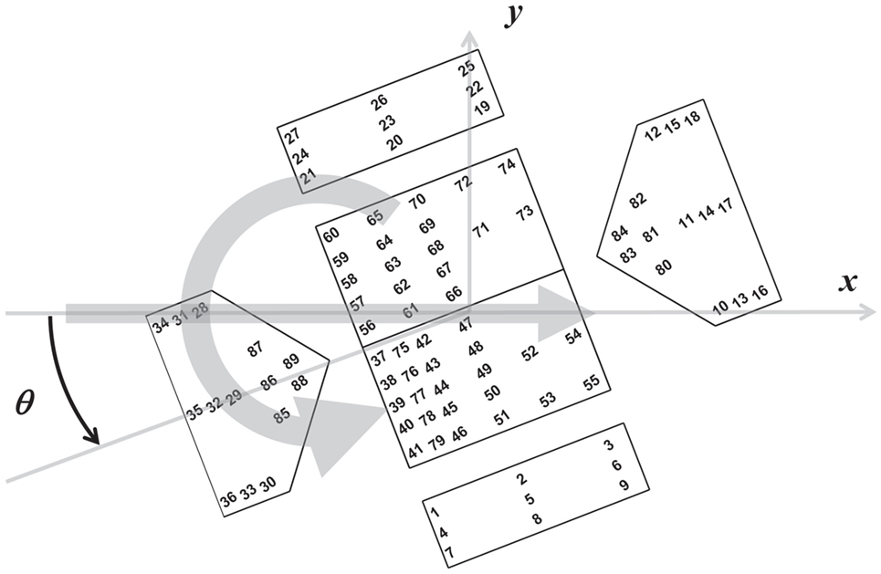
Figure 1. Building model schematic showing pressure tap numbering, the x and y direction definitions, and the approach angle (θ) definition. The large arrows indicate the translation and rotation directions of the vortex; the vortex translated through the center of the building for all tests.

Test Conditions

A single, low-swirl vortex was used for these tests (referred to as a Vane1 vortex in Haan et al., 2010). Pressures were acquired on the building with the vortex translating and stationary. Table 1 summarizes the test parameters, and the schematic diagram in Figure 2 defines notation and shows the arrangement of the measurement position relative to the tornado vortex.

TABLE 1

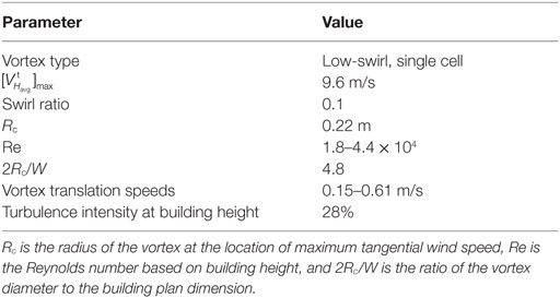
Table 1. Summary of parameters of the tornado-like vortex used in this study.

FIGURE 2

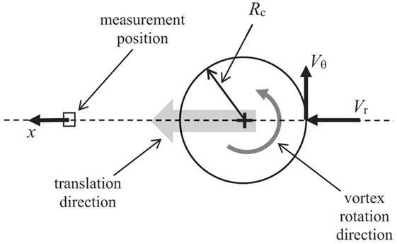
Figure 2. Schematic diagram showing the relationship between the vortex position and the measurement position.

Velocity measurements on this vortex were performed using a TFI Cobra probe located at the same measurement position as the model but with the model absent. The velocity measurements were conducted when the vortex was translating and when it was stationary. For the translating cases, five time series were acquired for each direction of the probe (because the probe can only acquire data within a 45° cone of acceptance, tests were run with the probe facing one way and then repeated with the probe turned around 180°). These time series were broken into 0.1-s segments. Within each segment, an average value and a peak value were computed. The nomenclature chosen for these two values was $V_{H_{\text{avg}}}^{\text{t}}$ and $V_{H_{\text{peak}}}^{\text{t}}$, respectively. The superscript t was used to denote the “translating” case, and the subscript H denotes horizontal velocity (the vector sum of the tangential and radial components of the vortex—denoted as V_θ and V_r, respectively, in Figure 2). The velocity data for both stationary and translating vortices are presented in Figure 3 as a function of position (x) with respect to the center of the vortex core. The x positions are normalized by the radius of the vortex core, R_c (see Table 1). The stationary data in Figure 3 (denoted by the superscript s) were found from 48 s of data at each x/R_c location. Each 48-s data set was divided into 1-s segments in which peak velocities were found. The data in Figure 3 represent the median of the resulting 48 peak values. More details on these velocity measurements can be found in Fleming et al.’s study (Fleming et al., 2013).

FIGURE 3

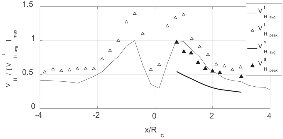
Figure 3. Horizontal velocity measurements for a translating and a stationary vortex. The lines represent local average velocities while the symbols are local peak velocities.

Values of $V_{H_{\text{avg}}}^{\text{t}}$ ranged from 4 to 10 m/s and were used (along with the building height) to estimate the Reynolds numbers of the building model tests. In this project, the Re values ranged from 1.8 × 10⁴ away from the core to 4.4 × 10⁴ at the core radius. It has conventionally been assumed that sharp-edged bluff body flows are relatively independent of Re effects for Re greater than ~3 × 10⁴.

The pressure and velocity tests considered in this paper involved vortex translation speeds from 0.15 to 0.61 m/s, and the pressure tests considered a single building orientation of 0° with respect to the vortex translation direction (see Figure 1 for angle definition). For translating cases, 10 passes of the vortex past the building were used to acquire pressure data. For stationary cases, 48 s of pressure data were acquired for a range of vortex distances from the building center (x = 0.4R_c − 2.4R_c). The analytical approach for obtaining peak pressure coefficients is described in the next section. It should also be noted that velocity measurements using the Cobra probe were conducted separately from the pressure measurements on the building. The measurements were not simultaneous.

Analytical Details on Peak Pressure Estimation

Figure 4 shows a single, illustrative pressure time series from roof tap #66 on the building model. This plot is a time series even though the horizontal axis has been transformed to show position of the vortex with respect to the center of the building. The figure also shows the vortex-induced static pressure $(C_{p_{\text{static}}}(x))$, the building orientation, and the rotation direction of the vortex. One method of finding peak pressure coefficients is to find the peak negative pressures from 10 of these time series, find the median of those peak negative pressures, and report the peak C_p using a dynamic pressure based on the maximum average horizontal velocity, ${[V_{H_{\text{avg}}}^{\text{t}}]}_{\text{max}}$, as shown in Eq. 1 below:

$C_{p_{\text{peak}}}=\frac{{\left(p-p_{\text{ref}}\right)}_{\text{peak}}}{\frac{1}{2}\mathrm{\rho }{\left[V_{H_{\text{avg}}}^{\text{t}}\right]}_{\text{max}}^2}$ (1)

where ρ is air density, p is pressure measured at the pressure tap on the building, and p_ref is the laboratory pressure far outside the vortex (the reference pressure). Using this method, tap #66 experiences $C_{p_{\text{peak}}}$ values of around −3.1. This is significantly higher than the ASCE 7–10 pressure coefficient of −1.2 for this location on the roof (ASCE, 2010). This approach to finding the peak is similar to that of Haan et al.’s study (Haan et al., 2010).

FIGURE 4

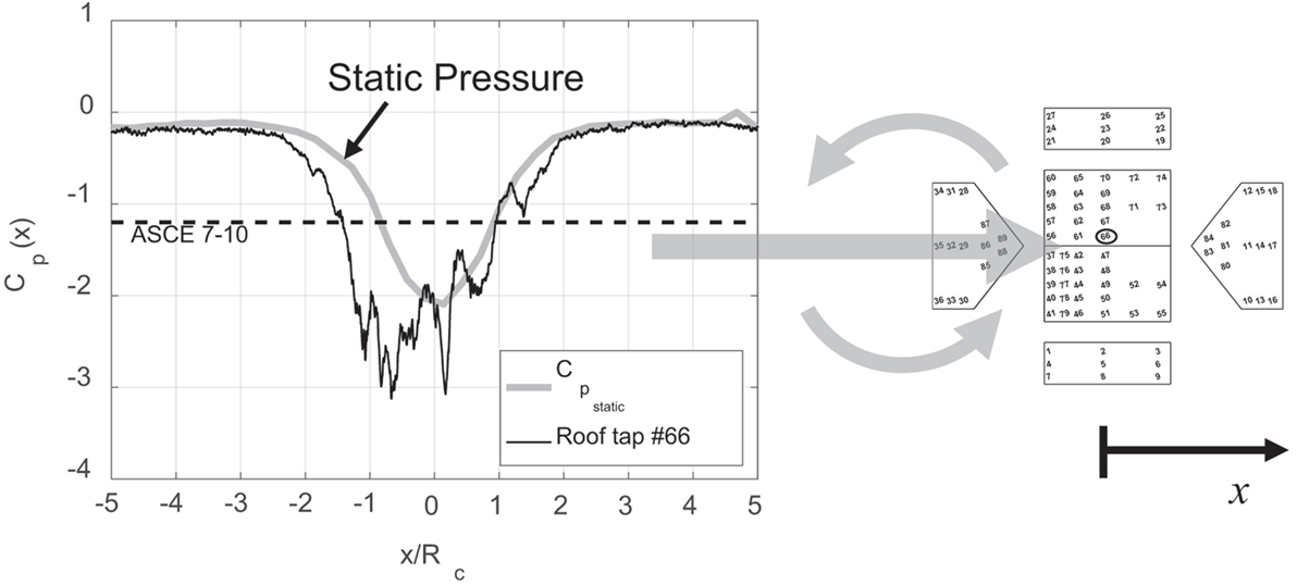
Figure 4. Example time series from a roof pressure tap (#66) as the vortex passes the building as well as the static pressure generated by the vortex. Pressure tap #66 is circled on the building model. The large arrows indicate the direction of translation and rotation of the vortex. Note that both pressure coefficients were computed using a dynamic pressure based on ${[V_{H_{\text{avg}}}^{\text{t}}]}_{\text{max}}$.

In the present study, a new approach was employed to determine the degree to which this large peak value comes from the vortex-induced static pressure in the core or from transient effects of the vortex passing. The intent was to strip away the static pressure and normalize the pressure to account for the transient velocity and see whether what remains could be considered equivalent to straight-line flow.

To implement this approach, the static pressure (as shown in Figure 4) was subtracted from the pressure signal to eliminate its role in generating large peaks. Also, the pressure peaks were normalized by a local velocity (following the velocity profile of Figure 3 rather than the maximum average velocity used in Eq. 1) to determine whether the vortex flow field itself plays a role in the large peaks. This approach can be formulated as shown in Eq. 2 below if one normalizes using the peak velocity:

$\begin{array}{c}{C}_{p_{\text{peak}}}\left(x\right)=\frac{{\left(p\left(x\right)-p_{\text{ref}}\right)}_{\text{peak}}}{\frac{1}{2}\mathrm{\rho }{\left[V_{H_{\text{peak}}}^{\text{t}}\left(x\right)\right]}^2}-\frac{p_{\text{static}}\left(x\right)-p_{\text{ref}}}{\frac{1}{2}\mathrm{\rho }{\left[V_{H_{\text{peak}}}^{\text{t}}\left(x\right)\right]}^2}=\frac{{\left(p\left(x\right)-p_{\text{ref}}\right)}_{\text{peak}}}{\frac{1}{2}\mathrm{\rho }{\left[V_{H_{\text{peak}}}^{\text{t}}\left(x\right)\right]}^2}-C_{p_{\text{static}}}\left(x\right)\end{array}$ (2)

where ${\left(p\left(x\right)-p_{\text{ref}}\right)}_{\text{peak}}$ is the peak pressure as a function of x computed over each of the 0.1-s time segments described in Section “Test Conditions.” p_static(x) − p_ref is the static pressure induced by the vortex and measured by averaging together all 89 building pressure taps for each time step. This vortex-induced static pressure was also measured using floor taps with the building absent and using the Cobra probe with the building absent. All three methods produced the same static pressure curve.

Results and Discussion

Peak Pressures from Adjusted Pressure Signals

Adjusting the pressure signals as represented by Eq. 2 produces the $C_{p_{\text{peak}}}(x)$ profiles presented in Figure 5. This figure shows peak pressure profiles made using both $V_{H_{\text{avg}}}^{\text{t}}(x)$ and $V_{H_{\text{peak}}}^{\text{t}}(x)$ values and a line indicating the peak pressure provision of ASCE 7–10 for this roof location. Given the transient nature of the tornado, it is not clear which velocity would make for a more appropriate comparison with ASCE 7–10. Normalizing with local peak pressures brought the $C_{p_{\text{peak}}}(x)$ profile within the standard provisions. Further results in this study were all normalized with local peak velocity.

FIGURE 5

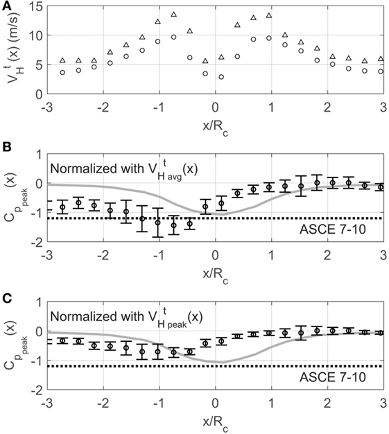
Figure 5. (A) Horizontal velocity values from translating tests averaged over 0.1-s time intervals as the vortex passes. (B) Peak pressure coefficients from translating tests for tap #66 computed by subtracting static pressure, finding peaks in 0.1-s intervals, and normalizing with a dynamic pressure based on the local value of $V_{H_{\text{avg}}}^{\text{t}}(x)$. (C) Same as panel (B) except normalized with a dynamic pressure based on the local value of $V_{H_{\text{peak}}}^{\text{t}}(x)$. Circles represent the median peak value and error bars represent 95% confidence intervals. The dashed line denotes the −1.2 peak pressure suggested by ASCE 7–10 for this roof location. The gray line is the static pressure.

At the edge of the core and just outside it, peak pressures are greatest as are the confidence intervals for those peak pressures. A flat trend here would suggest that the aerodynamics outside the core might be fundamentally similar to straight-line flow if we simply account for the horizontal velocity being a function of distance from the core. Since the $C_{p_{\text{peak}}}(x)$ values do not follow a flat trend, the idea that we have basically straight-line flow along with a static pressure adjustment appears too simplistic.

It should be noted that within the core, $C_{p_{\text{peak}}}(x)$ values produced by Eq. 2 would grow very large because the horizontal velocity decreases greatly there. Rather than artificially inflating pressure coefficients there, $C_{p_{\text{peak}}}(x)$ values for −1 < x/R_c < 1 were normalized using the maximum value of $V_{H_{\text{peak}}}^{\text{t}}(x)$.

Duration Effects

Two different approaches were used to study duration effects. Comparing pressure peaks from stationary vortex events and from translating vortex events were the first method used to study the role of event duration in pressure peak generation. A set of data was acquired for a stationary vortex at various positions relative to the building. Since the translation speed of the tests included in this study were the fastest possible with the ISU simulator, the translating and stationary data sets presented here represent the shortest and longest durations that could be studied.

Figure 6 shows $C_{p_{\text{peak}}}(x)$ profiles for tap 66 from these translating and stationary vortex tests. The stationary test coefficients were all computed by subtracting static pressure, finding peaks in 1.0-s intervals, and normalizing with a dynamic pressure based on the same local value of $V_{H_{\text{peak}}}^{\text{t}}(x)$ used to normalize the translating data (using the maximum value of $V_{H_{\text{peak}}}^{\text{t}}(x)$ for locations inside the core as described in Section “Peak Pressures from Adjusted Pressure Signals”).

FIGURE 6

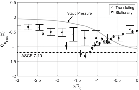
Figure 6. Peak pressure coefficients for tap #66 from translating test (as in Figure 7) and also from stationary vortex tests. Error bars are 95% confidence intervals. The dashed line denotes the −1.2 peak pressure suggested by ASCE 7–10 for this roof location.

The stationary vortex peaks were significantly larger than the translating vortex peaks suggesting that a vortex that spends more time on a given building would generate larger peaks pressures. The largest stationary vortex peaks have magnitudes 45% larger than the translating vortex peaks. Test results like this using stationary vortices might represent an envelope for the peak pressures one can expect on a building, that is, in the worst case, when the vortex sits on a building without moving at all. To obtain a true envelope for such pressures; however, more parameters would need to be considered. For example, the diameter of the vortex in this case is about five times the building plan dimension. Testing how this ratio affects peak pressures would also need to be done.

The second method of studying event duration was to observe changes in peak pressures as a function of vortex translation speed. This was done somewhat in Haan et al.’s study (Haan et al., 2010), but here it is done in a different form. In this study, a comparison was made between peaks found from stationary vortex pressure time series divided into segments of various lengths (to simulate various durations) and peaks from translating vortex pressure time series where the durations occur naturally given the transient nature of the tests.

For the translating vortex cases, the duration of the vortex event was estimated as the time that a point on the building is exposed to the vortex core, that is, the time it takes the vortex to translate past a single point. The duration, τ, then was estimated as follows in Eq. 3:

$\mathrm{\tau }=\frac{2R_{\text{c}}}{V_{\text{t}}}$ (3)

where V_t is the vortex translation speed. With this study’s translation speeds of 0.15–0.61 m/s, this resulted in duration values from 0.7 to 2.9 s. Each translation speed was tested 10 times, peak C_p values were found for each of these 10 trials. A median peak value was found for the 10 trials for each translation speed.

For the stationary vortex cases, data were divided in a manner similar to that employed by Kopp and Morrison (2011). The 48 s of each stationary vortex time series was divided into segments as long as 10 s and as short as 0.1 s. Given the nature of turbulent flow pressure fluctuations, the longer time segments should result in larger peak pressures. The peak C_p was obtained for each segment and the median C_p was found for the entire 48 s time series.

All the peak values from various segment lengths (for both stationary and translating cases) were then normalized with the median C_p of the entire 48 s. stationary vortex time series. The resulting peak to median ratio for tap 66 is plotted as a function of duration in Figure 7. The data show that as duration increases, the peak to median ratio increases as well. In the next section, peak/median ratios are presented for all the pressure taps, and overall trends with respect to duration are discussed.

FIGURE 7

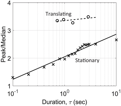
Figure 7. Ratio of peak C_p to median C_p as a function of event duration, τ, for translating and stationary vortex tests on pressure tap #66.

All Pressure Taps

The analyses already presented for tap 66 were also conducted for all 89 taps on the building model. To present these results in a concise manner, the pressure taps were organized according to zones as shown in Figure 8. These zones were chosen based on similarity of pressure peak behavior. Figure 9 shows envelope curves for $C_{p_{\text{peak}}}(x)$ values for all the building’s pressure taps. To generate these envelope curves, the plots shown in Figure 6 were made for all the pressure taps in a given zone. The envelope curves represent the upper and lower bounds of all the 95% confidence intervals of those pressure taps. As was the case with tap 66, the stationary vortex peak values have larger magnitudes than the translating vortex values. An important thing to note is that the stationary data were not acquired for the entire positive and negative x/R_c range. This means that for some tap zones, the worst case vortex positions were not sampled. This is true for zones 3–7 and 14–15.

FIGURE 8

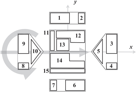
Figure 8. Pressure tap zone definitions for organizing the pressure taps shown in Figure 3. These zones are used for presenting the results of peak C_p and duration analysis in Figures 9 and 10.

FIGURE 9

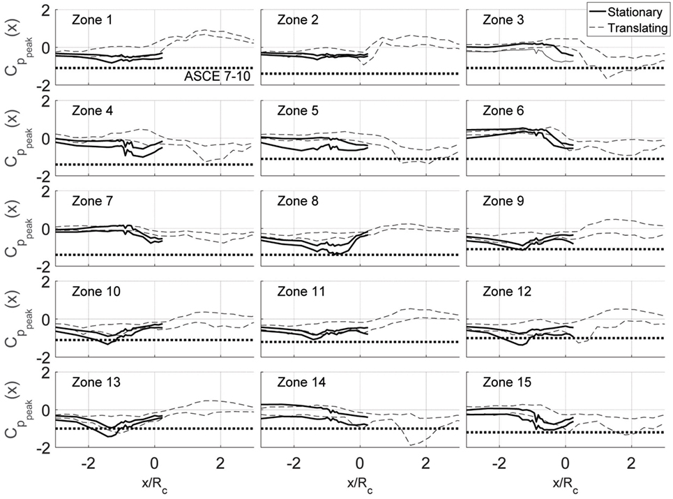
Figure 9. Envelope curves for $C_{p_{\text{peak}}}(x)$ values for all pressure taps for both stationary and translating vortex tests. Zones correspond to the definitions in Figure 8. ASCE 7–10 provisions are provided for each zone. Note: these zones do not coincide with ASCE 7–10 zones. The lines shown here represent the smallest magnitude ASCE 7 value for any tap in the zone.

The ASCE 7–10 values are represented in Figure 9 as well; however, the zones defined in Figure 8 do not coincide with ASCE 7–10 zones. The lines in Figure 9 then represent the smallest magnitude ASCE 7 value for any tap in the zone. To summarize the trends of the figure, ratios between the $C_{p_{\text{peak}}}(x)$ values and the ASCE 7–10 provisions are presented in Table 2. All the shaded entries in the table are those which exceed the ASCE 7 provisions. In the case of zone 14, the peak values exceed ASCE 7 by 89%. Two things are worthy of mentioning in Table 2. The first is that, as expected, the stationary values have typically larger magnitudes than the translating values. The second is that these values in Table 2 should not be used as conversion factors from ASCE 7 to tornado values because the actual pressure coefficients acting on the building model must still include a static pressure component. As discussed later in Section “Comparing Time Series of Stationary and Translating Data,” the static pressure cannot simply be added to the values in Table 2 to recover original peak pressure coefficients.

TABLE 2

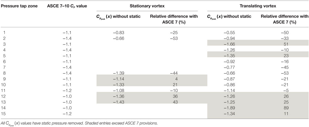
Table 2. Summary table of $C_{p_{\text{peak}}}(x)$ values for all pressure tap zones.

The duration analysis of Section “Duration Effects” was also applied to all the pressure taps. The results are shown in Figure 10 arranged according to zones. Those zones where the worst case vortex positions were not sampled with stationary data (3–7, 14–15) were omitted from this figure. The translating results are often too scattered to make conclusive statements, but the rough trends with duration are clear. Increasing duration increases peak pressure magnitudes. To quantify these trends, the following expression was used to fit these data:

$\text{PM}=m\text{\hspace{0.17em}ln(}\mathrm{\tau }\text{)}+b$ (4)

where PM is the peak/median ratio presented in Figures 7 and 10 and m and b are fit constants.

FIGURE 10

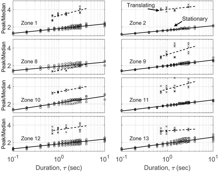
Figure 10. Peak C_p to median C_p ratios as a function of event duration, τ, for every pressure tap as organized into the zones defined in Figure 8. Translating and stationary vortex test results are included.

The fit constants, m and b, are presented in Table 3 for each zone. To tabulate how much peak C_p values would change with duration, the PM expression of Eq. 4 was used to compute a ratio of the peak/median values for τ values of 100 and 10 s. Depending on the zone, the factors between peak values at 100 s and those at 10 s are 1.1–1.4. These ratios are similar to what Kopp and Morrison (2011) found using pressures from a building in an atmospheric boundary layer (ABL).

TABLE 3

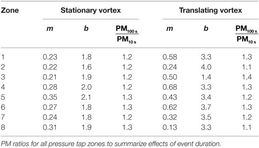
Table 3. Fit parameters and 100–10 s.

Analysis like this could result in a factor that could be used to adjust tornado pressure coefficients for events of different duration.

Velocity and Static Pressure Profiles

The previous two sections presented data showing that peak pressures generated by tornado vortices can be larger than those from straight-line turbulent boundary layer flow. The cause for some of the differences probably lies with the unsteady effects observed in the vertical velocity and the vortex-induced static pressure. Figure 11A shows the vertical velocity profile normalized with the maximum horizontal velocity. When the vortex was translating, the instantaneous velocity peaks were observed to be three times as large as the average values and up to 75% of the horizontal velocity. For the stationary vortex, the peaks were four times are large as the means and equal to the horizontal velocity. Unsteadiness like this near the core was also observed for the static pressure as presented in Figure 11B. Although the analysis in this paper removed the average static pressure (the solid lines in Figure 11B and gray lines in Figures 4–6) from the building pressure tap signal, the static pressure fluctuates about that average. These fluctuations would affect the building envelope. Figure 11B shows peaks in the static pressure 25% higher than the average.

FIGURE 11

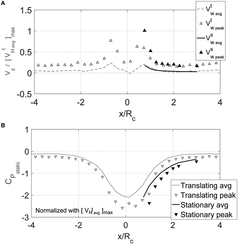
Figure 11. (A) Vertical velocity measurements for the vortex when translating and stationary. Superscripts “t” and “s” denote translating and stationary tests, respectively. All velocities are normalized by the maximum horizontal velocity observed for the translating vortex, $C_{p_{\text{peak}}}(x)$. (B) Vortex-induced static pressure for the vortex when translating and stationary. All pressures were normalized using a dynamic pressure based on the maximum horizontal velocity observed for the translating vortex, ${[V_{H_{\text{avg}}}^{\text{t}}]}_{\text{max}}$.

Comparing Time Series of Stationary and Translating Data

Another way to illustrate the unique contribution of the static pressure on tornado-induced loading is shown in Figure 12 where time series of pressure coefficients are shown for several translating vortex tests and a stationary vortex test. One interesting observation is the significant difference static pressure makes in the two types of signals. For these stationary data, removing the static pressure is simply an offset to the whole signal. In the translating cases, the peaks in the signals are drastically reduced. If the two signals are compared while including static pressure, the translating data show peaks of larger magnitude. If the static pressure is removed, the stationary data have the larger magnitude peaks. How the static pressure and the peak pressure events do or do not correlate with each other is worthy of more study.

FIGURE 12

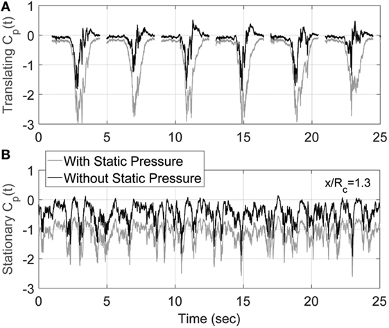
Figure 12. Time series of the pressure coefficient at tap #66 for (A) translating vortex—six vortex events have been plotted together here to illustrate the variability of the signal, (B) stationary vortex at x/R_c = 1.3. Each time series is presented with and without static pressure.

The large stationary-vortex peak events of Figure 12 might suggest that the vortex is oscillating in space somewhat and impinging on the structure over and over. The nature of the time series should be investigated further. This might require capturing a time-resolved vortex velocity field (such as with a high-speed PIV system) simultaneous to building pressure measurements. While the results of this project show some of the distinctive attributes of tornado-induced pressures, a very interesting future study would involve simultaneous measurements of velocity and pressure such that the spatiotemporal relationships among vertical gusts, static pressure fluctuations, and the pressure peaks on the building surface could be illuminated further.

Conclusion

This study investigated the role of tornado-induced static pressure and duration on peak pressures on a low-rise building. Past studies have suggested that peak pressures on buildings in tornadoes were up to 50% (or more) higher than straight-line ABL values (Haan et al., 2010). This study showed that much, but not all, of this increase can be explained by the static pressure of the vortex. While subtracting the static pressure from pressure time series and normalizing by a local horizontal peak velocity brought peak pressures closer to what one would expect from straight-line ABL flows, the data showed that peaks in some portions of the building could still be as much as 90% larger the ASCE 7–10 provisions.

To consider duration effects, pressure peak results from both translating vortex and stationary vortex tests were considered. Increases in duration were found to increase peak pressure coefficient magnitudes. Depending on the zone of the building, changing duration from 10 to 100 s was found to increase peak magnitudes by factors of 1.1–1.4. Work such as this might lead to factors that could adjust tornado pressure coefficients for the effect of event duration.

Both the stationary and the translating vortex pressure peaks were observed to occur in or near the vortex core, and profiles of vertical velocity and static pressure suggest that strong unsteady vertical gusting and strong static pressure fluctuations could play a role in creating these larger stationary-vortex peaks. The pressure time series resulting from these phenomena showed that removing the static pressure had a more significant effect on the translating vortex pressure signals than on the stationary vortex pressure. This indicates the significance of the correlation/timing between the static pressure and velocity-induced pressures. This is worthy of further investigation.

While this project investigated the results from a single vortex type, future work must investigate the effects of other tornado parameters such as tornado diameter relative to building size and tornado structure as controlled by swirl ratio.

Author Contributions

The corresponding author was responsible for the design of the experiments for this project, for acquiring these data, for conducting the analysis, and writing the manuscript. The corresponding author is accountable for all aspects of the work in ensuring that questions related to the accuracy or integrity of any part of the work are appropriately investigated and resolved. The author gratefully acknowledges the contributions of Partha P. Sarkar to the conception, design, and construction of the facility used for this work and the contributions of graduate assistants Vasanth Balaramudu and Mark Fleming for their work acquiring these data.

Conflict of Interest Statement

The author declares that the research was conducted in the absence of any commercial or financial relationships that could be construed as a potential conflict of interest.

Acknowledgments

The author gratefully acknowledges the work of Bill Rickard and numerous undergraduate students from the Iowa State Aerospace Engineering Department who contributed to this project.

Funding

This work was sponsored by the U.S. National Science Foundation under grants 0220006 and 0239070.

References

ASCE. (2010). Minimum Design Loads for Buildings and Other Structures. Reston, VA: American Society for Civil Engineers.

Google Scholar

Chang, C. C. (1971). “Tornado wind effects on buildings and structures with laboratory simulation,” in Proceedings of the 3rd International Conference on Wind Effects on Buildings and Structures, Tokyo, 231–240.

Google Scholar

Fleming, M. R., Haan, F. L. Jr., and Sarkar, P. P. (2013). Turbulent Structure of Tornado Boundary Layers with Translation and Surface Roughness. 12th America’s Conference on Wind Engineering. Seattle, WA.

Google Scholar

Haan, F. L. Jr., Balaramudu, V. K., and Sarkar, P. P. (2010). Tornado-induced wind loads on a low-rise building. J. Struct. Eng. 136, 106–116. doi: 10.1061/(ASCE)ST.1943-541X.0000093

CrossRef Full Text | Google Scholar

Haan, F. L. Jr., Sarkar, P. P., and Gallus, W. A. (2008). Design, construction and performance of a large tornado simulator for wind engineering applications. Eng. Struct. 30, 1146–1159. doi:10.1016/j.engstruct.2007.07.010

CrossRef Full Text | Google Scholar

Jischke, M. C., and Light, B. D. (1983). Laboratory simulation of tornadic wind loads on a rectangular model structure. J. Wind Eng. Ind. Aerodyn. 13, 371–382. doi:10.1016/0167-6105(83)90157-5

CrossRef Full Text | Google Scholar

Kikitsu, H., Sarkar, P. P., and Haan, F. L. (2011). “Experimental study on tornado-induced loads of low-rise buildings using a large tornado simulator,” in 13th International Conference on Wind Engineering (Amsterdam, Netherlands).

Google Scholar

Kopp, G. A., and Morrison, M. J. (2011). Discussion of “tornado-induced wind loads on a low-rise building” by F.L. Haan Jr., V.K. Balaramudu, and P.P. Sarkar. J. Struct. Eng. 137, 1620–1624. doi:10.1061/(ASCE)ST.1943-541X.0000309

CrossRef Full Text | Google Scholar

Kosiba, K., and Wurman, J. (2013). The three-dimensional structure and evolution of a tornado boundary layer. Weather Forecasting 28, 1552–1561. doi:10.1175/WAF-D-13-00070.1

CrossRef Full Text | Google Scholar

Mishra, A. R., James, D. L., and Letchford, C. W. (2008). Physical simulation of a single-celled tornado-like vortex, part B: wind loading on a cubic model. J. Wind Eng. Ind. Aerodyn. 96, 1258–1273. doi:10.1016/j.jweia.2008.02.063

CrossRef Full Text | Google Scholar

Refan, M., and Hangan, H. (2016). Characterization of tornado-like flow fields in a new model scale wind testing chamber. J. Wind Eng. Ind. Aerodyn. 151, 107–121. doi:10.1016/j.jweia.2016.02.002

CrossRef Full Text | Google Scholar

Sabareesh, G. R., Matsui, M., and Tamura, Y. (2013a). Characteristics of internal pressure and resulting roof wind force in tornado-like flow. J. Wind Eng. Ind. Aerodyn. 112, 52–57. doi:10.1016/j.jweia.2012.11.005

CrossRef Full Text | Google Scholar

Sabareesh, G. R., Matsui, M., and Tamura, Y. (2013b). Ground roughness effects on internal pressure characteristics for buildings exposed to tornado-like flow. J. Wind Eng. Ind. Aerodyn. 122, 113–117. doi:10.1016/j.jweia.2013.07.010

CrossRef Full Text | Google Scholar

Wurman, J., Kosiba, K., and Robinson, P. (2013). In situ, Doppler radar, and video observations of the interior structure of a tornado and the wind-damage relationship. Am. Meteorol. Soc. 94, 835–846. doi:10.1175/BAMS-D-12-00114.1

CrossRef Full Text | Google Scholar