Automatic Kernel Selection for Gaussian Processes Regression with Approximate Bayesian Computation and Sequential Monte Carlo

1. Introduction and Motivation

Regression analysis or classification using Bayesian formulation and specifically Gaussian Processes (GPs) or relevance vector machines (RVMs) is becoming very popular and attractive due to incorporation of uncertainty and the bypassing of unattractive features from methods like neural networks. Regression using neural networks for example, although they present a very powerful tool, sometimes can make it difficult and demanding to achieve the right tuning. The hard questions that have to be asked while multi-layer perceptrons (MLPs) are implemented are: which is the right architecture? How many nodes? What transfer functions? What momentum or learning rate? How many times they should run for different initial conditions?

The use of Gaussian processes is a current research area of increasing interest, not only for regression but also for classification purposes (Dervilis et al., 2015). Gaussian processes (GPs) are a stochastic non-parametric Bayesian approach to regression and classification problems. These Gaussian processes are computationally very efficient, and non-linear learning is relatively easy. Gaussian process regression takes into account all possible functions that fit to the training data vector and gives a predictive distribution around a single prediction for a given input vector. A mean prediction and confidence intervals on this prediction can be calculated from the predictive distribution. Due to its simplicity and desirable computational performance, GP has been applied in numerous domains particularly in structural health monitoring (Cross, 2012; Dervilis et al., 2016; Worden and Cross, 2018) and civil and structural engineering to construct surrogate models, which can mimic the real behavior of large-scale complex systems/structures and then make predictions. In Su et al. (2017), GP model has been coupled with Monte Carlo simulations to perform a reliability analysis of complex engineering structures. An application of GP to control an existing building can be found in Ahn et al. (2015). In Wan et al. (2014), a surrogate model based on GP has been established to deal with uncertainty quantification for modal frequencies. An interesting application of GP to deal with finite element model updating for a civil structures is presented in Wan and Ren (2015).

The initial and basic step in order to apply Gaussian process regression is to obtain a mean and covariance function. These functions are specified separately, and consist of a specification of a functional form and a set of parameters called hyperparameters. When the mean and covariance functions are specified, then one can infer model hyperparameters by minimization of the log-marginal likelihood. The software used for the implementation of GP regression was provided by Rasmussen and Williams (2006).

However, as mentioned, a covariance or kernel function has to be defined and the new questions that one has to ask: how one chooses the kernel function for a GPs? And of course one could say, well the people running or providing the code are experts on GPs why they do not include a default mechanism to choose kernel and it is user oriented and free choice?

The answer is that the choice of any covariance function or kernel, determines in the authors opinion, almost all the generalization properties of GPs, but here one is talking about a black box model and the user might not be an expert, or not have a deep data or physics understanding or the modeling challenge. In turn, if one is not qualified to choose the proper covariance function as an expert, then this work is adding an important practical and sophisticated approach in order to choose a sensible kernel.

The article starts out with an introduction to the GPs and approximate Bayesian computation based on Sequential Monte Carlo (ABC-SMC) algorithm and the selection of the different hyperparameters required for its implementation. Then, in Section Simple Demonstration Example, the application of the ABC algorithm is illustrated and investigated through two illustrative examples using simulated and real data and forms the core of the article. Finally, the article is closed with some conclusions about the strengths of the method and future discussion.

2. Gaussian Processes (GP)

Rasmussen and Williams (2006) define a Gaussian process (GP) as “a collection of random variables, any finite number of which have a joint Gaussian distribution.” In recent years, GPs are gaining a lot of attention in the area of regression (or classification) analysis as they offer fast and simple computation properties (Dervilis, 2013). The core of the algorithm is coming from Rasmussen and Williams (2006).

2.1. Algorithm Theory

The initial step in order to apply Gaussian process regression is to define a prior mean m({x}) and covariance function k({x},{x′}), as GPs are completely specified by them, {x} represents the input vector. For any real process f ({x}) one can define:

$m\left(\left\{x\right\}\right)=E\left[f\left(\left\{x\right\}\right)\right]$ (1)

$k\left(\right\{x\},\{x^{\prime }\left\}\right)=E\left[\right(f\left(\right\{x\left\}\right)-m\left(\right\{x\left\}\right)\left)\right(f\left(\right\{x^{\prime }\}-m(\left\{x^{\prime }\right\}\left)\right]$ (2)

where E represents the expectation. Often, for practical reasons, because of notation purposes (simplicity), and lack of prior knowledge for the overall trend of the data, the prior mean function is set to zero. The Gaussian processes can then be defined as

$f\left(\left\{x\right\}\right)\sim \mathit{GP}\left(0,k\left(\left\{x\right\},\left\{x^{\prime }\right\}\right)\right).$ (3)

Assuming a zero-mean function, the covariance function could be described as

$\begin{array}{ll}\hfill \text{cov}\left(f\left({\left\{x\right\}}_p\right),f\left({\left\{x\right\}}_q\right)\right)& =k\left({\left\{x\right\}}_p,{\left\{x\right\}}_q\right)\\ & ={\sigma }^2\text{exp}\left(-\frac{1}{2}{∥{\left\{x\right\}}_p-{\left\{x\right\}}_q∥}^2\right).\end{array}$ (4)

This is the squared-exponential covariance function (although not the only option). It is very important to mention an advantage of the previous equation as the covariance is written as a function only of the inputs. For the squared-exponential covariance, it can be noted that it takes nearly unit values between variables where their inputs are very close and starts to decrease as the variable distance in the input space increases.

Assuming now that one has a set of training outputs {f } and a set of test outputs ${\left\{\mathit{\text{f}}\right\}}_{\ast }$ one has the prior:

$\left[\begin{array}{c}\hfill \left\{f\right\}\hfill \\ \hfill {\left\{f\right\}}_{\ast }\hfill \end{array}\right]\sim N\left(0,\left[\begin{array}{cc}\hfill K\left(X,X\right)\hfill & \hfill K\left(X,X_{\ast }\right)\hfill \\ \hfill K\left(X_{\ast },X\right)\hfill & \hfill K\left(X_{\ast },X_{\ast }\right)\hfill \end{array}\right]\right)$ (5)

where the capital letters represent matrices. A zero-mean prior has been used for simplicity, and K(X, X) is a matrix whose i,jth element is equal to k(x_i, x_j). And K(X, X_*) is a column vector whose ith element is equal to k(x_i; x_*), and K(X_*, X) is the transpose of the same. The covariance matrix must be symmetrical about the main diagonal.

As the prior has been generated by the mean and covariance functions, in order to specify the posterior distribution over the functions, one needs to limit the prior distribution in such a way that it includes only these functions that agree with actual data points. An obvious way to do that is by generating functions from the prior and selecting only the ones that agree with the actual points. Of course, this is not a realistic way of doing it as it would consume a lot of computational power. In a probabilistic manner, the operation can be done easily via conditioning the joint prior on the observations and this will give (for more details see Bishop (1995), Nabney (2002), and Rasmussen and Williams (2006)):

$\begin{array}{ll}& {\left\{f\right\}}_{\ast }|{\left[X\right]}_{\ast },\left[X\right],\left\{f\right\}\\ & \sim N\left(\begin{array}{c}K\left(\left[X_{\ast }\right],\left[X\right]\right)K{\left(\left[X\right],\left[X\right]\right)}^{-1}\left\{f\right\},K\left(\left[X_{\ast }\right],\left[X_{\ast }\right]\right)\\ -K\left(\left[X_{\ast }\right],\left[X\right]\right)K{\left(\left[X\right],\left[X\right]\right)}^{-1}K\left(\left[X\right],\left[X_{\ast }\right]\right)\end{array}\right).\end{array}$ (6)

Function values ${\left\{\mathit{\text{f}}\right\}}_{\ast }$ can be generated by sampling from the joint posterior distribution and at the same time evaluating the mean and covariance matrices from equation (6).

The covariance functions used in this study are usually controlled by some hyperparameters in order to obtain a better control over the types of functions that are considered for the inference. One of the most commonly employed kernels for GPs is the squared-exponential covariance function, which can take the following form:

$k_y\left(x_p,x_q\right)={\sigma }_f^2\text{exp}\left(-\frac{1}{2l^2}{\left(x_p-x_q\right)}^2\right)+{\sigma }_n^2{\delta }_{\mathit{pq}}$ (7)

where k_y is the covariance for the noisy target set y (i.e., y = f ({x}) + ε, where {x} is input vector and ε is the noise). The length scale l (determines how far one needs to move in input space for the function values to become uncorrelated), the variance ${\sigma }_f^2$ of the signal and the noise variance ${\sigma }_n^2$ are free parameters that can be varied. These free parameters are called hyperparameters.

The tool that is usually applied for choosing the optimal hyperparameters for GP regression is the maximum marginal likelihood of the predictions p({y}|[X], {θ}) with respect to the hyperparameters θ:

$\begin{array}{ll}\hfill \mathrm{\text{log\hspace{0.17em}}}p\left(\left\{y\right\}|\left[\text{X}\right],\left\{\theta \right\}\right)& =-\frac{1}{2}{\left\{y\right\}}^T{\left[K\right]}_y^{-1}\left\{y\right\}-\frac{1}{2}\log \left|\left[K_y\right]\right|-\frac{n}{2}\log 2\pi \end{array}$ (8)

where $\left[K_y\right]=\left[K_f\right]+{\sigma }_n^{2}I$ is the covariance matrix of the noisy test set {y} and [K_f] is the noise-free covariance matrix. In order to optimize these hyperparameters through maximizing the marginal log likelihood, the partial derivatives give the solution, via gradient descent:

$\begin{array}{ll}\hfill \frac{\partial }{\partial {\theta }_j}\mathrm{\text{log\hspace{0.17em}}}p\left(\left\{y\right\}|\left[X\right],\left\{\theta \right\}\right)& =\frac{1}{2}{\left\{y\right\}}^T{\left[K\right]}^{-1}\frac{\partial \left[K\right]}{\partial {\theta }_j}{\left[K\right]}^{-1}\left\{y\right\}-\frac{1}{2}\mathit{tr}\left({\left[K\right]}^{-1}\frac{\partial \left[K\right]}{\partial {\theta }_j}\right)\\ & =\frac{1}{2}\mathit{tr}\left(\left(\alpha {\alpha }^T-{\left[K\right]}^{-1}\right)\frac{\partial \left[K\right]}{\partial {\theta }_j}\right)\end{array}$ (9)

where {α} = [K]^–1{y}. Of course this solution is not a trivial procedure, and for specific details, readers are referred to Rasmussen and Williams (2006).

3. Approximate Bayesian Computation (ABC)

As stated in the previous section, by default GPs need a selection of a kernel which for either SI or SHM might be of great interest as it may affect not only the mean prediction and actual accuracy but also the confidence bounds of the prediction. This creates a model selection and comparison problem, especially when several competing models—kernels in our case (or even expanded to the mean function)—are consistent with the selection criterion and could potentially explain the data reasonably well (this will be expanded later in the section Discussion).

In reality, selecting the most likely model or kernel among a family of competing models (big or small) may be quite challenging, especially with black box methods where deep understanding of the physics is not obvious.

Several methods have been proposed in the literature, and someone can start from Markov chain Monte Carlo (MCMC) variants to evolutionary algorithms like genetic algorithms or particle swarm. The reader can refer to the following references: Schwarz et al. (1978), Bishop (1995), Green (1995), Kullback (1997), Akaike (1998), Doucet et al. (2000, 2001), Au and Beck (2001), Nabney (2002), Lawrence (2003), Marjoram et al. (2003), Ching et al. (2006), Rasmussen and Williams (2006), Skilling (2006), Gretton et al. (2007), Beaumont et al. (2009), Toni et al. (2009), Toni and Stumpf (2010), Barnes et al. (2011), Worden et al. (2011), Neath and Cavanaugh (2012), Turner and Van Zandt (2012), Filippi et al. (2013), Hensman et al. (2013), Wilson and Adams (2013), Chiachio et al. (2014), Ben Abdessalem et al. (2016), and the references therein, where many varied examples illustrating the use of the Bayesian method are investigated. As GPs are an elegant Bayesian method, it fits very well to adopt a Bayesian approach for kernel selection and hyperparameter estimation as this shall give some uncertainty evaluation around the kernel parameters as well.

In this contribution, the approximate Bayesian computation (ABC) algorithm is used for the first time in order to deal with kernel selection and hyperparameter estimation. ABC offers a series of advantages over MCMC (or reversible jump MCMC (RJMCMC) in this context (Green, 1995)). ABC is as general as a Bayesian method can be as there is no need to evaluate any extra criterion to discriminate between competing kernels and the inference can be calculated for any different number of suitable metric regarding the similarity between the observed and modeled data, bypassing issues associated with intractable likelihood functions and Gaussian assumptions, which are not always valid.

Another major advantage offered by the ABC algorithm is its independence of the dimensionality of the competing model, as ABC is able to jump between the different kernel hyperparameter spaces without any need of a specific mapping function that assures continuing of dimension; this is a critical advantage when dealing with large numbers of kernels with different dimensions. In practice, the ABC algorithm compares the competing models simultaneously and eliminates progressively the least likely models, to converge to the most appropriate ones. For much deeper evaluation of ABC, the reader is referred to Toni et al. (2009) and Ben Abdessalem et al. (2016, 2017).

3.1. Quick Overview of ABC Algorithm

For a deep and detailed analysis of the algorithm, the reader is redirected to Schwarz et al. (1978), Bishop (1995), Green (1995), Kullback (1997), Akaike (1998), Doucet et al. (2000, 2001), Au and Beck (2001), Nabney (2002), Lawrence (2003), Marjoram et al. (2003), Ching et al. (2006), Rasmussen and Williams (2006), Skilling (2006), Gretton et al. (2007), Beaumont et al. (2009), Toni et al. (2009), Toni and Stumpf (2010), Barnes et al. (2011), Worden et al. (2011), Neath and Cavanaugh (2012), Turner and Van Zandt (2012), Filippi et al. (2013), Hensman et al. (2013), Chiachio et al. (2014), and Ben Abdessalem et al. (2016) as the purpose of this work is not to repeat the great advantages and theory behind ABC-SMC, but for the readers’ convenience, a brief introduction is given.

In the ABC algorithm, the objective is to obtain a “proper” and computationally efficient approximation to the posterior distribution:

$\pi \left(\xi |u^{\ast },\mathcal{M}\right)\propto f\left(u^{\ast }|\xi ,\mathcal{M}\right)\pi \left(\xi |\mathcal{M}\right)$ (10)

where $\mathcal{M}$ is the model based on a set of parameters (or kernel function) {ξ}, $\pi \left(\xi \right|\mathcal{M})$ denotes the prior distribution over the parameter space, and $f\left(u^{\ast }|\xi ,\mathcal{M}\right)$ is the likelihood of the observed data u* for a given parameter set {ξ}.

To overcome the issue of intractable likelihood functions, the ABC algorithm bypasses the problem by utilizing systematic comparisons between observed and output data. The main objective consists of comparing the simulated data, u, with observed data u*, and accepting simulations if a suitable distance measure between them, Δ(u, u*), is less than a specified threshold defined by the user, ε (for more information check Toni and Stumpf (2010) and Ben Abdessalem et al. (2016, 2017)). The ABC algorithm, as a result, gives a sample from the approximate posterior of the form

$\begin{array}{ll}\hfill \pi \left(\xi |u^{\ast },\mathcal{M}\right)\approx {\pi }_{\epsilon }\left(\xi |u^{\ast },\mathcal{M}\right)\propto & \int f\left(u^{\ast }|\xi ,\mathcal{M}\right)\mathbb{I}\left(\mathrm{\Delta }\left(u,u^{\ast }\right)\le \epsilon \right)\times \pi \left(\xi |\mathcal{M}\right)\text{d}u\end{array}$ (11)

where $\mathbb{I}\left(a\right)$ is an indicator function returning unity if the condition a is satisfied and a zero otherwise; when ε is small enough, ${\pi }_{\epsilon }\left(\xi |u^{\ast },\mathcal{M}\right)$ is a good approximation to the true posterior distribution.

In this work, the ABC-SMC algorithm presented in Toni and Stumpf (2010) will be used to make Bayesian inference for kernel selection and parameter estimation. Generally speaking, the algorithm works as a particle filter (Schwarz et al., 1978; Bishop, 1995; Green, 1995; Kullback, 1997; Akaike, 1998; Doucet et al., 2000, 2001; Au and Beck, 2001; Nabney, 2002; Lawrence, 2003; Marjoram et al., 2003; Ching et al., 2006; Rasmussen and Williams, 2006; Skilling, 2006; Gretton et al., 2007; Beaumont et al., 2009; Chatzi and Smyth, 2009, 2013; Toni et al., 2009; Toni and Stumpf, 2010; Barnes et al., 2011; Worden et al., 2011; Neath and Cavanaugh, 2012; Turner and Van Zandt, 2012; Filippi et al., 2013; Hensman et al., 2013; Chiachio et al., 2014; Ben Abdessalem et al., 2016) and is based on the sequential importance sampling (SIS) algorithm, which is a Monte Carlo (MC) method that constitutes the basis for most sequential MC filters developed over the last decades (see Schwarz et al. (1978), Bishop (1995), Green (1995), Kullback (1997), Akaike (1998), Doucet et al. (2000, 2001), Au and Beck (2001), Nabney (2002), Lawrence (2003), Marjoram et al. (2003), Ching et al. (2006), Rasmussen and Williams (2006), Skilling (2006), Gretton et al. (2007), Beaumont et al. (2009), Toni et al. (2009), Toni and Stumpf (2010), Barnes et al. (2011), Worden et al. (2011), Neath and Cavanaugh (2012), Turner and Van Zandt (2012), Filippi et al. (2013), Hensman et al. (2013), Chiachio et al. (2014), and Ben Abdessalem et al. (2016)). The key idea of ABC-SMC is to provide an approximation of the posterior density function by a set of random samples with associated weights. The algorithm converges through a number of intermediate posterior distributions before converging to the optimal approximate posterior distribution satisfying a convergence criterion defined by the user. In a nutshell, starting from the first iteration, one can choose an arbitrarily large tolerance threshold ε₁ to avoid a low acceptance rate and computational inefficacy. One selects directly from the prior distributions π(m) and π({ξ}), evaluates the distance Δ(u*, u), and then compares this distance to ε₁, in order to accept or reject the (m, {ξ}) selection. This process is repeated until N particles distributed over the competing models are accepted. One then assigns equal weights to the accepted particles for each model. For the next iterations (t > 1), the tolerance thresholds are set such that ε₁ > ε₂ > … > ε_t. The choice of the final tolerance schedule, denoted here by ε_t, depends mainly on the goals of the practitioner.

4. Simple Demonstration Example

In the next two sections, two illustrations of the ABC-SMC algorithm applied to kernel selection for GPs are presented. For ABC-SMC implementation, one sets the prior probabilities of each model to be equal. A population of N = 1,000 particles is used here, and the marginal likelihood given by equation (8) is used as a metric to measure the level of agreement between the training and simulated data. Furthermore, the sequence of tolerance ε₁, ε₂,…, ε_t is selected in adaptive way instead of having a predefined sequence of tolerances to walk through. For the first iteration (population in the ABC jargon), one chooses a high value of the log-marginal likelihood |log p(y, X, θ)| (set to 1,000 in the present examples). For the subsequent iterations, one selects ε_t according to the distribution of {Δ = |log p(y, X, θ_i)|; i = 1,…,N}. For the next iteration, t = 2, the tolerance ε_{t = 2} is set to the 30 percentile of Δ values obtained from the previous population. Finally, the convergence criterion used here is when the difference between two consecutive tolerance values is less than a threshold value defined by the user.

Once the required hyperparameters are defined for the ABC-SMC, one can go forward in order to determine the GP kernel which best follows the data.

The first example is a simulated numerical example given by the form:

$y=f\left(x\right)+\epsilon =-2x+x\text{sin}\left(x\right)+\epsilon ,\epsilon \sim N\left(0,1\right).$ (12)

The representation of this simple example based on simulated training data with input x ranging from 0 to 10 as can be seen in Figure 1 and it is for demonstration purposes. For this study, the three most common kernels, the Squared-Exponential (SE) kernel, the Rational Quadratic (RQ) kernel, and Matern (Ma) 5/2 kernel, were used to compete. It has to be clear that the ABC does not care about the number of competing kernels neither the number of their hyperparameters. Furthermore, there would be no value to keep increasing the number of different kernel models as this offers nothing in terms of the presenting work and the application of ABC to GPs.

FIGURE 1

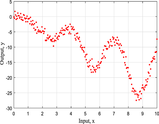
Figure 1. Training data for example 1.

The kernel models are defined as

$\begin{array}{ll}& M_1:k_{\mathit{SE}}={\sigma }^2\text{exp}\left(-\frac{r}{2{\ell }^2}\right)\\ & M_2:k_{\mathit{Ma}}={\sigma }^2\left(1+\frac{\sqrt{5}r}{\ell }+\frac{5r^2}{3{\ell }^2}\right)\text{exp}\left(-\frac{\sqrt{5}r}{\ell }\right)\\ & M_3:k_{\mathit{RQ}}={\sigma }^2{\left(1+\frac{r^2}{2\alpha {\ell }^2}\right)}^{-\alpha }\\ & \text{where}r=∥x-x^{\prime }∥.\end{array}$ (13)

The SE kernel (as stated in the definition of GPs previously) is the most common and default kernel for GPs or even RVMs. As a kernel, it has some nice properties. It is universal, with trivial integration procedure against most functions. It is clear though that each function in its prior mode has an infinite number of derivatives. Furthermore, and more realistically, it has only two parameters, such as the length scale ℓ that controls the length of the “wiggles” in the function, and as a result it cannot extrapolate more than ℓ units away from the data, and the variance σ² that determines the average distance of a function away from its mean, and usually it works just as a scale factor.

The RQ kernel can be seen as adding together SE kernels with different length scales parameter. As a result, in this case, GP priors of this kernel produce functions, which vary smoothly across along different length scales. The parameter α controls the relative weighting of large-scale or small-scale variations. It is very evident that when α → ∞, then the RQ is the same as the SE.

The reason that the Matern kernel is presented here as well is that allows to control the smoothness and includes a large variety of kernels, which can be proven to be very useful for applications because of this flexibility. For the majority of the people who put together a GP regression or classification exercise, they use extensively the SE or RQ kernels. Both these kernels have closed form solutions (integration) and are a quick and easy solution that will probably work well when one is assuming smooth functions when interpolating.

Figure 2 shows the model posterior probabilities over the different populations and the associated tolerance threshold when ABC algorithm is running. One can easily observe that for high tolerance thresholds, there is no strong evidence that a kernel model is more favorable, but between populations 9 and 11, the algorithm gives the trend to favor the simplest, smoothest SE covariance. In a nutshell, the algorithm tries at first to move toward the simplest model, which is the SE one (something that is not so trivial in the next example). As a result, this means that the more complex model is simply penalized. At population 12, the ABC gives a higher evidence to the SE covariance, which remains the simplest one and ends up by finding the true model at population 17 with strong evidence.

FIGURE 2

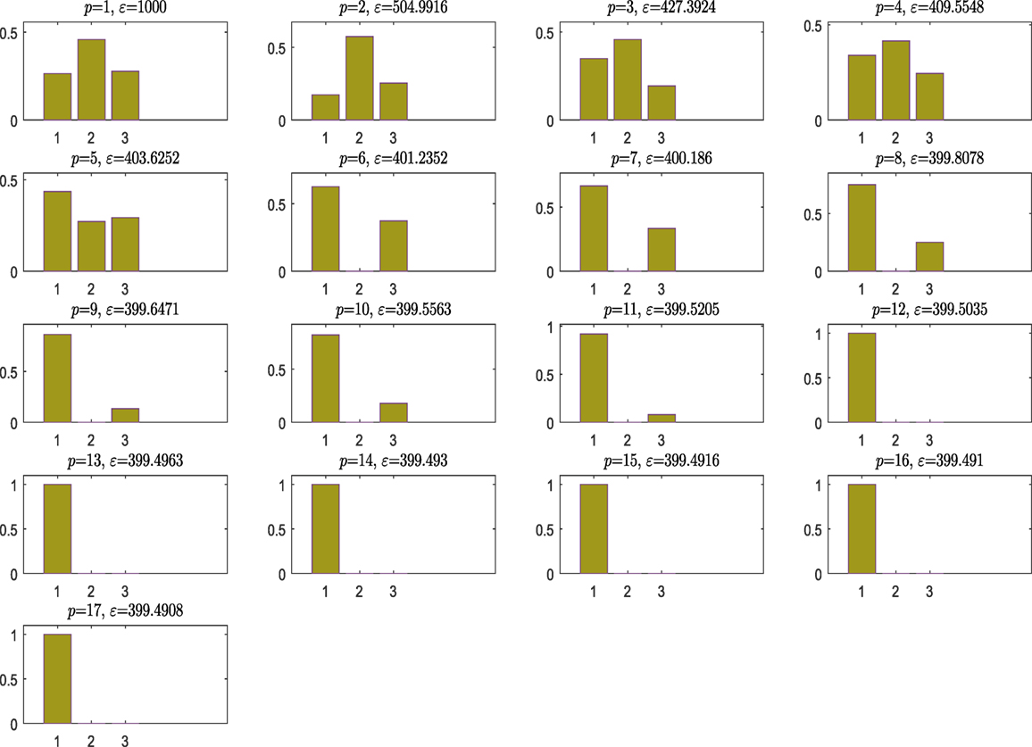
Figure 2. Model posterior probabilities.

From population 12–17, the algorithm refines the model parameter estimates associated to the selected kernel. Figure 3 shows the histograms of the model hyperparameters from the last population.

FIGURE 3

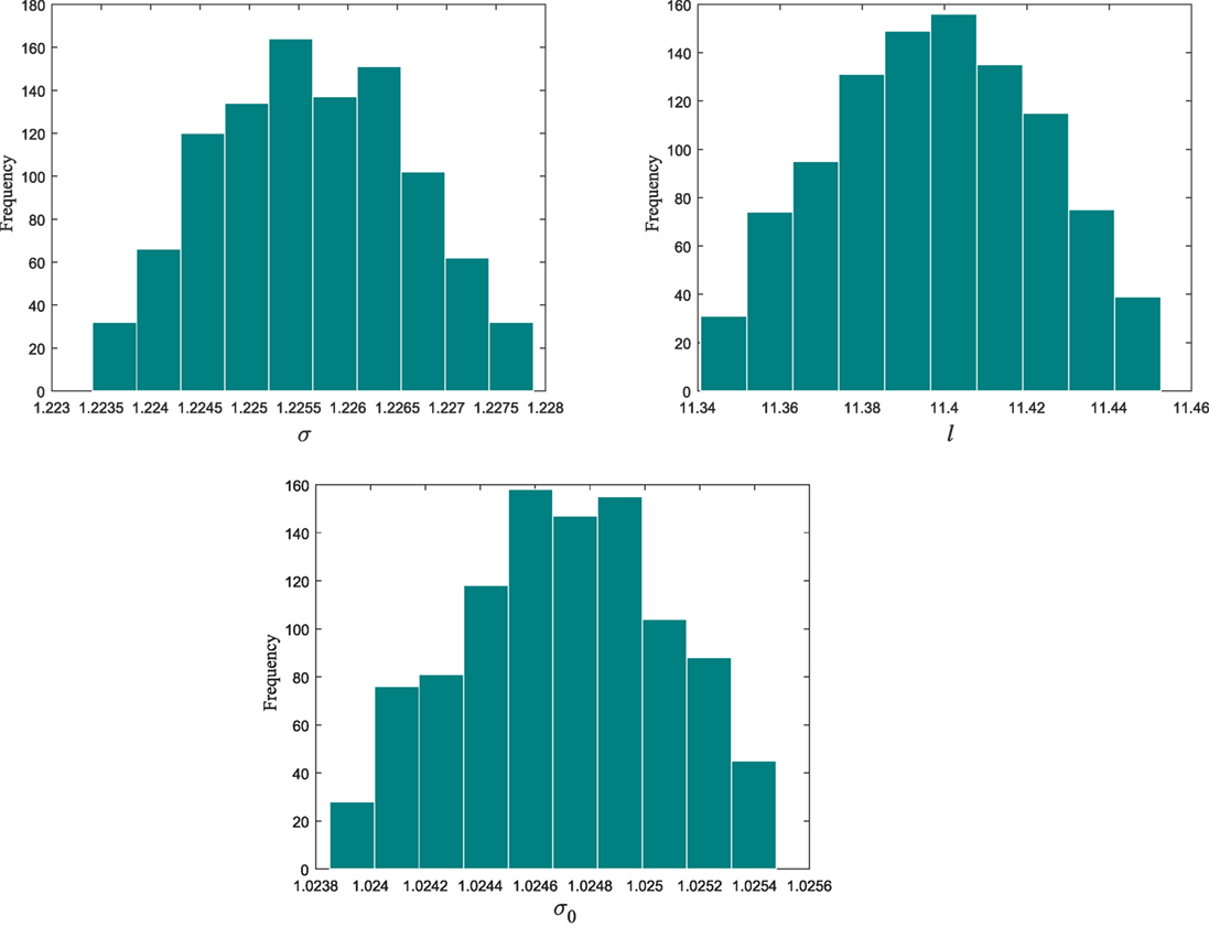
Figure 3. Kernel parameter distributions.

Figures 4–6 show the training data and the model prediction with the 95% confidence interval for all different kernels. One observes a good agreement between the observed and predicted data. In the next real application example, one is able to follow a more interesting and complex behavior on how the ABC algorithm chooses the right kernel model by favoring the simplest model at the beginning but choosing the more complex one at the end.

FIGURE 4

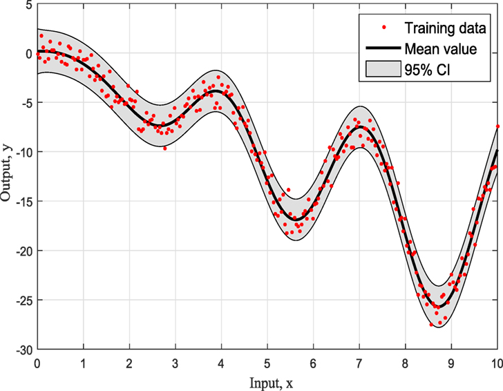
Figure 4. Model 1, SE.

FIGURE 5

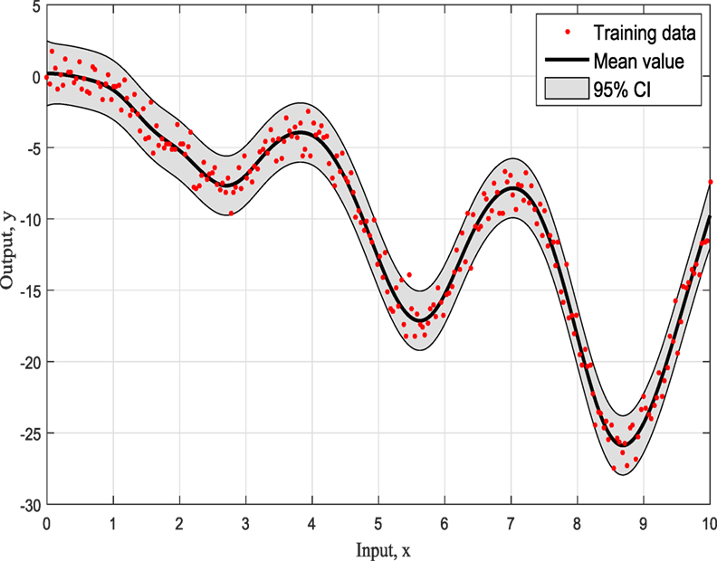
Figure 5. Model 2, MATERN.

FIGURE 6

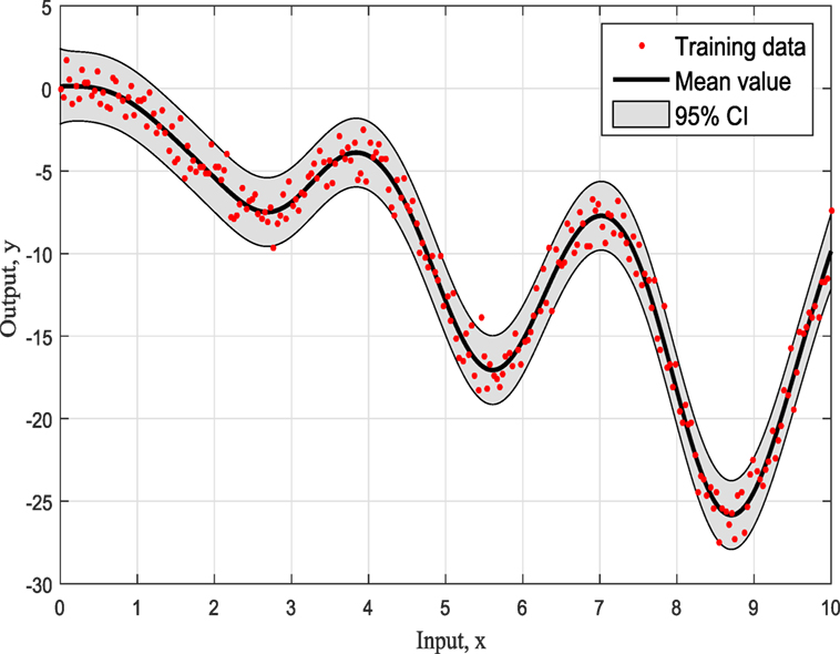
Figure 6. Model 3, RQ.

To summarize so, why it chooses SE kernel against RQ kernel for example. First of all, one has to notice that both of them are giving very similar results in Figures 4 and 5. However, this is the beauty of the methodology followed via ABC-SMC; it scales that both are similar, so there is no need to choose RQ as it is more complicated than SE. If simplicity is good, then keep it as there is no need to add complexity both mathematically and computationally. Another point that it is noticeable is that in Figure 6 where Ma kernel is evaluated there are many “wiggles” and no outliers, but with 95% confidence intervals, one expects a percent of outliers to be present as it happens in Figures 4 and 5.

5. Real Data Application

All three kernels described and mentioned earlier are very useful but if and only if the data is all of the same type with similar feature space. In real applications thought if one wants to perform regression and construct a kernel, then for all different feature/data types, one can multiply kernels together. This is the common standard way to combine kernels together. In simple probabilistic language kernels, multiplication can be considered as an “and” operation. At the same spirit, adding kernels can be considered as an “or” operation.

So the motivation here (as one can do the exact same exercise with different kernels as before) is that the model/data structure one needs are not described by some known kernel (independently of how many different kernels one uses). And for demonstration reasons, the next real data, toy example, is used. One can with different ways to construct kernel combinations with different properties that would allow to include as much high-level structure as possible and check at the same time which of the “modified” models is the best.

For the purposes of this example of composite covariance matrix, two competing models are considered

$\begin{array}{ll}& M_1:k^{\mathit{SE}}+k^{\mathit{PER}}\times k^{\mathit{SE}}+k^{\mathit{RQ}}+k^{\mathit{SE}}\\ & M_2:k^{\mathit{SE}}+k^{\mathit{PER}}\times k^{\mathit{Ma}}+k^{\mathit{Ma}}\end{array}$ (14)

where PER is the periodic kernel, which allows one to model functions that repeat themselves exactly. The period p determines the distance between repetitions of the function, and the length scale is identical to SE kernel. The PER kernel is given by

$k_{\mathit{PER}}={\sigma }^2\text{exp}\left(-\frac{\frac{2{\text{sin}}^2\left(\pi r\right)}{p}}{{\ell }^2}\right).$ (15)

The data that were used here consist of CO₂ concentrations from Mauna Loa observatory, and the reader can find more details in Keeling et al. (1976), Thoning et al. (1989), Etheridge et al. (1996), and Tans (2012) (see Figure 7).

FIGURE 7

Figure 7. Training data for example 2.

Keeling and Whorf (Keeling and Whorf, 2005; Rasmussen and Williams, 2006; Wilson and Adams, 2013) recorded monthly average atmospheric CO₂ concentrations at the Mauna Loa Observatory in Hawaii. The months between around 1960 and 1998 are used for training (see Figure 7), and the remaining months until year 2020 (including GPs extrapolation) are used for testing (see Figure 12).

A very similar dataset was used in Keeling and Whorf (2005), Rasmussen and Williams (2006), and Wilson and Adams (2013) and is often utilized in GPs’ tutorials to demonstrate how GPs are performing as flexible black box modeling tools (even during extrapolation). This data set is great as a toy example as one can notice a long-term rising trend including some seasonal variability and some irregularities. The current work goes toward a fully automated algorithm and investigation for data pattern recognition and robust GP modeling. In all procedures (as before), Gaussian noise is assumed, so that marginalization (or in simple terms integration) over the unknown functions can be performed in a closed form.

M₁ and M₂ in this example are composed of 12 and 9 hyperparameters {θ} (as seen in Figure 9), respectively, and Figure 11 shows the prediction and the 95% according to Rasmussen, while Figure 12 shows the prediction and the 95% confidence bounds by propagating the uncertainty in the hyperparameters.

On running ABC, Figure 8 shows the model posterior probabilities over the different populations and the associated tolerance threshold. One can easily observe that for high tolerance thresholds, there is no strong evidence that either kernel model is more favorable. Between populations 2 and 17, the algorithm gives the trend to favor the simplest covariance. In a nutshell, the algorithm tries at first to converge toward the most simple model, which is the Model Two. This means that the complex model with higher number of parameters (Model One) is penalized. For instance, this is quite obvious at population 9, where the probability associated with Model Two is much higher than Model One. However, by further decreasing the tolerance threshold, it seems that the Model Two is no longer able to give good model prediction with adequate accuracy and in turn, the algorithm moves to favor the more complex Model One. At population 19, the algorithm gives a higher evidence to the Model One. The algorithm ends up by finding the best model at population 23 with strong evidence and eliminates Model Two, which is no longer able to explain the data.

FIGURE 8

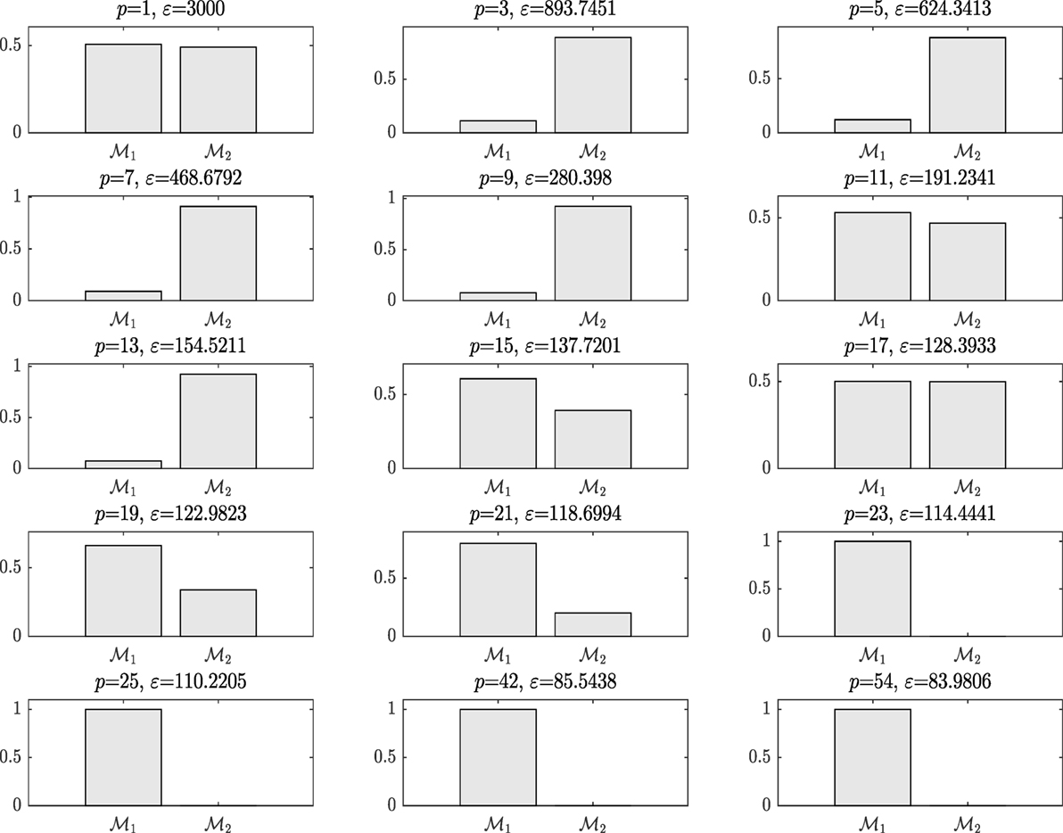
Figure 8. Model posterior probabilities, example 2.

In the subsequent iterations, the algorithm refines the model parameter estimates associated to the best model. Figure 9 shows the histograms of the Model One kernel parameters. By making a comparison between the log-marginal likelihood values obtained with a gradient-based optimizer and ABC-SMC algorithm over the populations, one clearly sees from Figure 10 how the ABC-SMC algorithm converges to a better optimum. This proves the ability of the ABC-SMC algorithm to better explore the input space mainly when one has to deal with high-dimensional problems.

FIGURE 9

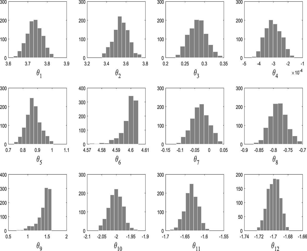
Figure 9. Histograms of the selected model parameters M₁.

FIGURE 10

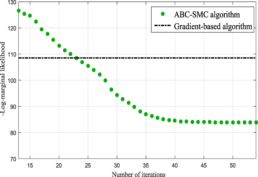
Figure 10. Comparison between the log-marginal likelihood values using gradient-based optimizer and ABC-SMC.

Figures 11 and 12 show the training data and the model prediction with the 95% confidence interval for all different kernels. Figure 11 is obtained according to Rasmussen and Williams (2006), while Figure 12 is obtained by propagating the uncertainty on the hyperparameter estimates, and the kernel was chosen automatically and not by trial and error (important difference). One can see a good agreement between both predictions.

FIGURE 11

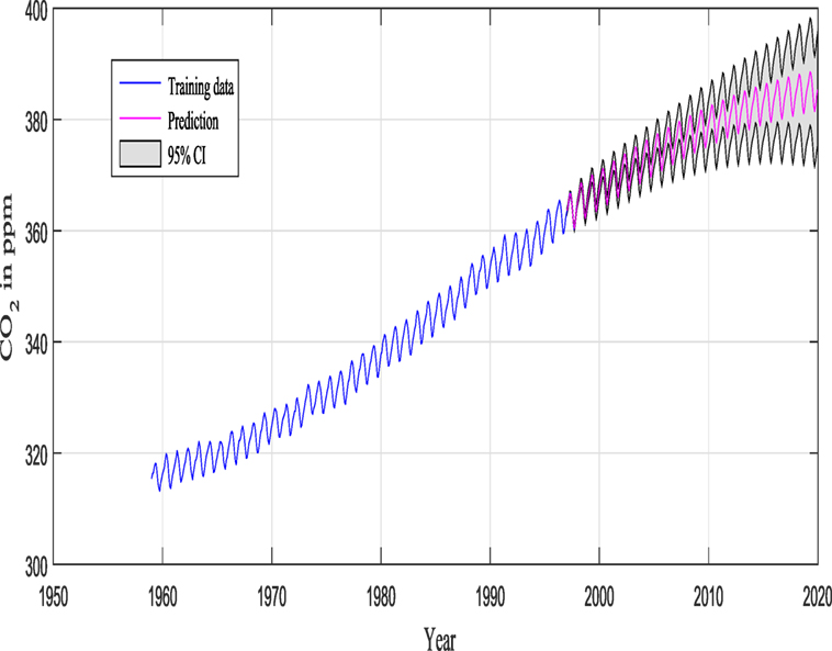
Figure 11. 95% CI obtained according to Rasmussen and Williams.

FIGURE 12

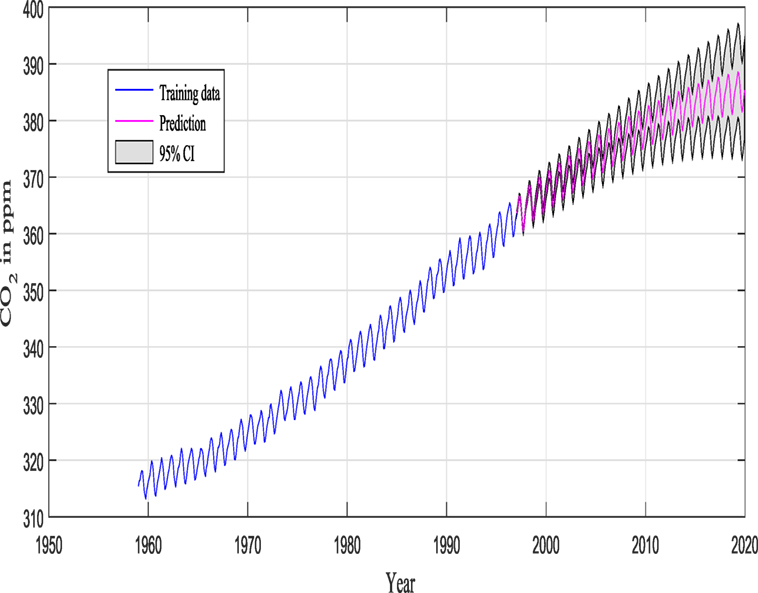
Figure 12. 95% CI obtained from propagating uncertainty in the hyperparameters.

6. Discussion and Conclusion

It is evident from the last example that it was different at the beginning to favor one kernel model against the other. This means that both kernels could be candidates that can explain and fit the data. As the algorithm progresses though, and the threshold tightens, the ABC will jump to the more complex model to understand the trend and the behavior of the data, by forgetting the insufficient properties of the simplest combined kernel. It is clear that the method presented here gives to the end user a systematic and consistent way of choosing kernels for machine learning applications and simultaneously estimating the parameters that accompany them. Given these distributions of the hyperparameters, one can even give confidence intervals that are estimated from the obtained posterior distribution of kernel hyperparameters by generating randomly a large number of samples, simulating the kernel model responses and a pointwise confidence interval can be obtained.

One small comment can now generate a huge discussion that is outside the remit of this paper but can give to the reader food for thought. Why might someone need the uncertainty around the hyperparameters? Are they giving any more information for GP or RVM for example?

The answer is yes and no. It is very evident that kernel selection (or even the mean function) controls all the generalization properties of the algorithm, but as semi- or non-parametric tools like GPs, the uncertainty of the hyperparameters might not add something to the physical mechanism of this Bayesian tool. However, one can argue that they can potentially be used for the evaluation of the training set. GPs or RVMs do not over-fit in the sense of a classical neural network or trapped to local minima as they are closed formed solutions by integrating out the parameters and as a result not having an actual classic error or cost function. But they are “optimized” by giving a specific training set and the uncertainty arising from fitting the best kernel and the best hyperparameters values can be used as “metric” to evaluate if something is wrong with the defined training set and furthermore to check that even different kernel models might struggle to understand the data, which means that the training set is not representative when projected to a validation/test set. Also, if one moves to dynamic models like NARX-GPs, the current work can find not only the best lags number by treating them as different competing models but also a beautiful uncertainty evaluation of choosing specific lags to represent the dynamic regression algorithm.

To summarize, the presented work moves forward to a compact, consistent, and automatic mechanism via Bayesian formulation of the ABC to find an optimal kernel and its hyperparameters simultaneously. As can be seen in example one, the difference between kernels is not significant and this is the reason that the simplest kernel is chosen. In the authors’ opinion, this can generate an argument like a “no free lunch theorem” as for certain types of engineering problems (non-linear systems for example), the computational cost of reaching a solution, averaged over all different models in the same problem, could be simply the same for any “optimized” solution algorithm or kernel model, leaving one with the question is there a best model with best solution that offers a clear “short cut”?

Author Contributions

All authors listed have made a substantial, direct, and intellectual contribution to the work and approved it for publication.

Conflict of Interest Statement

The authors declare that the research was conducted in the absence of any commercial or financial relationships that could be construed as a potential conflict of interest.

The reviewer, LA, and handling editor declared their shared affiliation, and the handling editor states that the process nevertheless met the standards of a fair and objective review.

Funding

This work was supported by the U.K. Engineering and Physical Sciences Research Council (EPSRC) under Grant EP/J016942/1 and Grant EP/K003836/2.

References

Ahn, K., Kim, D., Kim, Y., Park, C., and Kim, I. (2015). Gaussian process model for control of an existing building, 6th International Building Physics Conference, IBPC 2015. Energy Procedia 78, 2136–2141. doi: 10.1016/j.egypro.2015.11.295

CrossRef Full Text | Google Scholar

Akaike, H. (1998). “Information theory and an extension of the maximum likelihood principle,” in Selected Papers of Hirotugu Akaike (Springer), 199–213.

Google Scholar

Au, S.-K., and Beck, J. L. (2001). Estimation of small failure probabilities in high dimensions by subset simulation. Probab. Eng. Mech. 16, 263–277. doi:10.1016/S0266-8920(01)00019-4

CrossRef Full Text | Google Scholar

Barnes, C. P., Silk, D., and Stumpf, M. P. (2011). Bayesian design strategies for synthetic biology. Interface Focus 1, 895–908. doi:10.1098/rsfs.2011.0056

PubMed Abstract | CrossRef Full Text | Google Scholar

Beaumont, M. A., Cornuet, J.-M., Marin, J.-M., and Robert, C. P. (2009). Adaptive approximate Bayesian computation. Biometrika 96, 983–990. doi:10.1093/biomet/asp052

CrossRef Full Text | Google Scholar

Ben Abdessalem, A., Dervilis, N., Wagg, D., and Worden, K. (2016). “Identification of nonlinear dynamical systems using approximate Bayesian computation based on a sequential Monte Carlo sampler,” in Proceedings of ISMA2016 Including USD2016 (Sheffield), 2551–2566.

Google Scholar

Ben Abdessalem, A., Dervilis, N., Wagg, D., and Worden, K. (2017). Model selection and parameter estimation in structural dynamics using approximate Bayesian computation. Mech. Syst. Signal Process. 99, 306–325. doi:10.1016/j.ymssp.2017.06.017

CrossRef Full Text | Google Scholar

Bishop, C. M. (1995). Neural Networks for Pattern Recognition. Oxford University Press.

Google Scholar

Chatzi, E. N., and Smyth, A. W. (2009). The unscented Kalman filter and particle filter methods for nonlinear structural system identification with non-collocated heterogeneous sensing. Struct. Control Health Monit. 16, 99–123. doi:10.1002/stc.290

CrossRef Full Text | Google Scholar

Chatzi, E. N., and Smyth, A. W. (2013). Particle filter scheme with mutation for the estimation of time-invariant parameters in structural health monitoring applications. Struct. Control Health Monit. 20, 1081–1095. doi:10.1002/stc.1520

CrossRef Full Text | Google Scholar

Chiachio, M., Beck, J. L., Chiachio, J., and Rus, G. (2014). Approximate Bayesian computation by subset simulation. SIAM J. Sci. Comput. 36, A1339–A1358. doi:10.1137/130932831

CrossRef Full Text | Google Scholar

Ching, J., Beck, J. L., and Porter, K. A. (2006). Bayesian state and parameter estimation of uncertain dynamical systems. Probab. Eng. Mech. 21, 81–96. doi:10.1016/j.probengmech.2005.08.003

CrossRef Full Text | Google Scholar

Cross, E. (2012). On Structural Health Monitoring in Changing Environmental and Operational Conditions. Dissertation, University of Sheffield.

Google Scholar

Dervilis, N. (2013). A Machine Learning Approach to Structural Health Monitoring with a View towards Wind Turbines. Dissertation, University of Sheffield.

Google Scholar

Dervilis, N., Antoniadou, I., Cross, E. J., and Worden, K. (2015). A non-linear manifold strategy for SHM approaches. Strain 51, 324–331. doi:10.1111/str.12143

CrossRef Full Text | Google Scholar

Dervilis, N., Shi, K., Worden, K., and Cross, E. J. (2016). Exploring environmental and operational variations in SHM data using heteroscedastic Gaussian processes. Dyn. Civ. Struct. 2, 145–153. doi:10.1007/978-3-319-29751-4_15

CrossRef Full Text | Google Scholar

Doucet, A., De Freitas, N., and Gordon, N. (2001). “An introduction to sequential Monte Carlo methods,” in Sequential Monte Carlo Methods in Practice (Springer), 3–14.

Google Scholar

Doucet, A., Godsill, S., and Andrieu, C. (2000). On sequential Monte Carlo sampling methods for Bayesian filtering. Stat. Comput. 10, 197–208. doi:10.1023/A:1008935410038

CrossRef Full Text | Google Scholar

Etheridge, D. M., Steele, L., Langenfelds, R., Francey, R., Barnola, J.-M., and Morgan, V. (1996). Natural and anthropogenic changes in atmospheric CO2 over the last 1000 years from air in Antarctic ice and firn. J. Geophys. Res. Atmos. 101, 4115–4128. doi:10.1029/95JD03410

CrossRef Full Text | Google Scholar

Filippi, S., Barnes, C. P., Cornebise, J., and Stumpf, M. P. (2013). On optimality of kernels for approximate Bayesian computation using sequential Monte Carlo. Stat. Appl. Genet. Mol. Biol. 12, 87–107. doi:10.1515/sagmb-2012-0069

PubMed Abstract | CrossRef Full Text | Google Scholar

Green, P. J. (1995). Reversible jump Markov chain Monte Carlo computation and Bayesian model determination. Biometrika 82, 711–732. doi:10.1093/biomet/82.4.711

CrossRef Full Text | Google Scholar

Gretton, A., Borgwardt, K. M., Rasch, M., Schölkopf, B., and Smola, A. J. (2007). “A kernel approach to comparing distributions,” in Proceedings of the National Conference on Artificial Intelligence, 1999, Vol. 22 (Menlo Park, CA; Cambridge, MA; London: AAAI Press; MIT Press), 1637.

Google Scholar

Hensman, J., Fusi, N., and Lawrence, N. D. (2013). Gaussian Processes for Big Data. arXiv preprint arXiv:1309.6835.

Google Scholar

Keeling, C., and Whorf, T. (2005). “Atmospheric carbon dioxide record from Mauna Loa,” in Trends: A Compendium of Data on Global Change (Oak Ridge, TN: Carbon Dioxide Information Analysis Center, Oak Ridge National Laboratory).

Google Scholar

Keeling, C. D., Bacastow, R. B., Bainbridge, A. E., Ekdahl, C. A. Jr., Guenther, P. R., Waterman, L. S., et al. (1976). Atmospheric carbon dioxide variations at Mauna Loa Observatory, Hawaii. Tellus 28, 538–551. doi:10.3402/tellusa.v28i6.11323

CrossRef Full Text | Google Scholar

Kullback, S. (1997). Information Theory and Statistics. Courier Corporation.

Google Scholar

Lawrence, N. D. (2003). “Gaussian process latent variable models for visualisation of high dimensional data,” in Nips, Vol. 2, 5.

Google Scholar

Marjoram, P., Molitor, J., Plagnol, V., and Tavaré, S. (2003). Markov chain Monte Carlo without likelihoods. Proc. Natl. Acad. Sci. U.S.A. 100, 15324–15328. doi:10.1073/pnas.0306899100

PubMed Abstract | CrossRef Full Text | Google Scholar

Nabney, I. (2002). NETLAB: Algorithms for Pattern Recognition. Springer Science & Business Media.

Google Scholar

Neath, A. A., and Cavanaugh, J. E. (2012). The Bayesian information criterion: background, derivation, and applications. Wiley Interdiscip. Rev. Comput. Stat. 4, 199–203. doi:10.1002/wics.199

CrossRef Full Text | Google Scholar

Rasmussen, C. E., and Williams, C. K. I. (2006). Gaussian Processes for Machine Learning.

Google Scholar

Schwarz, G., et al. (1978). Estimating the dimension of a model. Ann. Stat. 6, 461–464. doi:10.1214/aos/1176344136

CrossRef Full Text | Google Scholar

Skilling, J. (2006). Nested sampling for general Bayesian computation. Bayesian Anal. 1, 833–859. doi:10.1214/06-BA127

CrossRef Full Text | Google Scholar

Su, G., Peng, L., and Hu, L. (2017). A Gaussian process-based dynamic surrogate model for complex engineering structural reliability analysis. Struct. Saf. 68, 97–109. doi:10.1016/j.strusafe.2017.06.003

CrossRef Full Text | Google Scholar

Tans, D. P. (2012). Noaa/esrl (http://www.esrl.noaa.gov/gmd/ccgg/trends/) and Dr. Ralph Keeling. Scripps Institution of Oceanography (http://scrippsco2.ucsd.edu/).

Google Scholar

Thoning, K. W., Tans, P. P., and Komhyr, W. D. (1989). Atmospheric carbon dioxide at Mauna Loa Observatory: 2. Analysis of the NOAA GMCC data, 1974–1985. J. Geophys. Res. Atmos. 94, 8549–8565. doi:10.1029/JD094iD06p08549

CrossRef Full Text | Google Scholar

Toni, T., and Stumpf, M. P. (2010). Simulation-based model selection for dynamical systems in systems and population biology. Bioinformatics 26, 104–110. doi:10.1093/bioinformatics/btp619

PubMed Abstract | CrossRef Full Text | Google Scholar

Toni, T., Welch, D., Strelkowa, N., Ipsen, A., and Stumpf, M. P. (2009). Approximate Bayesian computation scheme for parameter inference and model selection in dynamical systems. J. R. Soc. Interface 6, 187–202. doi:10.1098/rsif.2008.0172

PubMed Abstract | CrossRef Full Text | Google Scholar

Turner, B. M., and Van Zandt, T. (2012). A tutorial on approximate Bayesian computation. J. Math. Psychol. 56, 69–85. doi:10.1016/j.jmp.2012.06.004

CrossRef Full Text | Google Scholar

Wan, H., Mao, Z., Todd, M., and Ren, W. (2014). Analytical uncertainty quantification for modal frequencies with structural parameter uncertainty using a Gaussian process metamodel. Eng. Struct. 75, 577–589. doi:10.1016/j.engstruct.2014.06.028

CrossRef Full Text | Google Scholar

Wan, H., and Ren, W. (2015). A residual-based Gaussian process model framework for finite element model updating. Comput. Struct. 156, 149–159. doi:10.1016/j.compstruc.2015.05.003

CrossRef Full Text | Google Scholar

Wilson, A., and Adams, R. (2013). “Gaussian process kernels for pattern discovery and extrapolation,” in Proceedings of the 30th International Conference on Machine Learning (ICML-13), 1067–1075.

Google Scholar

Worden, K., and Cross, E. J. (2018). On switching response surface models, with applications to the structural health monitoring of bridges. Mech. Syst. Signal Process. 98, 139–156. doi:10.1016/j.ymssp.2017.04.022

CrossRef Full Text | Google Scholar

Worden, K., Staszewski, W. J., and Hensman, J. J. (2011). Natural computing for mechanical systems research: a tutorial overview. Mech. Syst. Signal Process. 25, 4–111. doi:10.1016/j.ymssp.2010.07.013

CrossRef Full Text | Google Scholar