Critical Response of Single-Degree-of-Freedom Damped Bilinear Hysteretic System under Double Impulse As Substitute for Near-Fault Ground Motion

Introduction

Earthquake ground motions have been classified based on their characteristics (Abrahamson et al., 1998). This stream is being accelerated as many useful data from recent earthquakes are accumulated. One is a near-fault ground motion and another one is a long-period and long-duration ground motion mostly characterized as a far-fault motion (see Takewaki et al., 2011). It is well known that earthquake ground motions at ground surface are influenced greatly by the surface-soil properties. For this reason, the surface-soil types (soil and rock) are other factors for classification together with fault mechanisms. The effects of near-fault ground motions on structural inelastic responses have been investigated from various viewpoints (for example, Bertero et al., 1978; Hall et al., 1995; Sasani and Bertero, 2000; Mavroeidis and Papageorgiou, 2003; Alavi and Krawinkler, 2004; Makris and Black, 2004; Mavroeidis et al., 2004; Kalkan and Kunnath, 2006; Khaloo et al., 2015). The special terminologies of fling step (parallel to the fault plane) and forward directivity (normal to the fault plane) are often used recently for designating such near-fault ground motions. Many earthquake structural engineers pay special attention to Northridge earthquake in 1994, Hyogoken-Nanbu (Kobe) earthquake in 1995, Chi-Chi (Taiwan) earthquake in 1999, and Kumamoto earthquake in 2016.

The main parts of fling-step and forward-directivity motions have been characterized by using two or three half-cycle sine waves (see Figure 1). Most engineers investigated mainly the elastic response in the past works on the near-fault ground motions. This is because there are many parameters (e.g., predominant period, duration and amplitude of pulse, change of equivalent natural frequency for the increased input level, and ratio of pulse frequency to structure natural frequency) and even the numerical parametric analysis is extremely complicated for elastic–plastic response.

FIGURE 1

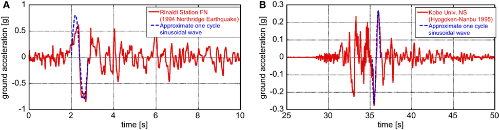
Figure 1. Simplification of main part of actual pulse-type ground motion into one-cycle sine wave: (A) fault-normal component at Rinaldi station (Northridge earthquake 1994), (B) NS component (almost fault-normal) at Kobe University [Hyogoken-Nanbu (Kobe) earthquake 1995] (Kojima and Takewaki, 2016).

To respond to such complex issue, an innovative approach using the double impulse as expressed in Figure 2A was developed by Kojima and Takewaki (2015a). The double impulse substitutes approximately for the main part of the fling-step near-fault ground motion as a one-cycle sine wave, and the explicit maximum elastic–plastic response was obtained in a structure under the “critical double impulse.” The concept of “critical input” is based on the critical excitation method in which it is aimed at finding the worst input (see Drenick, 1970; Takewaki, 2007). Because only the free vibration emerges under such double impulse, the energy balance approach for the kinetic energy, hysteretic and strain energies, and damping energy leads to such explicit expression. It was also shown that, depending on the input level of the double impulse, the maximum inelastic deformation can occur either after the first or second impulse. The accuracy and validity of the proposed explicit expression were made clear by comparing such expressions with the time-history response analysis results under the equivalent one-cycle sine wave, a representative of the main part of the fling-step near-fault ground motion. The magnitude of the double impulse was adjusted based on the criterion that the maximum Fourier amplitude is equivalent to that of the one-cycle sine wave. By introducing the triple impulse, the methodology for the fling-step motion was applied successfully to a more realistic forward-directivity motion by Kojima and Takewaki (2015b) (see Figure 2B).

FIGURE 2

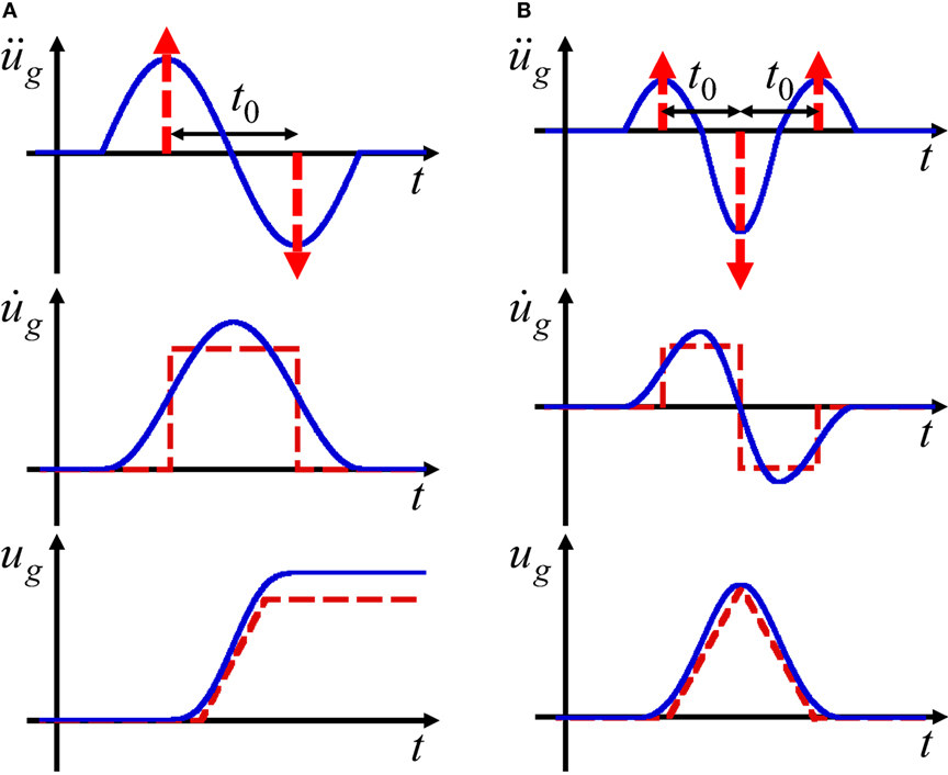
Figure 2. Main part of near-fault ground motion, (A) fling-step input and double impulse, (B) forward-directivity input and triple impulse (Kojima and Takewaki, 2015a).

The analytical expressions of the dynamic elastic–plastic response were obtained only for the harmonic steady-state response and the transient response to a sinusoidal wave (Caughey, 1960a,b, Roberts and Spanos, 1990, Liu, 2000). It should be reminded that the forced input by the sinusoidal wave caused a complexity in deriving simple expressions on responses. It may be natural and interesting to recall that, if a near-fault ground motion can be modeled into a double impulse, the maximum elastic–plastic response can be derived in terms of continuation of free vibrations by taking advantage of an energy balance approach without the direct solution of the equation of motion (Kojima and Takewaki, 2015a).

In the historical context of earthquake-resistant design in the last century, the resonance was a key subject in the damage analysis of structures. For a specified input level, the resonant equivalent frequency has to be analyzed generally by changing the input frequency of a sine wave in a parametric manner (Caughey, 1960a,b, Iwan, 1961, 1965a,b, Roberts and Spanos, 1990, Liu, 2000). The double impulse enables such computation without repetition. In the double impulse input, the resonance can be captured by taking advantage of an energy balance law and the timing of the second impulse can be characterized as the time with zero restoring force after the first impulse. The peak elastic–plastic response after the first impulse can be derived by equating the initial kinetic energy given by the impulse to the sum of hysteretic energy, elastic strain energy, and the damping energy in the damped system (Kojima et al., 2017).

In this paper, the double impulse is used as a good substitute for a one-cycle sine wave which expresses the main part of the near-fault ground motion and an explicit expression is derived on the maximum elastic–plastic response of a damped single-degree-of-freedom (SDOF) structure with bilinear hysteresis under the “critical double impulse input.” A damped bilinear hysteretic SDOF system is introduced in Section “Damped Bilinear Hysteretic SDOF System.” The closed-form expressions are derived in Section “Closed-Form Expression of Maximum Elastic–Plastic Response under Critical Double Impulse” on the maximum elastic–plastic responses under the critical double impulse by using the energy balance approach and the quadratic function approximation of the damping force–deformation relation of the dashpot (Kojima et al., 2017). The combination of damping and bilinear hysteresis is a novel point in this paper. Depending on the input level, three cases are defined. CASE 1 is the case where the model remains elastic even after the second impulse and CASE 2 is the case where the model goes into the plastic range only after the second impulse. Furthermore CASE 3 is the case where the model goes into the plastic range even after the first impulse. In CASE 3, there are two more cases, i.e., CASE 3-1 where the zero-restoring-force timing after the first impulse exists in the unloading stage and CASE 3-2 where the zero-restoring-force timing after the first impulse exists in the reloading stage after the unloading stage. The critical time interval is obtained in Section “Critical Impulse Timing” by regarding the zero-restoring-force timing as the critical timing. The accuracy of the proposed expression on the maximum response is investigated by comparing with the results by time-history response analysis of the SDOF damped bilinear hysteresis system under the double impulse in Section “Accuracy Check of the Proposed Expression under the Double Impulse through the Comparison with the Time-History Response Analysis under the Double Impulse and the Corresponding One-Cycle Sinusoidal Wave.” The accuracy of using the double impulse is also checked in Section “Accuracy Check of the Proposed Expression under the Double Impulse through the Comparison with the Time-History Response Analysis under the Double Impulse and the Corresponding One-Cycle Sinusoidal Wave” by comparing with the response to the equivalent one-cycle sine wave. The proof of the critical impulse timing obtained in Section “Critical Impulse Timing” and its interpretation as the zero-restoring-force timing are investigated in Section “Proof of Critical Timing.” The accuracy check of the response under the critical double impulse is conducted through the comparison with the time-history response to the equivalent one-cycle sine wave in Section “Accuracy Check of the Response under the Critical Double Impulse through the Comparison with the Time-History Response under the Corresponding One-Cycle Sinusoidal Wave.” The application to actual ground motions is shown in Section “Application of Proposed Expression on Critical Response to Recorded Near-Fault Ground Motion.” The conclusions are summarized in Section Conclusion.

Damped Bilinear Hysteretic SDOF System

Consider a damped bilinear hysteretic SDOF system of mass m, initial stiffness k and damping coefficient c subjected to the double impulse ${ü}_g\left(t\right)=\mathit{V\delta }\left(t\right)-\mathit{V\delta }\left(t-t_0\right)$ of ground acceleration as shown in Figure 3. V is the prescribed initial velocity (also the velocity amplitude of the second impulse) and t₀ is the time interval between two impulses which is regarded as a variable in finding the critical double impulse. The ratio of the post-yield stiffness to the initial one is designated by α. In this paper α > 0. The yield deformation and force are expressed by d_y and f_y. Let ${\mathrm{\omega }}_1=\sqrt{k/m}$, $T_1=\mathrm{2\pi }/{\mathrm{\omega }}_1$, ${\mathrm{\omega }}_1^{\prime }=\sqrt{1-h^2}{\mathrm{\omega }}_1$, $T_1^{\prime }=\mathrm{2\pi }/{\mathrm{\omega }}_1^{\prime }$, h, u, and f denote the undamped natural circular frequency, the undamped natural period, the damped natural circular frequency, the damped natural period, the damping ratio, the displacement of the mass relative to the ground (deformation of the system) and the restoring force in the model, respectively. The time derivative is designated by an over-dot. In Section “Closed-Form Expression of Maximum Elastic–Plastic Response under Critical Double Impulse,” these parameters will be dealt with in normalized forms to derive the essential relationship between the input parameters and the elastic–plastic response. Let V_y(=ω₁d_y) denote the velocity amplitude of the double impulse which causes exactly the yield deformation after the first impulse. This parameter is a parameter related to the strength of the SDOF system. The parameter V_y is a normalization parameter for the input velocity level and the ratio V/V_y is called the input velocity level. However, numerical investigations will be made in Sections “Accuracy Check of the Proposed Expression under the Double Impulse through the Comparison with the Time-History Response Analysis under the Double Impulse and the Corresponding One-Cycle Sinusoidal Wave,” “Proof of Critical Timing,” and “Accuracy Check of the Response under the Critical Double Impulse through the Comparison with the Time-History Response under the Corresponding One-Cycle Sinusoidal Wave” to demonstrate an example of actual parameters.

FIGURE 3

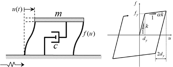
Figure 3. Damped single-degree-of-freedom model and its bilinear hysteretic restoring-force characteristic.

Closed-Form Expression of Maximum Elastic–Plastic Response Under Critical Double Impulse

In the previous related works on energy-based approach (Kojima and Takewaki, 2015a,b,c), some explicit expressions have been derived in the critical response of an SDOF elastic–perfectly plastic system under the double, triple and multi impulses. An explicit expression on the peak deformation of an SDOF bilinear hysteretic system under the double impulse has also been obtained (Kojima and Takewaki, 2016). In contrast to these previous papers, an explicit form of the peak deformation of an SDOF damped bilinear hysteretic system under the critical double impulse is obtained here. The combination of damping and bilinear hysteresis is a novel point in this paper.

The response just after each impulse can be described by the sudden change of velocity of the structural mass by V and only free vibration exists after each impulse. Because the elastic–plastic response of the SDOF damped bilinear hysteretic system under the double impulse can be described by the direct continuation of free vibrations with different initial velocities and deformations, the maximum deformation can be derived by a sophisticated energy approach without the direct solution of the equation of motion. The kinetic energy introduced at each impulse is transformed into the combination of the hysteretic energy, the elastic strain energy and the viscously damped energy. It should be remarked that the critical timing of the second impulse corresponds to the zero-restoring-force timing after the first impulse and a kinetic energy alone exists at this timing as mechanical energies. By using this rule on energy balance, the expression on the peak deformation can be obtained in a simple way. In the previous work (Kojima and Takewaki, 2015a), the explicit form of the maximum deformation and the critical timing of the elastic–perfectly plastic SDOF system under the critical double impulse have been obtained. In this section, the explicit expressions of the peak response are derived by using the energy approach and the critical timing is obtained. Since it seems difficult to derive an exact expression on the damping force with respect to deformation, a quadratic function approximation is introduced for the damping force–deformation relation to evaluate the viscously damped energy (the work done by the damping force). Using this approximation, the viscously damped energy can be evaluated by using the damping force at the acting point of the first or second impulse and the maximum deformation (Kojima et al., 2017). In Sections “Closed-Form Expression of Maximum Elastic–Plastic Response under Critical Double Impulse” and “Accuracy Check of the Proposed Expression under the Double Impulse through the Comparison with the Time-History Response Analysis under the Double Impulse and the Corresponding One-Cycle Sinusoidal Wave,” this approximation is used to obtain the velocity at the point of the re-yielding initiation.

The maximum response under the critical double impulse can be divided into three cases depending on the plastic deformation level. Each case will be explained in the following.

CASE 1: Elastic Response Even after Second Impulse

First, consider CASE 1 where the structure exhibits elastic response even after the second impulse. Figure 4 shows the evaluation process of the peak deformation u_max1 after the first impulse and the peak deformation u_max2 after the second impulse for the elastic case (CASE 1) (see Figure 4A for restoring force). Although an approximate and exact solution for the elastic response of the system with viscous damping was obtained in the previous paper (Kojima et al., 2017), the derivation of the approximate expression of the peak deformation is shown here for better explanation of subsequent cases. It uses approximation in terms of the quadratic function for the damping force–deformation relation. The expression is a good approximation of the exact solution.

FIGURE 4

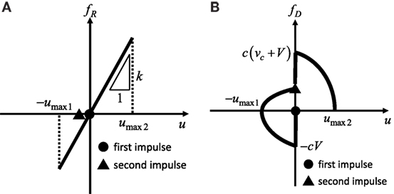
Figure 4. Restoring force and damping force with respect to deformation in CASE 1 [V/V_y ≤ (V/V_y)_{CASE 1}], (A) restoring force–deformation relation, (B) quadratic approximation of damping force–deformation relation.

By using the quadratic function approximation for the damping force–deformation relation, the work done by the damping force f_D after the first impulse can be evaluated. In this process, let us approximate the damping force–deformation relation after the first impulse by a quadratic function with vertex (u, f_D) = (−u_max1, 0) and passing through the point (u, f_D) = (0, −cV), as shown in Figure 4B. The damping force f_D can be obtained as follows:

$f_D=-\mathit{cV}\sqrt{1+\left(u/u_{\text{max}1}\right)}.$ (1)

The work done by the damping force on the corresponding deformation can be obtained by integrating Eq. 1 from u = 0 to u = − u_max1,

${\int }_0^{-u_{\text{max}1}}{f}_D\mathit{du}={\int }_0^{-u_{\text{max}1}}\left\{-\mathit{cV}\sqrt{1+\left(u/u_{\text{max}1}\right)}\right\}\mathit{du}=\left(2/3\right)\mathit{cV}{u}_{\text{max}1}.$ (2)

By using Eq. 2, the energy balance law at the time of the first impulse and the time attaining the maximum deformation leads to

$0.5m{V}^2=0.5k{u_{\text{max}1}}^2+\left(2/3\right)\mathit{cV}{u}_{\text{max}1}.$ (3)

From Eq. 3, u_max1 can be obtained as

$u_{\text{max}1}/d_y=\left\{-\left(4/3\right)h+\sqrt{\left(16/9\right)h^2+1}\right\}\left(V/V_y\right),$ (4)

where h is the damping ratio. In a similar manner, u_max2 can be obtained. The velocity v_c at the zero-restoring-force timing can be derived by using the critical time interval $t_0^c=T_1^{\prime }/2$ ($T_1^{\prime }$: damped natural period) and the velocity response after the first impulse. The critical time interval $t_0^c=T_1^{\prime }/2$ has been obtained for the elastic damped SDOF system in the previous paper (Kojima et al., 2017). The velocity response after the first impulse can be obtained as follows:

$\dot{u}\left(t\right)=-V{\mathrm{e}}^{-h{\mathrm{\omega }}_{1}t}\left\{-\left(h/\sqrt{1-h^2}\right)\text{sin}\left({\mathrm{\omega }}_1^{\prime }t\right)+\cos \left({\mathrm{\omega }}_1^{\prime }t\right)\right\},$ (5)

v_c can be obtained by substituting $t=t_0^c=T_1^{\prime }/2$ into Eq. 5

$v_c=V\text{exp}\left(-\mathrm{\pi }h/\sqrt{1-h^2}\right).$ (6)

The work done by the damping force on the corresponding deformation can be derived by using the quadratic function approximation. It may be reasonable to approximate the damping force–deformation relation after the second impulse by a quadratic function with vertex (u, f_D) = (u_max2, 0) and passing through the point (u, f_D) = (0, c(v_c + V)), as shown in Figure 4B. The damping force f_D can be obtained as follows:

$f_D=c\left(v_c+V\right)\sqrt{1-\left(u/u_{\text{max}2}\right)}.$ (7)

The work done by the damping force on the corresponding deformation after the second impulse can be derived by integrating Eq. 7 from u = 0 to u = u_max2,

${\int }_0^{u_{\text{max}2}}{f}_D\mathit{du}={\int }_0^{u_{\text{max}2}}\left\{c\left(v_c+V\right)\sqrt{1-\left(u/u_{\text{max}2}\right)}\right\}\mathit{du}=\left(2/3\right)c\left(v_c+V\right)u_{\text{max}2}.$ (8)

By using Eq. 8, the energy balance law at the time of the second impulse and the time attaining the maximum deformation leads to

$0.5m{\left(v_c+V\right)}^2=0.5k{u_{\text{max}2}}^2+\left(2/3\right)c\left(v_c+V\right)u_{\text{max}2}.$ (9)

From Eqs 6 and 9, u_max2 can be obtained as

$u_{\text{max}2}/d_y=\left(1+{\mathrm{e}}^{-\mathrm{\pi }h/\sqrt{1-h^2}}\right)\left\{-\left(4/3\right)h+\sqrt{\left(16/9\right)h^2+1}\right\}\left(V/V_y\right).$ (10)

The boundary input velocity level (V/V_y)_{CASE 1} between CASE 1 and CASE 2 in the caption of Figure 4 will be derived in the next section.

CASE 2: Plastic Deformation Only after the Second Impulse

Second, consider CASE 2, where the system goes into the yielding stage only after the second impulse. Figure 5 presents the evaluation process of the maximum deformation u_max1 after the first impulse and the maximum deformation u_max2 after the second impulse in CASE 2. When the maximum deformation u_max2 after the second impulse is beyond the yield deformation d_y for the first time, the system goes into the plastic range after the second impulse. This boundary input velocity level (V/V_y)_{CASE 1} between CASE 1 and CASE 2 can be provided from Eq. 10 and u_max2 = d_y,

${\left(V/V_y\right)}_{\text{CASE 1}}={\left(1+{\text{e}}^{-\mathrm{\pi }h/\sqrt{1-h^2}}\right)}^{-1}\left\{\left(4/3\right)h+\sqrt{\left(16/9\right)h^2+1}\right\}.$ (11)

FIGURE 5

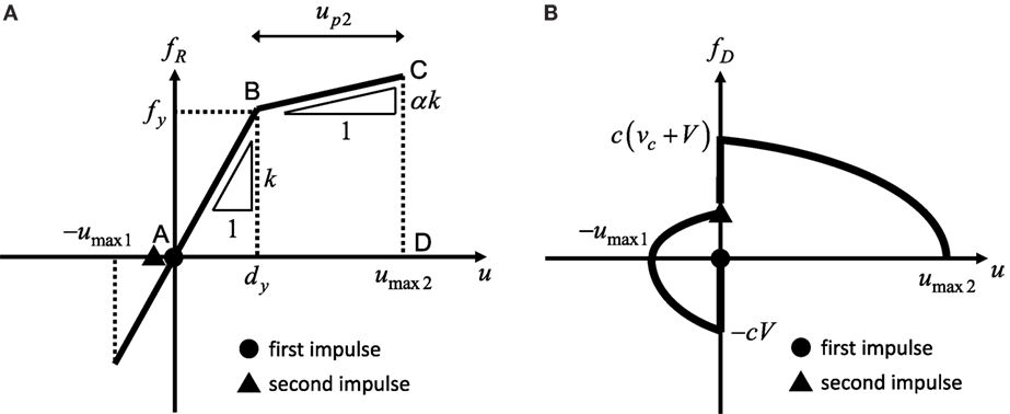
Figure 5. Restoring force and damping force with respect to deformation in CASE 2 [(V/V_y)_{CASE 1} ≤ V/V_y ≤ (V/V_y)_{CASE 2}], (A) restoring force–deformation relation, (B) quadratic approximation of damping force–deformation relation.

Because the maximum deformation just after the first impulse remains in the elastic range, u_max1 in CASE 2 is also given by Eq. 4. The maximum deformation u_max2 in CASE 2 is derived in this section. By using the quadratic function approximation as shown in Figure 5B, the work done by the damping force in CASE 2 can be evaluated. As in CASE 1, the velocity v_c in CASE 2 can be given by Eq. 6 because the response is elastic just after the first impulse. As in CASE 1, by using the quadratic function approximation, the work done by the damping force on the corresponding deformation after the second impulse in CASE 2 can be expressed by Eq. 8. By using Eq. 8, the energy balance law at the time of the second impulse and the time attaining the maximum deformation leads to

$0.5m{\left(v_c+V\right)}^2=\left(\text{area of ABCD}\right)+\left(2/3\right)c\left(v_c+V\right)u_{\text{max}2}.$ (12)

The expression of (area of ABCD) in Eq. 12 indicates the area of the quadrilateral ABCD in Figure 5A. From Eqs 6 and 12, u_max2 can be obtained as

$\begin{array}{l}\frac{u_{\text{max}2}}{d_y}=1-\frac{1}{\mathrm{\alpha }}\left\{1+\frac{4h}{3}\left(1+{\mathrm{e}}^{-\mathrm{\pi }h/\sqrt{1-h^2}}\right)\left(\frac{V}{V_y}\right)\right\}\hfill \\ +\frac{1}{\mathrm{\alpha }}\sqrt{{\left\{1+\frac{4h}{3}\left(1+{\mathrm{e}}^{-\mathrm{\pi }h/\sqrt{1-h^2}}\right)\left(\frac{V}{V_y}\right)\right\}}^2-\mathrm{\alpha }\left\{1+\frac{8h}{3}\left(1+{\mathrm{e}}^{-\mathrm{\pi }h/\sqrt{1-h^2}}\right)\left(\frac{V}{V_y}\right)-{\left(1+{\mathrm{e}}^{-\mathrm{\pi }h/\sqrt{1-h^2}}\right)}^2{\left(\frac{V}{V_y}\right)}^2\right\}}.\hfill \end{array}$ (13)

The boundary input velocity level (V/V_y)_{CASE 2} between CASE 2 and CASE 3 in the caption of Figure 5 will be derived in the next section.

CASE 3-1: Plastic Deformation Even after the First Impulse (Second Impulse in Unloading Process)

Finally, consider CASE 3, where the system enters the yielding stage, even after the first impulse. CASE 3 can be classified into CASE 3-1 and CASE 3-2 depending on the input velocity level. In this section, the closed-form solution for the maximum deformation for CASE 3-1 is derived. In CASE 3-1, the second impulse acts at the zero-restoring-force timing in the unloading process. On the other hand, in CASE 3-2, the second impulse acts at the zero-restoring-force timing in the reloading process (second stiffness range). Figure 6 shows the evaluation process of the maximum deformation u_max1 after the first impulse and the maximum deformation u_max2 after the second impulse in CASE 3-1 and CASE 3-2. When the maximum deformation u_max1 after the first impulse is beyond the yield deformation d_y, the system goes into the plastic range after the first impulse. This boundary input velocity level (V/V_y)_{CASE 2} between CASE 2 and CASE 3-1 can be derived as follows from Eq. 4 and u_max1 = d_y,

${\left(V/V_y\right)}_{\text{CASE 2}}=\left(4/3\right)h+\sqrt{\left(16/9\right)h^2+1}.$ (14)

FIGURE 6

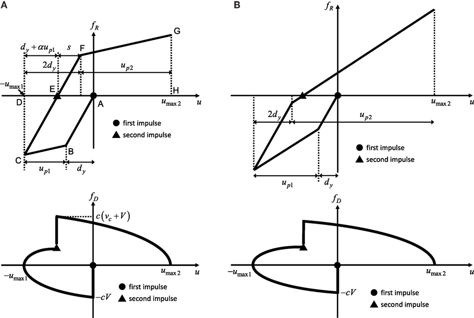
Figure 6. Restoring force–deformation relation and approximate damping force–deformation relation. (A) CASE 3-1: (V/V_y)_{CASE 2} ≤ V/V_y ≤ (V/V_y)_{CASE 3}, (B) CASE 3-2: (V/V_y)_{CASE 3} ≤ V/V_y.

The maximum deformation u_max1 after the first impulse is derived next. The work done by the damping force after the first impulse in CASE 3-1 has been derived, as expressed by Eq. 2, by using the quadratic function approximation. This approximation was also made in CASE 1. By using Eq. 2, the energy balance law at the time of the first impulse and the time attaining the maximum deformation leads to

$0.5m{V}^2=\left(\text{area of ABCD}\right)+\left(2/3\right)\mathit{cV}{u}_{\text{max}1}.$ (15)

The expression of (area of ABCD) in Eq. 15 indicates the area of the quadrilateral ABCD in Figure 6A. From Eq. 15, u_max1 can be obtained as

$\frac{u_{\text{max}1}}{d_y}=1+\frac{1}{\mathrm{\alpha }}\left[-\left\{1+\frac{4h}{3}\left(\frac{V}{V_y}\right)\right\}+\sqrt{{\left\{1+\frac{4h}{3}\left(\frac{V}{V_y}\right)\right\}}^2-\mathrm{\alpha }\left\{1+\frac{8h}{3}\left(\frac{V}{V_y}\right)-{\left(\frac{V}{V_y}\right)}^2\right\}}\right].$ (16)

The maximum deformation u_max2 after the second impulse is derived next. u_p2 denotes the plastic deformation after the second impulse and u_max2 can be calculated by using the following equation:

$u_{\text{max}2}=-u_{\text{max}1}+2d_y+u_{p2}.$ (17)

Equation 17 can be derived from Figure 6A. The velocity v_c at the zero-restoring-force timing after the first impulse can be derived by solving the equation of motion in the unloading process (point C to point E in Figure 6A). The equation of motion (free vibration) in the unloading process can be provided as follows:

$\mathit{mü}+c\dot{u}+\mathit{ku}+\left(1-\mathrm{\alpha }\right)k{u}_{p1}=0.$ (18)

From Eq. 18 and the initial condition at point C, the displacement and velocity responses in the unloading process can be obtained as follows:

$u\left(t\right)=-\left\{\left(d_y+\mathrm{\alpha }{u}_{p1}\right)/\sqrt{1-h^2}\right\}{\mathrm{e}}^{-h{\mathrm{\omega }}_{1}t}\text{cos}\left\{{\mathrm{\omega }}_1^{\prime }t-\text{arctan}\left(h/\sqrt{1-h^2}\right)\right\}-\left(1-\mathrm{\alpha }\right)u_{p1},$ (19)

$\dot{u}\left(t\right)=-\left[\left\{1+\mathrm{\alpha }\left(u_{p1}/d_y\right)\right\}/\sqrt{1-h^2}\right]V_y{\mathrm{e}}^{-h{\mathrm{\omega }}_{1}t}\text{sin}\left({\mathrm{\omega }}_1^{\prime }t\right),$ (20)

where the starting time of the unloading process (point C in Figure 6A) is taken as t = 0. From Eq. 19 and the condition f (u) = ku + (1–α)ku_p1 = 0, the time t^c corresponding to the zero restoring force can be obtained as follows:

$t^c=\left[0.25+\left\{\text{arctan}\left(h/\sqrt{1-h^2}\right)\right\}/\left(\mathrm{2\pi }\right)\right]T_1^{\prime },$ (21)

v_c can be obtained by substituting Eq. 21 into Eq. 20,

$v_c=V_y\left\{1+\mathrm{\alpha }\left(u_{p1}/d_y\right)\right\}\text{exp}\left[\left(-h/\sqrt{1-h^2}\right)\left\{0.\mathrm{5\pi }+\text{arctan}\left(h/\sqrt{1-h^2}\right)\right\}\right],$ (22)

where u_p1 = u_max1 − d_y is the plastic deformation after the first impulse.

The work by the damping force on the corresponding deformation is expressed by using the quadratic function approximation. The relation of damping force with deformation after the second impulse is approximated by using a quadratic function with the vertex (u, f_D) = (u_max2, 0) and passing the point (u, f_D) = (−u_max1 + (d_y + αu_p1), −c(v_c + V)) = (−(1 − α)u_p1, −c(v_c + V)), as shown in Figure 6A. Then, f_D can be obtained as follows:

$f_D=c\left(v_c+V\right)\sqrt{\left(u_{\text{max}2}-u\right)/\left\{u_{\text{max}2}+\left(1-\mathrm{\alpha }\right)u_{p1}\right\}}.$ (23)

The work done by the damping force on the corresponding deformation after the second impulse can be obtained by integrating Eq. 23 from u = − u_max1 + ($d_y$ + αu_p1) = − (1 − α)u_p1 to u = u_max2,

$\begin{array}{l}{\int }_{-\left(1-\mathrm{\alpha }\right)u_{p1}}^{u_{\text{max}2}}\left[c\left(v_c+V\right)\sqrt{\left(u_{\text{max}2}-u\right)/\left\{u_{\text{max}2}+\left(1-\mathrm{\alpha }\right)u_{p1}\right\}}\right]\mathit{du}=\left(2/3\right)c\left(v_c+V\right)\left\{u_{\text{max}2}+\left(1-\mathrm{\alpha }\right)u_{p1}\right\}\hfill \\ =\left(2/3\right)c\left(v_c+V\right)\left(u_{p2}+d_y-\mathrm{\alpha }{u}_{p1}\right).\hfill \end{array}$ (24)

By using Eq. 24, the energy balance law at the time of the second impulse and the time attaining the maximum deformation leads to

$0.5m{\left(v_c+V\right)}^2=\left(\text{area of EFGH}\right)+\left(2/3\right)c\left(v_c+V\right)\left(u_{p2}+d_y-\mathrm{\alpha }{u}_{p1}\right).$ (25)

From Eqs 22 and 25, u_p2 can be obtained as

$\begin{array}{l}{u}_{p2}/d_y=-\left(1/\mathrm{\alpha }\right)\left[\left(s/d_y\right)+\left(4h/3\right)\left\{\left(v_c+V\right)/V_y\right\}\right]\hfill \\ +\left(1/\mathrm{\alpha }\right)\sqrt{{\left[\left(s/d_y\right)+\left(4h/3\right)\left\{\left(v_c+V\right)/V_y\right\}\right]}^2-\mathrm{\alpha }\left[{\left(s/d_y\right)}^2-{\left\{\left(v_c+V\right)/V_y\right\}}^2+\left(8h/3\right)\left\{\left(v_c+V\right)/V_y\right\}\left(s/d_y\right)\right]},\hfill \end{array}$ (26)

where s = d_y−αu_p1 = {1 − α(u_p1/d_y)}d_y.

The boundary input velocity level (V/V_y)_{CASE 3} between CASE 3-1 and CASE 3-2 in the caption of Figure 6 will be derived in the next section.

CASE 3-2: Plastic Deformation Even after the First Impulse (Second Impulse in Reloading Process)

Consider CASE 3-2 next, where the system enters the yielding stage, even after the first impulse and the second impulse acts at the zero-restoring-force timing in the reloading process (second stiffness range) as shown in Figure 6B. Figure 7 shows the evaluation process of the maximum deformations u_max1, u_max2 (absolute values) after the first impulse and the second impulse, respectively, in CASE 3-2. If the restoring force −f_y − αku_p1 at the maximum deformation u_max1 attains − 2f_y, the zero-restoring-force point exists in the reloading process (second stiffness range) for the input that is larger than this boundary. Therefore, the boundary input velocity level (V/V_y)_{CASE 3} between CASE 3-1 and CASE 3-2 can be derived as follows from Eq. 16, u_p1 = u_max1 − d_y and −f_y − αku_p1 = −2f_y,

${\left(V/V_y\right)}_{\text{CASE 3}}=\left(4h/3\right)\left\{1+\left(1/\mathrm{\alpha }\right)\right\}+\sqrt{\left(16h^2/9\right){\left\{1+\left(1/\mathrm{\alpha }\right)\right\}}^2+1+\left(3/\mathrm{\alpha }\right)},$ (27)

u_max1 in CASE 3-2 is also obtained as Eq. 16. u_max2 in CASE 3-2 will be derived in this section.

FIGURE 7

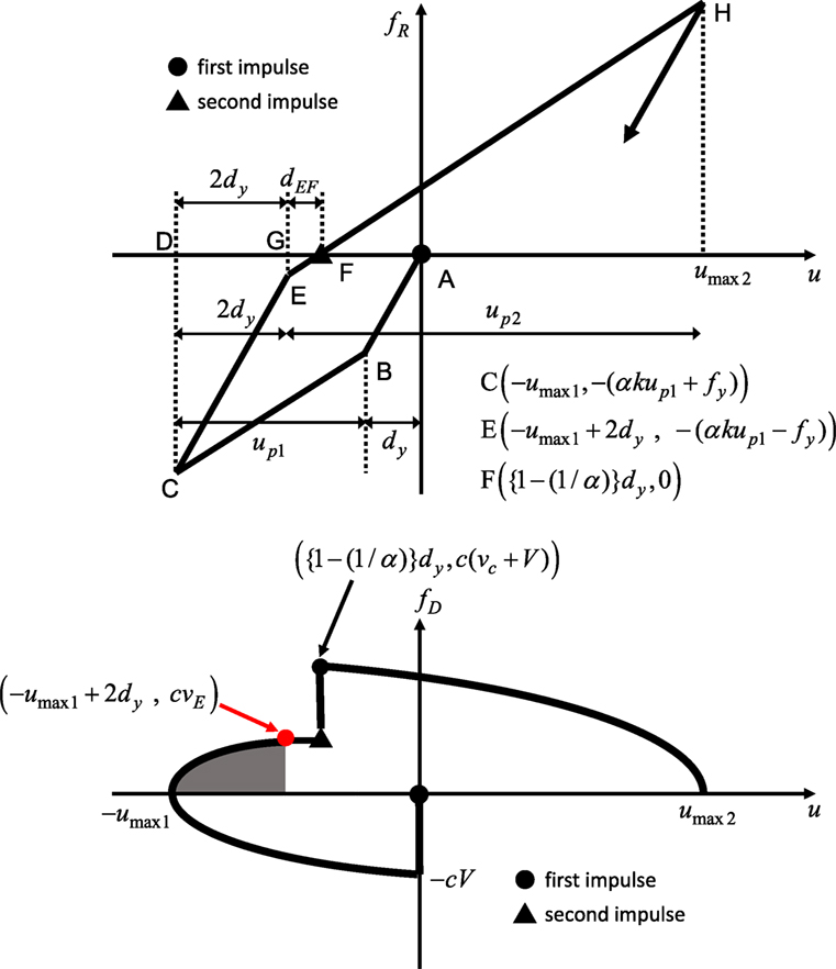
Figure 7. Evaluation of maximum elastic–plastic deformation under critical double impulse based on energy balance and quadratic function approximation of damping force–deformation relation for CASE 3-2 [(V/V_y)_{CASE 3} ≤ V/V_y].

The velocity v_E at point E in Figure 7 is derived by using the quadratic function approximation of the damping force–deformation relation. Point E is the point of the re-yielding initiation. The damping force–deformation relation between the point of the maximum deformation (point C) and the point of the re-yielding initiation (point E) can be approximated by a quadratic function which has the vertex (u, f_D) = (−u_max1, 0) and passes through the point (u, f_D) = (−u_max1 + 2d_y, cv_E). f_D can then be obtained as follows:

$f_D=c{v}_E\sqrt{\left(u+u_{\text{max}1}\right)/\left(2d_y\right)}.$ (28)

The work done by the damping force can be obtained by integrating Eq. 28 from u = − u_max1 to u = − u_max1 + 2d_y,

${\int }_{-u_{\text{max}1}}^{-u_{\text{max}1}+2d_y}{f}_D\mathit{du}=\left(2/3\right)c{v}_E\left(2d_y\right)=\left(4/3\right)c{v}_E{d}_y.$ (29)

The energy balance law between point C and E can be expressed as follows by using Eq. 29,

$\left(\text{area of CDGE}\right)=0.5m{v_E}^2+\left(4/3\right)c{v}_E{d}_y.$ (30)

The expression of (area of CDGE) in Eq. 30 indicates the area of the trapezoid CDGE in Figure 7. From Eq. 30, v_E can be obtained as

$v_E=V_y\left[-\left(8h/3\right)+\sqrt{\left(64h^2/9\right)+\mathrm{4\alpha }\left(u_{p1}/d_y\right)}\right].$ (31)

The velocity v_c at the zero-restoring-force timing after the first impulse (point F) is derived by solving the equation of motion in the reloading process. The equation of motion (free vibration) in the reloading process can be expressed as follows:

$\mathit{mü}+c\dot{u}+\mathrm{\alpha }\mathit{ku}+\left(1-\mathrm{\alpha }\right)k{d}_y=0.$ (32)

From Eq. 32, the deformation and velocity in the reloading process can be derived as follows by using the initial condition at point E where t = 0 is set at point E:

$u={\mathrm{e}}^{-h_2{\mathrm{\omega }}_{2}t}\sqrt{A^2+B^2}\text{sin}\left({\mathrm{\omega }}_2^{\prime }t-\mathrm{\theta }\right)+\left\{1-\left(1/\mathrm{\alpha }\right)\right\}{d}_y,$ (33)

$\dot{u}={\mathrm{\omega }}_2{\mathrm{e}}^{-h_2{\mathrm{\omega }}_{2}t}\sqrt{A^2+B^2}\text{cos}\left\{{\mathrm{\omega }}_2^{\prime }t-\mathrm{\theta }+\text{arctan}\left(h_2/\sqrt{1-{h_2}^2}\right)\right\},$ (34)

where

$A=\left(v_E-h_2{\mathrm{\omega }}_2{d}_{\mathit{EF}}\right)/{\mathrm{\omega }}_2^{\prime },$ (35)

$B=-d_{\mathit{EF}}=-\left[u_{\text{max}1}-\left\{1+\left(1/\mathrm{\alpha }\right)\right\}{d}_y\right],$ (36)

${\mathrm{\omega }}_2=\sqrt{\mathrm{\alpha }}{\mathrm{\omega }}_1,$ (37)

$h_2=\left(1/\sqrt{\mathrm{\alpha }}\right)h,$ (38)

${\mathrm{\omega }}_2^{\prime }=\sqrt{1-{h_2}^2}{\mathrm{\omega }}_2,$ (39)

$d_{\mathit{EF}}=u_{\text{max}1}-\left\{1+\left(1/\mathrm{\alpha }\right)\right\}{d}_y,$ (40)

$\mathrm{\theta }=\text{arccos}\left(A/\sqrt{A^2+B^2}\right).$ (41)

Since v_c is the velocity at the zero-restoring-force point (point F), where u = {1 − (1/α)}d_y, the time interval t_EF between the point E and F can be derived as follows from Eq. 33 and the condition u(t = t_EF) = {1 − (1/α)}d_y:

$t_{\mathit{EF}}=\mathrm{\theta }/{\mathrm{\omega }}_2^{\prime },$ (42)

v_c can be obtained by substituting Eq. 42 into t in Eq. 34,

$v_c={\mathrm{\omega }}_2^{\prime }{\mathrm{e}}^{-\left(h_2/\sqrt{1-{h_2}^2}\right)\mathrm{\theta }}\sqrt{A^2+B^2}.$ (43)

The maximum deformation u_max2 is derived next. t = 0 is set at point F and the displacement and velocity responses between point F and H can be obtained as follows by solving the equation of motion (Eq. 32) and substituting the initial condition at point F (after the second impulse),

$u=\left\{\left(v_c+V\right)/{\mathrm{\omega }}_2^{\prime }\right\}{\mathrm{e}}^{-h_2{\mathrm{\omega }}_{2}t}\text{sin}\left({\mathrm{\omega }}_2^{\prime }t\right)+\left\{1-\left(1/\mathrm{\alpha }\right)\right\}{d}_y,$ (44)

$\dot{u}=\left\{\left(v_c+V\right)/\sqrt{1-{h_2}^2}\right\}{\mathrm{e}}^{-h_2{\mathrm{\omega }}_{2}t}\text{cos}\left\{{\mathrm{\omega }}_2^{\prime }t+\text{arctan}\left(h_2/\sqrt{1-h^2}\right)\right\}.$ (45)

The deformation response after the second impulse is maximized at the time at which $\dot{u}=0$. From Eq. 45 and $\dot{u}=0$, the time interval t_max2 between point F and H can be obtained as follows:

$t_{\text{max}2}=\left\{0.\mathrm{5\pi }-\text{arctan}\left(h_2/\sqrt{1-{h_2}^2}\right)\right\}/{\mathrm{\omega }}_2^{\prime }.$ (46)

Therefore, u_max2 can be obtained as follows by substituting Eq. 46 into t in Eq. 44,

$u_{\text{max}2}/d_y=1-\left(1/\mathrm{\alpha }\right)+\left(1/\sqrt{\mathrm{\alpha }}\right)\left\{\left(v_c+V\right)/V_y\right\}\text{exp}\left[-\left(h_2/\sqrt{1-{h_2}^2}\right)\left\{0.\mathrm{5\pi }-\text{arctan}\left(h_2/\sqrt{1-{h_2}^2}\right)\right\}\right].$ (47)

Critical Impulse Timing

The critical time intervals $t_0^c$ between two impulses are derived in this section. In contrast to the previous papers dealing with the model without viscous damping, it is difficult to derive an analytical expression on the critical time interval between two impulses in CASE 3-1 and CASE 3-2. For this reason, the time-history response analysis is used under the first impulse and the time interval is computed as the time up to the zero-restoring-force timing. It is necessary to use different expressions in the previous sections on the maximum deformation depending on the input velocity level.

Figure 8 illustrates the normalized time interval $t_0^c$ for T₁ with respect to the input velocity level of the double impulse for various post-yield stiffness ratios α = 0.1, 0.3, 0.5 and various damping ratios h = 0.05, 0.1, 0.2. In CASE 1 and CASE 2, the critical time interval is obtained by $t_0^c=T_1^{\prime }/2$. Therefore, as the damping ratio becomes larger, the critical time interval becomes longer. In CASE 3, as the damping ratio becomes larger, the plastic deformation u_p1 after the first impulse becomes smaller and the critical time interval $t_0^c$ becomes shorter. It can be observed that, as the post-yield stiffness ratio becomes larger, CASE 3-2 appears in the smaller level of the input velocity of the double impulse. The sudden change of slope indicates the transition of CASE 2, CASE 3-1, and CASE 3-2.

FIGURE 8

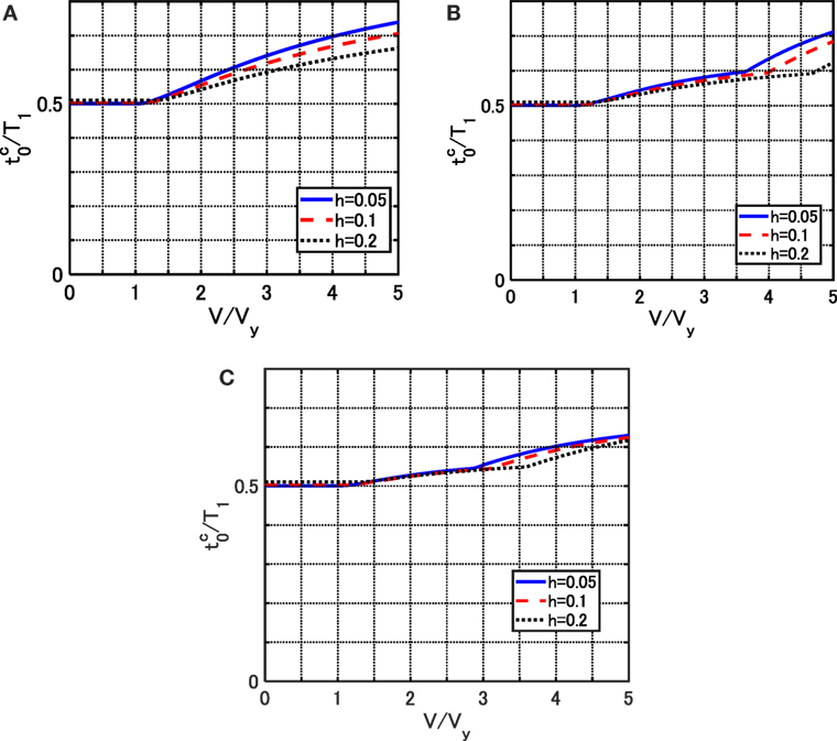
Figure 8. Normalized critical impulse timing $t_{\text{0}}^c/T_{\text{1}}$ with respect to input level V/V_y for various post-yield stiffness ratios α, (A) α = 0.1, (B) α = 0.3, and (C) α = 0.5.

Accuracy Check of the Proposed Expression Under the Double Impulse through the Comparison with the Time-History Response Analysis Under the Double Impulse and the Corresponding One-Cycle Sinusoidal Wave

To check the accuracy of the proposed expression under the double impulse, the time-history response analyses of the SDOF damped bilinear hysteresis system under the double impulse and the corresponding one-cycle sinusoidal wave have been conducted. In the time-history response analysis under the critical double impulse, the second impulse acts at the timing of zero-restoring-force. The validity of this assumption on the critical timing of the second impulse will be investigated in Section “Proof of Critical Timing.”

In this evaluation, it is important to adjust the input levels between the double impulse and the corresponding one-cycle sinusoidal wave based on the equivalence of the maximum Fourier amplitude. The adjustment procedure is explained in Appendix 1. The one-cycle sine wave that corresponds to the critical double impulse can be represented as follows:

${ü}_g^{\text{SW}}\left(t\right)=0.5{\mathrm{\omega }}_p{V}_p\text{sin}\left({\mathrm{\omega }}_{p}t\right)\left(0\le t\le T_p=2t_0^c\right),$ (48)

where V_p/V = 1.2222 (Kojima and Takewaki, 2016, Kojima et al., 2017). In addition, $T_p=2t_0^c$ and ω_p = 2π/$T_p$ denote the period and the circular frequency, respectively, of the sine wave. The critical time interval obtained in Section “Critical Impulse Timing” is used for $t_0^c$ in Eq. 48.

Figures 9–11 present the comparison of the maximum deformations of the models for α = 0.1, 0.3, 0.5 and h = 0.05, 0.1, 0.2. It can be observed from the comparison with the time-history response analysis under the critical double impulse that the closed-form solution of u_max2 based on the quadratic function approximation of the damping force–deformation relation of the dashpot is accurate enough. Furthermore, from the comparison with the time-history response analysis under the corresponding one-cycle sine wave, the approximate closed-form solution of u_max2 is in good agreement with the time-history response analysis under the corresponding one-cycle sine wave and the closed-form solution of u_max1 based on the quadratic function approximation of the damping force–deformation relation of the dashpot provides a narrow upper bound for the result by the time-history response analysis under the corresponding one-cycle sine wave.

FIGURE 9

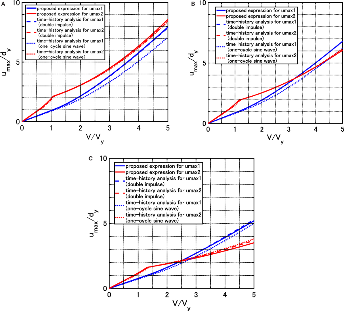
Figure 9. Comparison of maximum deformations for model of α = 0.1 among proposed method, time-history response analysis under double impulse and time-history response analysis under corresponding one-cycle sine wave, (A) h = 0.05, (B) h = 0.1, and (C) h = 0.2.

FIGURE 10

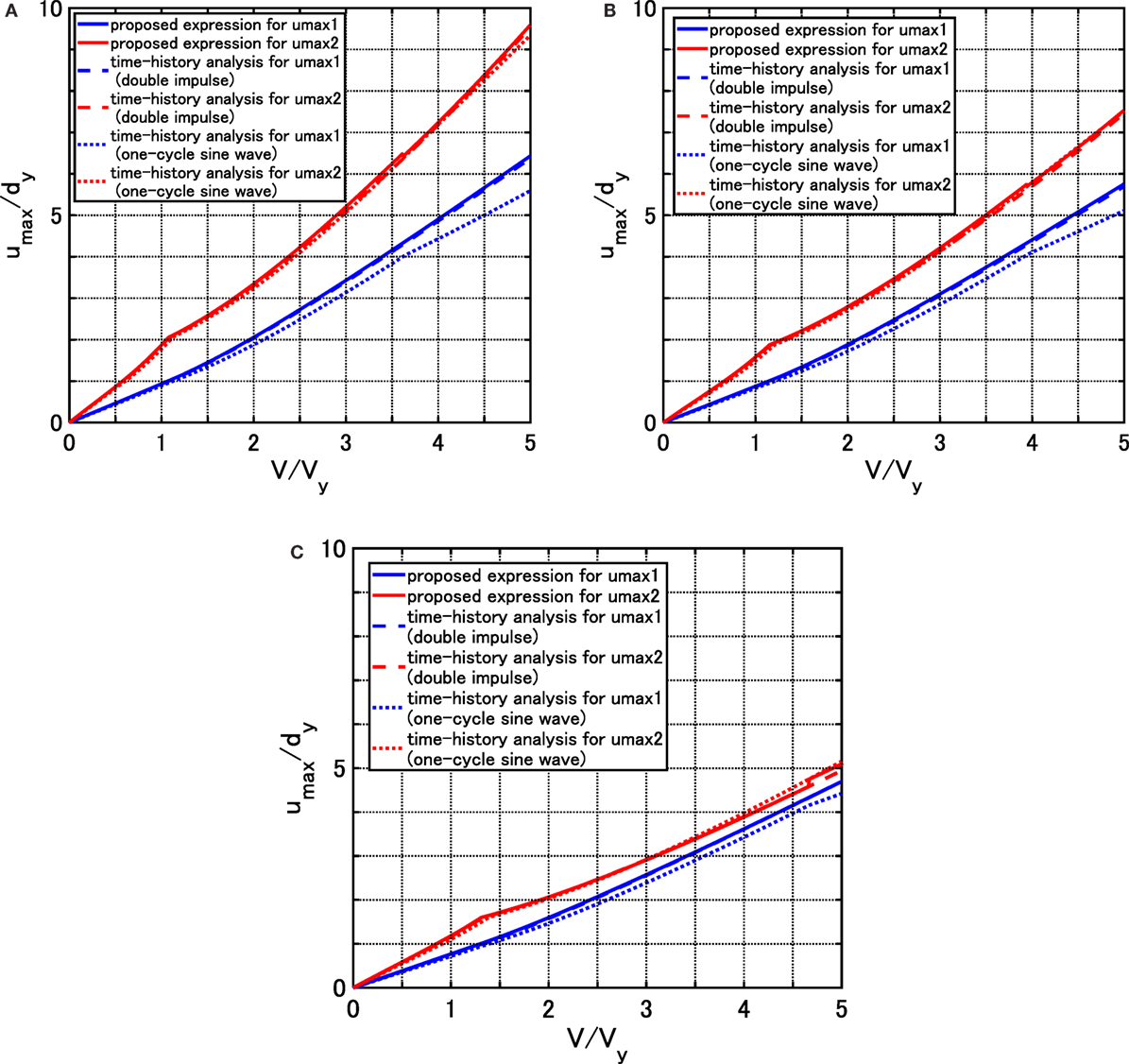
Figure 10. Comparison of maximum deformations for model of α = 0.3 among proposed method, time-history response analysis under double impulse and time-history response analysis under corresponding one-cycle sine wave, (A) h = 0.05, (B) h = 0.1, and (C) h = 0.2.

FIGURE 11

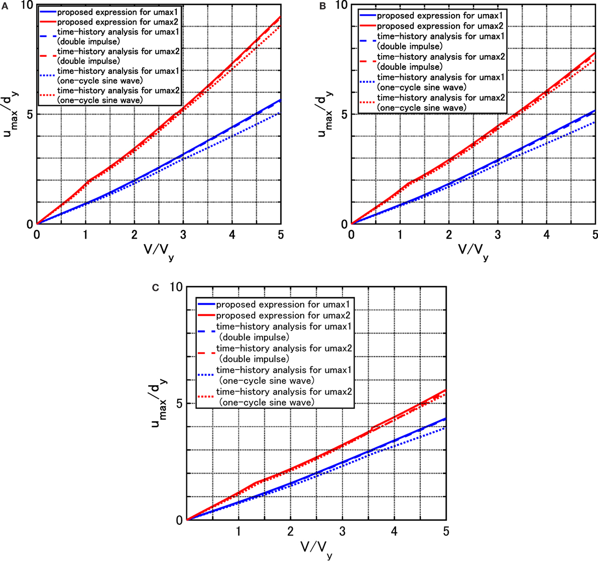
Figure 11. Comparison of maximum deformations for model of α = 0.5 among proposed method, time-history response analysis under double impulse and time-history response analysis under corresponding one-cycle sine wave, (A) h = 0.05, (B) h = 0.1, and (C) h = 0.2.

Proof of Critical Timing

The validity of the assumption that the critical timing of the second impulse is the zero-restoring-force timing is investigated in this section. Figure 12 shows the normalized maximum deformation $u_{\text{max}2}/u_{\text{max}2}^c$ with respect to the normalized timing $t_0/t_0^c$ of the second impulse under constant input velocity and the time history of restoring force under a single impulse, i.e., the first impulse, for two cases, CASE 3-1 (α = 0.5, h = 0.05, V/V_y = 2.0) and CASE 3-2 (α = 0.5, h = 0.05, V/V_y = 4.0). u_max2 in Figure 12 denotes the maximum deformation after the second impulse under the double impulse with an arbitrary time interval t₀. In Figure 12, $t_0^c$ was obtained following the procedure explained in Section “Critical Impulse Timing” and $u_{\text{max}2}^c$ denotes the maximum deformation after the second impulse under the critical double impulse (the maximum value of u_max2) calculated by the time-history response analysis. It can be seen that the zero-restoring-force timing after the first impulse just corresponds to the critical timing providing the maximum deformation $u_{\text{max}2}=u_{\text{max}2}^c$.

FIGURE 12

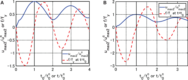
Figure 12. Maximum deformation with respect to timing of second impulse under constant input velocity and time history of restoring force under first single impulse, (A) CASE 3-1 (α = 0.5, h = 0.05, V/V_y = 2.0) and (B) CASE 3-2 (α = 0.5, h = 0.05, V/V_y = 4.0).

Accuracy Check of the Response Under the Critical Double Impulse through the Comparison with the Time-History Response Under the Corresponding One-Cycle Sinusoidal Wave

To demonstrate the validity of using the double impulse as a substitute for one-cycle sine wave which represents a main part of the near-fault ground motion, the comparison between the responses under the critical double impulse and the corresponding one-cycle sine wave is conducted in this section. Figures 13A–C show the comparison of the deformation time history, the restoring force time history and the force–deformation relation under the critical double impulse and the corresponding one-cycle sine wave for the model of α = 0.3, h = 0.1 and the input level of V/V_y = 3.0. It should be noted that the phase lag was adjusted to compare appropriately the time-history responses under the critical double impulse and the corresponding one-cycle sine wave. It can be observed that the response under the critical double impulse is a good approximation of the response under the corresponding one-cycle sine wave. This supports the validity of the proposed expression under the critical double impulse.

FIGURE 13

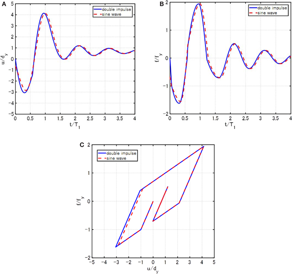
Figure 13. Comparison of the responses under the critical double impulse and the equivalent one-cycle sine wave for the model of α = 0.3, h = 0.1 and the input level of V/V_y = 3.0, (A) deformation time history, (B) restoring-force time history, and (C) force–deformation relation.

Application of Proposed Expression on Critical Response to Recorded Near-Fault Ground Motion

To investigate the applicability of the proposed theory to actual recorded ground motions, the comparison of the critical elastic–plastic response has been conducted under a near-fault ground motion and under the critical double impulse. The Rinaldi station fault-normal component during the Northridge earthquake in 1994 shown in Figure 1A is used as the near-fault ground motion.

It should be noted that the critical double impulse was determined for given structural parameters represented by V_y in Section “Closed-Form Expression of Maximum Elastic–Plastic Response under Critical Double Impulse.” On the contrary, in this section, the structural parameters are chosen so as to maximize the response for a fixed input velocity V of the real recorded ground motion. This treatment is somewhat similar to the well-known elastic–plastic response spectrum which was proposed in 1960s and was conducted by changing the strength parameter of an elastic–plastic structure. The input velocity level of the double impulse corresponding to the Rinaldi station fault-normal component is V = 1.64 m/s.

The procedure of evaluating the critical response under the recorded ground motion is explained here. The main part of the recorded ground motion is approximated by a one-cycle sinusoidal wave as shown in Figure 1A. The acceleration amplitude, the maximum velocity and the period of the approximated one-cycle sinusoidal wave for the Rinaldi station fault-normal component are A_p = 7.85 m/s², V_p = 2.0 m/s, T_p = 0.8 s, respectively. From V_p = 2.0 m/s and V_p/V = 1.2222, the input velocity level of the double impulse corresponding to the Rinaldi station fault-normal component is V = 1.64 m/s. From the period $T_p=2t_0^c$ of the one-cycle sinusoidal wave and the specified value of V/V_y, the natural period of the SDOF system can be obtained. The relation between V/V_y and $t_0^c/T_1$ can be obtained by the procedure explained in Section “Critical Impulse Timing.” V_y can be obtained from the specified value of V/V_y and the input velocity level V of the double impulse corresponding to the recorded ground motion, and the yield deformation d_y can be obtained from V_y and ω₁ = 2π/T₁. These values of T₁, ω₁, and d_y are the parameters of the approximate critical SDOF system under the recorded ground motion for the specified value of V/V_y. The response of this critical system (the system exhibiting the maximum response) under the recorded ground motion is calculated by using the time-history response analysis.

Figures 14A–D show the comparison of the amplitude of critical elastic–plastic response under the Rinaldi station fault-normal component by time-history response analysis with the proposed explicit expression of the amplitude of elastic–plastic response under the critical double impulse. The vertical axis indicates the maximum amplitude of elastic–plastic deformation (the sum of u_max1 and u_max2), and the horizontal axis presents the input velocity level expressed by V/V_y. It can be observed that the amplitude of elastic–plastic response of a damped bilinear hysteretic structure under the critical double impulse coincides fairly well with the amplitude of elastic–plastic response under the actual recorded ground motion in a broad range of the input level.

FIGURE 14

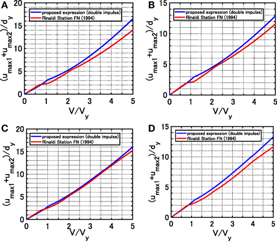
Figure 14. Comparison of maximum amplitude of deformation of models with α = 0.1, 0.3, h = 0.05, 0.1 under critical double impulse (using quadratic function approximation) and recorded ground motion (Rinaldi Sta. FN comp.), (A) α = 0.1, h = 0.05, (B) α = 0.1, h = 0.1, (C) α = 0.3, h = 0.05, and (D) α = 0.3, h = 0.1.

Conclusion

The double impulse has been used as a good substitute for a one-cycle sine wave which represents a main part of the near-fault ground motion and the explicit expression on the maximum elastic–plastic response has been derived for the SDOF damped bilinear hysteretic system subjected to the critical double impulse. In the past conventional approach using the sinusoidal wave (Iwan, 1961), the equivalent frequency resonant to the elastic–plastic system for a specified input level must be computed iteratively by varying the input frequency parametrically. Compared with this approach, the maximum elastic–plastic response under the critical double impulse, which causes the maximum response for variable time interval of impulses, can be derived explicitly without repetitive procedure in the proposed method. Furthermore the critical time interval of two impulses in the double impulse (the resonant frequency) can also be determined systematically depending on the input level. The conclusions may be summarized as follows:

(1) The energy balance approach and the quadratic function approximation of the damping force–deformation relation of the dashpot enabled the explicit expressions on the maximum elastic–plastic response under the critical double impulse. The maximum response under the critical double impulse can be classified into four cases depending on the input level. CASE 1 is the case where the model remains elastic even after the second impulse and CASE 2 is the case where the model goes into the plastic range only after the second impulse. Furthermore CASE 3 is the case where the model goes into the plastic range even after the first impulse. In CASE 3, there are two more cases, i.e., CASE 3-1 where the zero-restoring-force timing after the first impulse exists in the unloading stage and CASE 3-2 where the zero-restoring-force timing after the first impulse exists in the reloading stage after the unloading stage.

(2) The accuracy of the derived expressions has been discussed through the comparison with the maximum response under the critical double impulse and the equivalent one-cycle sine wave as a good representative for the near-fault ground motion. The time-history response analysis has been used for reliable comparison. It has been demonstrated that the double impulse can be a good substitute for the one-cycle sine wave after appropriate adjustment of the maximum Fourier amplitude and the maximum deformation under a near-fault ground motion can be obtained by using the double impulse.

(3) The validity of the critical time interval of two impulses derived in Section “Critical Impulse Timing” has been investigated by conducting the time-history response analysis of the SDOF damped bilinear hysteresis system under the double impulse. The impulse timing has been varied continuously. It was made clear that the critical timing of the second impulse is the timing with zero restoring force after the first impulse (unloading process or reloading process).

The proposed method can be extended to the problem of critical excitation for a base-isolated building structure on ground under a near-fault ground motion by reducing this system into an SDOF system. When the base-isolation story possesses a bilinear hysteretic restoring-force characteristic and the super-structure and ground can be modeled using elastic elements, the total system can be simplified into an SDOF system with a bilinear hysteretic restoring-force characteristic. After the total response of this SDOF system is evaluated by using the present method, the maximum deformation of the base-isolation story and other response can be evaluated by using the relation between the total response and each substructure.

In addition, the proposed method can be extended to the problem of rocking of flexible structures (Vassiliou et al., 2016). As for the problem of rocking of rigid blocks, some important achievements have been made (Casapulla, 2015; Nabeshima et al., 2016; Casapulla and Maione, 2017; Taniguchi et al., 2017). The combination of these achievements with the present formulation may lead to the formulation for the problem of rocking of flexible inelastic structures.

Author Contributions

HA formulated the problem, conducted the computation, and wrote the paper. KK formulated the problem and wrote the paper. IT supervised the research and wrote the paper.

Conflict of Interest Statement

The authors declare that the research was conducted in the absence of any commercial or financial relationships that could be construed as a potential conflict of interest.

Funding

Part of the present work is supported by KAKENHI of Japan Society for the Promotion of Science (No. 15H04079, 15J00960, 17J00407) and Sumitomo Rubber Industries, Co. This support is greatly appreciated.

References

Abrahamson, N., Ashford, S., Elgamal, A., Kramer, S., Seible, F., and Somerville, P. (1998). Proc. of the 1st PEER Workshop on Characterization of Special Source Effects. San Diego: Pacific Earthquake Engineering Research Center, University of California, 1998.

Google Scholar

Alavi, B., and Krawinkler, H. (2004). Behaviour of moment resisting frame structures subjected to near-fault ground motions. Earthquake Eng. Struct. Dyn. 33, 687–706. doi:10.1002/eqe.370

CrossRef Full Text | Google Scholar

Bertero, V. V., Mahin, S. A., and Herrera, R. A. (1978). Aseismic design implications of near-fault San Fernando earthquake records. Earthquake Eng. Struct. Dyn. 6, 31–42. doi:10.1002/eqe.4290060105

CrossRef Full Text | Google Scholar

Casapulla, C. (2015). On the resonance conditions of rigid rocking blocks. Int. J. Eng. Technol. 7, 760–771.

Google Scholar

Casapulla, C., and Maione, A. (2017). Critical response of free-standing rocking blocks to the intense phase of an earthquake. Int. Rev. Civil Eng. 8, 1–10. doi:10.15866/irece.v8i1.11024

CrossRef Full Text | Google Scholar

Caughey, T. K. (1960a). Sinusoidal excitation of a system with bilinear hysteresis. J. Appl. Mech. 27, 640–643. doi:10.1115/1.3644075

CrossRef Full Text | Google Scholar

Caughey, T. K. (1960b). Random excitation of a system with bilinear hysteresis. J. Appl. Mech. 27, 649–652. doi:10.1115/1.3644077

CrossRef Full Text | Google Scholar

Drenick, R. F. (1970). Model-free design of aseismic structures. J. Eng. Mech. Div. 96, 483–493.

Google Scholar

Hall, J. F., Heaton, T. H., Halling, M. W., and Wald, D. J. (1995). Near-source ground motion and its effects on flexible buildings. Earthuake Spectra 11, 569–605. doi:10.1193/1.1585828

CrossRef Full Text | Google Scholar

Iwan, W. D. (1961). The Dynamic Response of Bilinear Hysteretic Systems. Ph.D. thesis, California Institute of Technology, Pasadena.

Google Scholar

Iwan, W. D. (1965a). “The dynamic response of the one-degree-of-freedom bilinear hysteretic system,” in Proc. of the Third World Conf. on Earthquake Eng (New Zealand).

Google Scholar

Iwan, W. D. (1965b). The steady-state response of a two-degree-of-freedom bilinear hysteretic system. J. Appl. Mech. 32, 151–156. doi:10.1115/1.3625711

CrossRef Full Text | Google Scholar

Kalkan, E., and Kunnath, S. K. (2006). Effects of fling step and forward directivity on seismic response of buildings. Earthquake Spectra 22, 367–390. doi:10.1193/1.2192560

CrossRef Full Text | Google Scholar

Khaloo, A. R., Khosravi, H., and Hamidi Jamnani, H. (2015). Nonlinear interstory drift contours for idealized forward directivity pulses using “modified fish-bone” models. Adv. Struct. Eng. 18, 603–627. doi:10.1260/1369-4332.18.5.603

CrossRef Full Text | Google Scholar

Kojima, K., Saotome, Y., and Takewaki, I. (2017). Critical earthquake response of a SDOF elastic-perfectly plastic model with viscous damping under double impulse as a substitute of near-fault ground motion. J. Struct. Construct. Eng. 735, 643–652. doi:10.3130/aijs.82.643

CrossRef Full Text | Google Scholar

Kojima, K., and Takewaki, I. (2015a). Critical earthquake response of elastic-plastic structures under near-fault ground motions (part 1: fling-step input). Front. Built Environ. 1:12. doi:10.3389/fbuil.2015.00012

CrossRef Full Text | Google Scholar

Kojima, K., and Takewaki, I. (2015b). Critical earthquake response of elastic-plastic structures under near-fault ground motions (part 2: forward-directivity input). Front. Built Environ. 1:13. doi:10.3389/fbuil.2015.00013

CrossRef Full Text | Google Scholar

Kojima, K., and Takewaki, I. (2015c). Critical input and response of elastic-plastic structures under long-duration earthquake ground motions. Front. Built Environ. 1:15. doi:10.3389/fbuil.2015.00015

CrossRef Full Text | Google Scholar

Kojima, K., and Takewaki, I. (2016). Closed-form critical earthquake response of elastic-plastic structures with bilinear hysteresis under near-fault ground motions. J. Struct. Construct. Eng. 726, 1209–1219. doi:10.3130/aijs.81.1209

CrossRef Full Text | Google Scholar

Liu, C.-S. (2000). The steady loops of SDOF perfectly elastoplastic structures under sinusoidal loadings. J. Mar. Sci. Technol. 8, 50–60.

Google Scholar

Makris, N., and Black, C. J. (2004). Dimensional analysis of rigid-plastic and elastoplastic structures under pulse-type excitations. J. Eng. Mech. 130, 1006–1018. doi:10.1061/(ASCE)0733-9399(2004)130:9(1019)

CrossRef Full Text | Google Scholar

Mavroeidis, G. P., Dong, G., and Papageorgiou, A. S. (2004). Near-fault ground motions, and the response of elastic and inelastic single-degree-freedom (SDOF) systems. Earthquake Eng. Struct. Dyn. 33, 1023–1049. doi:10.1002/eqe.391

CrossRef Full Text | Google Scholar

Mavroeidis, G. P., and Papageorgiou, A. S. (2003). A mathematical representation of near-fault ground motions. Bull. Seism. Soc. Am. 93, 1099–1131. doi:10.1785/0120020100

CrossRef Full Text | Google Scholar

Nabeshima, K., Taniguchi, R., Kojima, K., and Takewaki, I. (2016). Closed-form overturning limit of rigid block under critical near-fault ground motions. Front. Built Environ. 2:9. doi:10.3389/fbuil.2016.00009

CrossRef Full Text | Google Scholar

Roberts, J. B., and Spanos, P. D. (1990). Random Vibration and Statistical Linearization. New York, NY: Wiley.

Google Scholar

Sasani, M., and Bertero, V. V. (2000). “Importance of severe pulse-type ground motions in performance-based engineering: historical and critical review,” in Proc. of the Twelfth World Conference on Earthquake Engineering (Auckland, New Zealand).

Google Scholar

Takewaki, I. (2007). Critical Excitation Methods in Earthquake Engineering, 2nd ed. London: Elsevier, 2013.

Google Scholar

Takewaki, I., Murakami, S., Fujita, K., Yoshitomi, S., and Tsuji, M. (2011). The 2011 off the Pacific coast of Tohoku earthquake and response of high-rise buildings under long-period ground motions. Soil Dyn. Earthquake Eng. 31, 1511–1528. doi:10.1016/j.soildyn.2011.06.001

CrossRef Full Text | Google Scholar

Taniguchi, R., Nabeshima, K., Kojima, K., and Takewaki, I. (2017). Closed-form rocking vibration of rigid block under critical and non-critical double impulse. Int. J. Earthquake Impact Eng. 2, 32–45. doi:10.1504/IJEIE.2017.083708

CrossRef Full Text | Google Scholar

Vassiliou, M. F., Mackie, K. R., and Stojadinović, B. (2016). A finite element model for seismic response analysis of deformable rocking frames. Earthquake Eng. Struct. Dyn. 46, 447–466. doi:10.1002/eqe.2799

CrossRef Full Text | Google Scholar

Appendix 1

Double Impulse and Corresponding One-Cycle Sine Wave with the Same Frequency and the Same Maximum Fourier Amplitude

The velocity amplitude V of the double impulse is related to the maximum velocity of the corresponding one-cycle sine wave with the same frequency (the period is twice the interval of the double impulse) so that the maximum Fourier amplitudes of both inputs coincide.

The double impulse is expressed by

${ü}_g\left(t\right)=V\mathrm{\delta }\left(t\right)-V\mathrm{\delta }\left(t-t_0\right).$ (A1)

The Fourier transform of Eq. A1 can be obtained as

${Ü}_g\left(\mathrm{\omega }\right)=V\left(1-e^{-i\mathrm{\omega }{t}_0}\right).$ (A2)

Let A_p, T_p, and ω_p = 2π/T_p denote the acceleration amplitude, the period and the circular frequency of the corresponding one-cycle sine wave, respectively. The acceleration wave ${ü}_g^{\text{SW}}$ of the corresponding one-cycle sine wave is expressed by

${ü}_g^{\text{SW}}=A_p\text{sin}\left({\mathrm{\omega }}_{p}t\right)\left(0\le t\le T_p=2t_0\right).$ (A3)

The time interval t₀ of two impulses in the double impulse is related to the period T_p of the corresponding one-cycle sine wave by T_p = 2t₀. Although the starting points of both inputs differ by t₀/2, the starting time of one-cycle sine wave does not affect the Fourier amplitude. For this reason, the starting time of one-cycle sine wave will be adjusted so that the responses of both inputs correspond well. In this appendix, the relation of the velocity amplitude V of the double impulse with the acceleration amplitude A_p of the corresponding one-cycle sine wave is derived. The ratio a of A_p to V is introduced by

$A_p=\mathit{aV}.$ (A4)

The Fourier transform of ${ü}_g^{\text{SW}}$ in Eq. A3 is computed by

${Ü}_g^{\text{SW}}\left(\mathrm{\omega }\right)={\int }_0^{2t_0}\left\{A_p\text{sin}\left({\mathrm{\omega }}_{p}t\right)\right\}{\mathrm{e}}^{-i\mathrm{\omega }t}\mathit{dt}=\frac{\mathrm{\pi }{t}_0{A}_p}{{\mathrm{\pi }}^2-{\left(\mathrm{\omega }{t}_0\right)}^2}\left(1-{\mathrm{e}}^{-2t_0\mathrm{\omega }i}\right).$ (A5)

From Eqs A2 and A5, the Fourier amplitudes of both inputs are expressed by

$\left|{Ü}_g\left(\mathrm{\omega }\right)\right|=V\sqrt{2-2\text{cos}\left(\mathrm{\omega }{t}_0\right)},$ (A6)

$\left|{Ü}_g^{\text{SW}}\left(\mathrm{\omega }\right)\right|=A_p\left|\frac{\mathrm{2\pi }{t}_0}{{\mathrm{\pi }}^2-{\left(\mathrm{\omega }{t}_0\right)}^2}\text{sin}\left(\mathrm{\omega }{t}_0\right)\right|.$ (A7)

The coefficient a can be derived from Eqs A4, A6, and A7 and the equivalence of the maximum Fourier amplitude ${\left|{Ü}_g\left(\mathrm{\omega }\right)\right|}_{\text{max}}={\left|{Ü}_g^{\text{SW}}\left(\mathrm{\omega }\right)\right|}_{\text{max}}$,

$a\left(t_0\right)=\frac{A_p}{V}=\frac{\text{max}\left|\sqrt{2-2\text{cos}\left(\mathrm{\omega }{t}_0\right)}\right|}{\text{max}\left|\frac{\mathrm{2\pi }{t}_0}{{\mathrm{\pi }}^2-{\left(\mathrm{\omega }{t}_0\right)}^2}\text{sin}\left(\mathrm{\omega }{t}_0\right)\right|}.$ (A8)

In Eq. A8, $\text{max}\left|\sqrt{2-2\text{cos}\left(\mathrm{\omega }{t}_0\right)}\right|=2$ holds. The denominator $\text{max}\left|\mathrm{2\pi }{t}_0\text{sin}\left(\mathrm{\omega }{t}_0\right)/\left\{{\mathrm{\pi }}^2-{\left(\mathrm{\omega }{t}_0\right)}^2\right\}\right|$ in Eq. A8 will be evaluated next.

Let us define the function f (x) given by

$f\left(x\right)=\frac{1}{{\mathrm{\pi }}^2-x^2}\text{sin}x.$ (A9)

The maximum value f_max of f (x) and the corresponding argument x = x₀ can be obtained as follows:

$x_0=2.63099585\dots ,$ (A10)

$f_{\text{max}}=f\left(x=x_0\right)=0.165802809\dots .$ (A11)

The values in Eqs A10 and A11 were obtained numerically. From Eqs A8 and A11, the coefficient a is expressed as a function of the time interval t₀ of two impulses,

$a\left(t_0\right)=1/\left(\mathrm{\pi }{t}_0{f}_{\text{max}}\right).$ (A12)

Figure A1A shows the relation between t₀ and a. Furthermore Figure A1B presents examples of the Fourier amplitudes of both inputs with the same maximum Fourier amplitude. Since the Fourier amplitudes of both inputs differ greatly in larger frequencies, further investigation will be necessary in dealing with multi-degree-of-freedom models in the future.

FIGURE A1

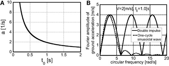
Figure A1. Relation of amplitudes between double impulse and one-cycle sine wave, (A) coefficient a, (B) Fourier amplitude of double impulse and one-cycle sine wave.

Consider next the ratio of the maximum velocity V_p of one-cycle sine wave to the velocity amplitude V of the double impulse. The velocity function ${\dot{u}}_g^{\text{SW}}$ of one-cycle acceleration sine wave is expressed by

${\dot{u}}_g^{\text{SW}}={\int }_0^t{ü}_g^{\text{SW}}\mathit{dt}={\int }_0^t{A}_p\text{sin}\left({\mathrm{\omega }}_{p}t\right)\mathit{dt}=\frac{A_p}{{\mathrm{\omega }}_p}\left\{1-\text{cos}\left({\mathrm{\omega }}_{p}t\right)\right\}.$ (A13)

From Eq. A13, the maximum velocity V_p of one-cycle sine wave can be expressed by

$V_p=2A_p/{\mathrm{\omega }}_p.$ (A14)

Equations A12 and A14 lead to the relation between V_p and V,

$V_p=\left\{2/\left({\mathrm{\pi }}^2{f}_{\text{max}}\right)\right\}V.$ (A15)

From Eqs A11 and A15, V_p/V can be obtained as

$V_p/V=2/\left({\mathrm{\pi }}^2{f}_{\text{max}}\right)=1.22218898\dots .$ (A16)

It can be found from Eq. A16 that, if the maximum Fourier amplitudes of both inputs are the same, the ratio of V_p to V becomes constant. The modulated one-cycle sine wave will be called “the corresponding one-cycle sine wave.”