A Meshless Solution to the Vibration Problem of Cylindrical Shell Panels

Introduction

Thin shell structures have an outstanding efficiency in fully utilizing the structural material and have been extensively used in many engineering applications including aircraft structures, pressure vessels, and others. Static and dynamic analysis is essential for the analysis and design of shell structures. Various numerical methods, such as the Finite Difference Method (FDM) and especially the Finite Element Method (FEM) have been used (Lee and Han, 2001) for the dynamic analysis of linear elastic thin shells characterized by complex geometry, loading and boundary conditions. Both methods have been employed successfully for the solution of a variety of static and dynamic shell problems. The Boundary Element Method (BEM) is an efficient alternative to the domain type methods, especially for thin elastic shallow shells (Beskos, 1991), or combined with the AEM for cylindrical shells (Yiotis and Katsikadelis, 2000).

Such methods require the generation of a mesh which can be an incredibly tedious and time-consuming process, while their convergence rate is of 2nd order (Cheng et al., 2003). On the other hand, Meshless Methods (MMs) present an attractive alternative to FEM or BEM, especially for shell structures that are complex regarding both the governing equations and the geometry representation. Comprehensive descriptions of different MMs are presented by Liu (2002); Liu and Gu (2005) and in a review paper by Nguyen et al. (2008).

There are several papers on dynamic analysis of shells using MM. Homogeneous shells are studied using various versions of MM in Liu et al. (2006), Ferreira et al. (2006b), and Dinis et al. (2011). Functionally graded (FG) cylindrical thin shells have also been treated by this method (Ferreira et al., 2006a; Zhao et al., 2009; Roque et al., 2010), as well as thick cylindrical shells (Pilafkan et al., 2013) have been analyzed by this method.

The mesh-free multiquadric radial basis functions (MQ-RBFs) method presented in Kansa (2005) has attracted the interest of researchers, due to its exponential convergence and its easiness of implementation. The significant drawbacks of the method are the ill-conditioning of the coefficient matrix and the inability to accurately approximate the derivatives of the sought solution which renders the method inappropriate for a strong formulation of the problem. These drawbacks of the standard MQ-RBF method, are overcome by a new RBF method presented recently by Katsikadelis (2006, 2008a,b, 2009) and Yiotis and Katsikadelis (2008, 2013, 2015a,b). Another critical issue is the implementation of multiple boundary conditions for equations of order higher than 2nd. In this investigation, the δ-technique is employed (Jang et al., 1989) for the 4th order equation. The problem of multiple boundary conditions is not present when the shell is modeled as a 3D body (Katsikadelis and Platanidi, 2007).

In this paper, the MAEM is extended to the dynamic problem of cylindrical shell panels as described by section MAEM Solution. A first approach to this problem was attempted in a previous work (Yiotis and Katsikadelis, 2015b), where some preliminary results only for the eigenfrequency analysis were presented. In section Problem Statement, the statement of the problem is presented, while several example problems are worked out in section Numerical Examples, which illustrate the applicability of the method and demonstrate its efficiency and section Conclusions contains certain conclusions drawn from this investigation.

Problem Statement

We consider a thin cylindrical shell with parametric lines x (s = const.) and s (x = const.) which are assumed to be lines of curvature, as well; x is measured along the x lines of the shell and s along the s lines, while z is measured along the normal to the middle surface of the shell, as shown in Figure 1. R is the radius of curvature and h is the thickness.

FIGURE 1

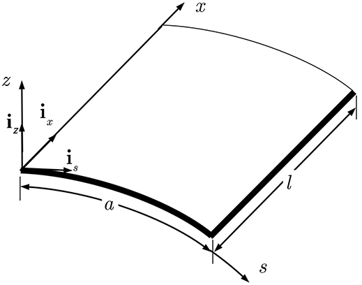
Figure 1. Cylindrical shell.

In this investigation we use the Flügge equations for the thin shell theory, based on the following assumptions (Love, 1944):

1. The thickness of the shell is small compared with (i) its other dimensions; (ii) the smallest radius of the shell curvature.

2. Strains and displacements are sufficiently small and as a result quantities of 2nd and higher order of magnitude in the strain-displacement relations can be neglected.

3. The normal transverse stress is relatively small, compared with the other normal stresses, and can be neglected.

4. Lines normal to the undeformed middle surface remain straight and normal to the deformed middle surface.

The first assumption defines the meaning of “thin shells,” whereas the second one implies that all calculations refer to the original undeformed configuration and subsequently leads to linear differential equations. Further, the assumption z/R < < 1 is adopted in deriving the stress resultants in integrating the stresses through the thickness of the shell. The 4th assumption is known as Kirchhoff's hypothesis yielding

$\begin{array}{rcll}{\gamma }_{xz}& =& 0,& (\mathrm{1a})\end{array}$

$\begin{array}{rcll}{\gamma }_{sz}& =& 0,& (\mathrm{1b})\end{array}$

$\begin{array}{rcll}{e}_z& =& 0,& (\mathrm{1c})\end{array}$

which implies σ_xz = σ_sz = 0 (Leissa, 1973).

The equations of motion for the case of the thin cylindrical shell can be derived using Hamilton's principle as follows

$\begin{array}{rc}\delta \left[{\displaystyle {\int }_{t_0}^{t_1}}(\Pi -K)dt-{\displaystyle {\int }_{t_0}^{t_1}}{W}_{nc}dt\right]=0,& (2)\end{array}$

where Π is the total potential energy given by

$\begin{array}{rc}\Pi =U_0-W_1-W_2,& (3)\end{array}$

in which U₀, is the strain energy

$\begin{array}{rc}{U}_0=\frac{1}{2}{\displaystyle \underset{\nu }{\int }}({\sigma }_x{e}_x+{\sigma }_s{e}_s+{\sigma }_{xs}{\gamma }_{xs}+{\sigma }_{xz}{\gamma }_{xz}+{\sigma }_{sz}{\gamma }_{sz})dxdsdz,& (4)\end{array}$

and W₁, W₂ the works produced by the loading and the boundary forces, i.e.,

$\begin{array}{rcll}{W}_1& =& {\displaystyle \underset{S}{\int }}(q_{x}u+q_s\nu +q_{z}w)dxds,& (5)\end{array}$

$\begin{array}{l}{W}_2={\displaystyle \underset{s}{\int }}({\bar{N}}_{x}u+{\bar{N}}_{xs}\nu +{\bar{Q}}_{x}w+{\bar{M}}_x{\theta }_x+{\bar{M}}_{xs}{\theta }_s)ds\\ +{\displaystyle \underset{x}{\int }}({\bar{N}}_{sx}u+{\bar{N}}_s\nu +{\bar{Q}}_{s}w+{\bar{M}}_{sx}{\theta }_x+{\bar{M}}_s{\theta }_s)dx,& (6)\end{array}$

In Equation (4) σ_x, σ_s are the normal stresses, σ_xs the tangential shear stress, σ_xz, σ_sz the transverse (in the z direction) shear stresses and e_x, e_s, γ_xs, γ_xz, γ_sz the respective strains at an arbitrary point of shell cross-section.

In Equation (5), q_x(t), q_s(t), and q_z(t) are the three components of the loading in the axial, circumferential and normal to the middle surface directions, respectively, while u, ν, and w represent the axial, circumferential and normal displacements at the middle surface of the shell.

In Equation (6) the quantities ${\bar{N}}_x$, ${\bar{N}}_{xs}$, ${\bar{Q}}_x$, ${\bar{M}}_x$, ${\bar{M}}_{xs}$, and ${\bar{N}}_{sx}$, ${\bar{N}}_s$, ${\bar{Q}}_s$, ${\bar{M}}_{sx}$, ${\bar{M}}_s$ denote prescribed boundary forces along an edge (x = const.) and an edge (s = const.) respectively; u, ν and w represent the axial, circumferential and normal displacements at the boundary and θ_x, θ_s are the rotations of the normal to the middle surface about the s and x axes respectively.

Furthermore, in Equation (2) the quantity K is the kinetic energy of the body and is given regarding the shell variables as

$\begin{array}{rc}K=\frac{h\rho }{2}{\displaystyle \underset{x}{\int }}{\displaystyle \underset{s}{\int }}\left[{\stackrel{°}{u}}^2+{\stackrel{°}{\nu }}^2+{ẇ}^2+\frac{h^2}{12}({{\stackrel{°}{\theta }}_x}^2+{{\stackrel{°}{\theta }}_s}^2)\right]dxds,& (7)\end{array}$

where ρ is the mass density of the material of the shell.

The quantity δW_nc represents the work of the damping forces, non-conservative forces, due to the virtual displacements and is given by the relation

$\begin{array}{rc}\delta W_{nc}={\displaystyle \underset{x}{\int }}{\displaystyle \underset{s}{\int }}(\eta \stackrel{°}{u}\delta u+\eta \stackrel{°}{\nu }\delta \nu +\eta ẇ\delta w)dxds,& (8)\end{array}$

where η is the damping coefficient.

Neglecting the contribution from the rotatory inertia terms $\rho h^3{\theta }_x/12$ and $\rho h^3{\theta }_s/12$ in Equation (7), inserting Equation (3) and taking the variation (Katsikadelis, 2016), we obtain the Flügge type differential equations (Flügge, 1962; Kraus, 1967), in terms of the displacements as well as the associated boundary and initial conditions

(a) Differential equations

$\begin{array}{l}u{,}_{xx}+\frac{1-\nu }{2}u{,}_{ss}+\frac{1+\nu }{2}\nu {,}_{xs}+\frac{\nu }{R}w{,}_x\end{array}$

$\begin{array}{l}-\frac{h^2}{12}\frac{1}{R}\left[w{,}_{xxx}-\frac{1-\nu }{2}R(\frac{w{,}_{xs}}{R}+\frac{u{,}_s}{R^2}){,}_s\right]-\eta \stackrel{°}{u}\\ =-\frac{1-{\nu }^2}{Eh}(q_x-\rho hü),& (\mathrm{9a})\end{array}$

$\begin{array}{c}\nu {,}_{ss}+\frac{1-\nu }{2}\nu {,}_{xx}+\frac{1+\nu }{2}u{,}_{xs}+(\frac{w}{R}){,}_s+\frac{h^2}{12}\frac{1}{R^2}[\frac{3(1-\nu )}{2}\nu {,}_{xx}\end{array}$

$\begin{array}{l} -\frac{(3-\nu )}{2}Rw{,}_{xxs}-R{,}_s(w{,}_{ss}+\frac{w}{R^2}+\frac{R{,}_s}{R^2}\nu )]-\eta \stackrel{°}{\nu }\\ \begin{array}{cc}=-\frac{1-{\nu }^2}{Eh}(q_s-\rho h\ddot{\nu }),& (\mathrm{9b})\end{array}\end{array}$

$\begin{array}{l}{\nabla }^{4}w+\frac{w{,}_{ss}}{R^2}+(\frac{w}{R^2}){,}_{ss}+\frac{w}{R^4}-\frac{1}{R}u{,}_{xxx}+\frac{1-\nu }{2}(\frac{u{,}_{xs}}{R}){,}_s\end{array}$

$\begin{array}{l}-\frac{3-\nu }{2}(\frac{\nu }{R}){,}_{xxs}+(\frac{R{,}_s}{R^2}\nu ){,}_{ss}+\frac{R{,}_s}{R^4}\nu \\ +\frac{12}{h^2}\frac{1}{R}(\nu {,}_s+\frac{w}{R}+\nu u{,}_x)+\eta w\dot{}\\ =-\frac{12(1-{\nu }^2)}{E{h}^3}(-q_z+\rho hw¨),& (\mathrm{9c})\end{array}$

where ${\nabla }^4=\frac{{\partial }^4}{\partial x^4}+\frac{2{\partial }^4}{\partial x^2\partial s^2}+\frac{{\partial }^4}{\partial s^4}$ is the biharmonic operator E is the modulus of elasticity and ν is Poisson's ratio.

(b) The boundary conditions (Kraus, 1967)

On a curved edge (x = 0 or x = l)

$\begin{array}{rcll}u& =& ū\text{ or }{N}_x={\bar{N}}_x,& (\mathrm{10a})\end{array}$

$\begin{array}{rcll}\nu & =& \bar{\nu }\text{ or }{T}_{xs}={\bar{T}}_{xs},& (\mathrm{10b})\end{array}$

$\begin{array}{rcll}w& =& \bar{w}\text{ or }{V}_x={\bar{V}}_x,& (\mathrm{10c})\end{array}$

$\begin{array}{rcll}{\theta }_x& =& {\bar{\theta }}_x\text{ or }{M}_x={\bar{M}}_x,({\theta }_x=-\frac{\partial w}{\partial x}).& (\mathrm{10d})\end{array}$

On a straight edge (s = 0 or s = a)

$\begin{array}{rcll}u& =& ū\text{ or }{T}_{sx}={\bar{T}}_{sx},& (10e)\end{array}$

$\begin{array}{rcll}\nu & =& \bar{\nu }\text{ or }{N}_s={\bar{N}}_s,& (\mathrm{10f})\end{array}$

$\begin{array}{rcll}w& =& \bar{w}\text{ or }{V}_s={\bar{V}}_s,& (\mathrm{10g})\end{array}$

$\begin{array}{rcll}{\theta }_s& =& {\bar{\theta }}_s\text{ or }{M}_s={\bar{M}}_s,({\theta }_s=\frac{\nu }{R}-\frac{\partial w}{\partial s}).& (\mathrm{10h})\end{array}$

Besides, the following corner conditions must be satisfied (Leissa, 1973)

$\begin{array}{rc}w=\bar{w}\text{ or }{(M_{xs}-M_{sx})}_k={\bar{F}}_k,k=1,2,3,4.& (\mathrm{10i})\end{array}$

(c) The initial conditions

$\begin{array}{cc}w(\mathrm{\text{x}},0)=g_3(\mathrm{\text{x}}),ẇ(\mathrm{\text{x}},0)=h_3(\mathrm{\text{x}}),& (\mathrm{11a-b})\end{array}$

$\begin{array}{cc}u(\mathrm{\text{x}},0)=g_1(\mathrm{\text{x}}),\stackrel{°}{u}(\mathrm{\text{x}},0)=h_1(\mathrm{\text{x}}),& (\mathrm{11c-d})\end{array}$

$\begin{array}{cc}\nu (\mathrm{\text{x}},0)=g_2(\mathrm{\text{x}}),\stackrel{°}{\nu }(\mathrm{\text{x}},0)=h_2(\mathrm{\text{x}}),& (\mathrm{11e-f})\end{array}$

where g_i(x), h_i(x) (i = 1, 2, 3) are specified functions and (x) = (x, s).

The stress resultants N_x, N_s, N_xs, N_sx, M_x, M_s, M_xs, M_sx, Q_x, Q_s are expressed in terms of the displacements as

$\begin{array}{rcll}{N}_x& =& \frac{Eh}{1-{\nu }^2}\left[u{,}_x+\nu (\nu {,}_s+\frac{w}{R})-\frac{h^2}{12}\frac{1}{R}w{,}_{xx}\right],& (\mathrm{12a})\end{array}$

$\begin{array}{l}{N}_s=\frac{Eh}{1-{\nu }^2}\text{}[\text{}\nu {,}_s+\frac{w}{R}+\nu u{,}_x\\ +\frac{h^2}{12}\frac{1}{R}\text{}\left(\text{}w{,}_{ss}+\frac{w}{R^2}+\frac{R{,}_s}{R^2}\nu \text{}\right)\text{}],& (\mathrm{12b})\end{array}$

$\begin{array}{rcll}{N}_{xs}& =& \frac{Eh}{2(1+\nu )}\left[u{,}_s+\nu {,}_x-\frac{h^2}{12}\frac{1}{R}(w{,}_{xs}-\frac{1}{R}\nu {,}_x)\right],& (\mathrm{12c})\end{array}$

$\begin{array}{rcll}{N}_{sx}& =& \frac{Eh}{2(1+\nu )}\left[u{,}_s+\nu {,}_x+\frac{h^2}{12}\frac{1}{R}(w{,}_{xs}+\frac{1}{R}u{,}_s)\right],& (\mathrm{12d})\end{array}$

$\begin{array}{rcll}{M}_x& =& -D\left\{w{,}_{xx}+\nu \left[w{,}_{ss}-(\frac{\nu }{R}){,}_s\right]-\frac{1}{R}u{,}_x\right\},& (12e)\end{array}$

$\begin{array}{rcll}{M}_s& =& -D(w{,}_{ss}+\frac{w}{R^2}+\frac{R{,}_s}{R^2}\nu +\nu w{,}_{xx}),& (\mathrm{12f})\end{array}$

$\begin{array}{rcll}{M}_{xs}& =& -D(1-\nu )(w{,}_{xs}-\frac{1}{R}\nu {,}_x),& (\mathrm{12g})\end{array}$

$\begin{array}{rcll}{M}_{sx}& =& -D\frac{(1-\nu )}{2}(2w{,}_{xs}-\frac{\nu {,}_x}{R}+\frac{u{,}_s}{R}),& (\mathrm{12h})\end{array}$

$\begin{array}{l}{Q}_x=-D[w{,}_{xxx}+w{,}_{xss}-\frac{u{,}_{xx}}{R}+\frac{\left(1-\nu \right)}{2}\left(\frac{u{,}_s}{R}\right){,}_s\\ -\frac{1+\nu }{2R}\left(\frac{\nu }{R}\right){,}_{xs}],& (\mathrm{12i})\end{array}$

$\begin{array}{l}{Q}_s=-D[w{,}_{sss}+w{,}_{xxs}+\left(\frac{w}{R^2}\right){,}_s-\frac{\left(1-\nu \right)}{R}\nu {,}_{xx}\\ +\left(\frac{R{,}_s}{R^2}\nu \right){,}_s],& (\mathrm{12j})\end{array}$

where D = E/12(1−ν²) and, T_xs V_x the effective tangential membrane and transverse shear forces at the edges x = 0, l given as

$\begin{array}{rcll}{T}_{xs}& =& N_{xs}+\frac{M_{xs}}{R}=\frac{Eh}{2(1+\nu )}\left[u{,}_s+\nu {,}_x+\frac{h^2}{4}\frac{1}{R}(\frac{\nu {,}_x}{R}-w{,}_{xs})\right],& (\mathrm{13a})\end{array}$

$\begin{array}{l}{V}_x=Q_x+\frac{\partial M_{xs}}{\partial s}=-D[w{,}_{xxx}+(2-\nu )w{,}_{xss}\\ -\frac{u{,}_{xx}}{R}+\frac{(1-\nu )}{2}\left(\frac{u{,}_s}{R}\right){,}_s-\frac{3-\nu }{2}\left(\frac{\nu {,}_x}{R}\right){,}_s].& (\mathrm{13b})\end{array}$

Similarly, T_sx and V_s represent the effective tangential membrane, and transverse shear force at the edges s = 0, a and are given as

$\begin{array}{cc}{T}_{sx}=N_{sx}=\frac{Eh}{2(1+\nu )}[u{,}_s+\nu {,}_x+\frac{h^2}{12}\frac{1}{R}(w{,}_{xs}+\frac{1}{R}u{,}_s)],& (\mathrm{14a})\end{array}$

$\begin{array}{l}{V}_s=Q_s+\frac{\partial M_{sx}}{\partial x}=-D[w{,}_{sss}+(2-\nu )w{,}_{xxs}-\frac{3(1-\nu )}{2}\frac{\nu {,}_{xx}}{R}\\ +\left(\frac{R{,}_s\nu }{R^2}\right){,}_s+\left(\frac{w}{R^2}\right){,}_s+\frac{(1-\nu )}{2}\frac{u{,}_{xs}}{R}].& (\mathrm{14b})\end{array}$

MAEM Solution

MAEM (Katsikadelis, 2002) is used for the solution of the initial boundary problem (9), (10), (11), as shown in the following. Let u, ν and w be the solution to the problem. Since Equations (9) are of the 2nd order with respect to u, ν and of the 4th order with respect to w, the analog equations which are convenient to use are

$\begin{array}{cc}{\nabla }^{2}u=b_1(\mathrm{\text{x}},t),{\nabla }^2\nu =b_2(\mathrm{\text{x}},t),{\nabla }^{4}w=b_3(\mathrm{\text{x}},t),& (\mathrm{15a,b,c})\end{array}$

where b_i = b_i(x, t) (i = 1, 2, 3) are unknown fictitious sources depending on time, which, however, is treated as a parameter, i.e., Equations (15a,b,c) are quasi-static, treated as static at each instant. The fictitious sources can be established as follows.

The fictitious sources are approximated with MQ-RBFs series. Thus we have

$\begin{array}{cc}\begin{array}{c}{\nabla }^{2}u\simeq {\displaystyle \sum _{j=1}^{K+L}}{a}_j^{(1)}(t)f_j(r),{\nabla }^2\nu \simeq {\displaystyle \sum _{j=1}^{K+L}}{a}_j^{(2)}(t)f_j(r),\\ {\nabla }^{4}w\simeq {\displaystyle \sum _{j=1}^{K+2L}}{a}_j^{(3)}(t)f_j(r)\end{array}& (\mathrm{16a,b,c})\end{array}$

where c is the shape parameter; K, L represent the number of collocating points inside Ω and on Γ, respectively; $f_j(r)=\sqrt{r^2+c^2}$, r = |x−x_j| (see Figure 2), and $a_j^{(1)}$, $a_j^{(2)}$, $a_j^{(3)}$ time-dependent coefficients to be determined. Note that, while the derivatives of the membrane displacements u, ν are collocated at K domain and L boundary points, the derivatives of the normal displacement w according to the δ-technique (Ferreira et al., 2005) are collocated in K domain and 2L boundary nodal points placed on the auxiliary boundary $\tilde{\Gamma }$ at a small distance δ from the actual one.

FIGURE 2

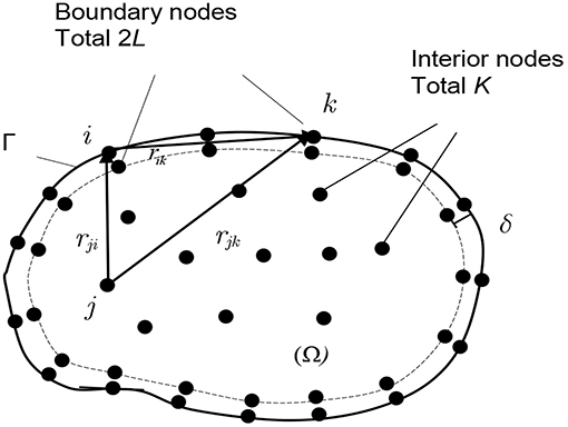
Figure 2. Boundary and domain nodal points.

Equations (16) can be directly integrated to yield

$\begin{array}{cc}u\simeq {\displaystyle \sum _{j=1}^{K+L}}{a}_j^{(1)}(t){û}_j,\nu \simeq {\displaystyle \sum _{j=1}^{K+L}}{a}_j^{(2)}(t){\widehat{\nu }}_j,w\simeq {\displaystyle \sum _{j=1}^{K+2L}}{a}_j^{(3)}(t){ŵ}_j,& (\mathrm{17a,b,c})\end{array}$

where ${û}_j(r),{\widehat{\nu }}_j(r),{ŵ}_j(r)$ are solutions of the equations

$\begin{array}{cc}{\nabla }^2{û}_j=f_j(r),{\nabla }^2{\widehat{\nu }}_j=f_j(r),{\nabla }^4{ŵ}_j=f_j(r).& (\mathrm{18a,b,c})\end{array}$

Since the functions f_j(r) depend only on the radial distance r, the solution of Equations (18) can be obtained after writing them in polar coordinates. For the 2nd order equations, we have

$\begin{array}{rc}{\nabla }^2{û}_j=\frac{1}{r}\frac{d}{dr}(r\frac{d{û}_j}{dr})=f_j(r),& (19)\end{array}$

which after integration gives

$\begin{array}{rc}{û}_j=\frac{1}{9}{f_j}^3+\frac{1}{3}{f}_j{c}^2-\frac{c^3}{3}ln(c+f_j)+G_{1}ln(r)+H_1.& (20)\end{array}$

Similarly, we have

$\begin{array}{rc}{\widehat{\nu }}_j=\frac{1}{9}{f_j}^3+\frac{1}{3}{f}_j{c}^2-\frac{c^3}{3}ln(c+f_j)+G_{2}ln(r)+H_2.& (21)\end{array}$

The regularity condition at r = 0 demands G₁ = G₂ = 0. The remaining constants H₁, H₂ together with the shape parameter c, if not arbitrarily specified, can be determined with an optimization procedure, such as to ensure the regularity of coefficients matrix (control of the condition number) and the error minimization. It has been shown that the coefficient matrix resulting from the new RBFs is always invertible (Sarra, 2006), and as a result, we take in this analysis H₁ = H₂ = 0 for convenience. Thus only c, the shape parameter is involved in the error minimization procedure (Katsikadelis, 2008a).

For the 4th order equation, one can write

$\begin{array}{rc}{\nabla }^4ŵ={\nabla }^2({\nabla }^2ŵ)=f_j.& (22)\end{array}$

Integrating Equation (22), and removing the singular terms and the terms including the arbitrary constants (Yao et al., 2010) yield

$\begin{array}{rc}{ŵ}_j=-\frac{7}{60}{c}^4{f}_j+\frac{2}{45}{c}^2{f_j}^3+\frac{1}{225}{f_j}^5+\frac{2c^2-5r^2}{60}{c}^{3}ln(c+f_j)+\frac{1}{12}{r}^2{c}^3.& (23)\end{array}$

Direct differentiation of Equations (17) obtains the derivatives of the displacements involved in the governing equations (9a,b,c).

$\begin{array}{cc}\begin{array}{c}u{,}_{ikl}\simeq {\displaystyle \sum _{j=1}^{K+L}}{a}_j^{(1)}(t){û}_j{,}_{ikl},\nu {,}_{ikl}\simeq {\displaystyle \sum _{j=1}^{K+L}}{a}_j^{(2)}(t){\widehat{\nu }}_j{,}_{ikl},\\ w{,}_{ikl}\simeq {\displaystyle \sum _{j=1}^{K+2L}}{a}_j^{(3)}(t){ŵ}_j{,}_{ikl},\end{array}& (\mathrm{24a,b,c})\end{array}$

where i, k, l stand for x, s.

Furthermore, the derivatives of the displacements with respect to time can also be obtained by direct differentiation of Equations (17). Thus we have

$\begin{array}{cc}\stackrel{°}{u}\simeq {\displaystyle \sum _{j=1}^{K+L}}{ȧ}_j^{(1)}(t){û}_j,\stackrel{°}{\nu }\simeq {\displaystyle \sum _{j=1}^{K+L}}{ȧ}_j^{(2)}(t){\widehat{\nu }}_j,ẇ\simeq {\displaystyle \sum _{j=1}^{K+2L}}{ȧ}_j^{(3)}(t){ŵ}_j,& (\mathrm{25a,b,c,})\end{array}$

$\begin{array}{cc}ü\simeq {\displaystyle \sum _{j=1}^{K+L}}{ä}_j^{(1)}(t){û}_j,\ddot{\nu }\simeq {\displaystyle \sum _{j=1}^{K+L}}{ä}_j^{(2)}(t){\widehat{\nu }}_j,ẅ\simeq {\displaystyle \sum _{j=1}^{K+2L}}{ä}_j^{(3)}(t){ŵ}_j.& (\mathrm{26a,b,c})\end{array}$

Collocating Equations (9) at the K nodal points inside Ω and the four boundary conditions, Equations (10), at the L boundary nodal points (Figure 2) using the well-known δ-technique for multiple boundaries (Yiotis and Katsikadelis, 2015a), and inserting Equations (17) and (24) to (26) in the resulting expressions, a system of ordinary differential equations is obtained, namely

$\begin{array}{rc}\text{M}\ddot{\text{a}}+\text{C}\stackrel{°}{\text{a}}+\text{K}\text{a}=\text{g},& (27)\end{array}$

where M, C, and K are known square matrices having dimension 3K+4L; g is a vector including the 3K values of the external load g(x, t) and a is the vector of the 3K+4L values of the unknown time-dependent coefficients $a_j^{(1)}(t)$, $a_j^{(2)}(t)$, $a_j^{(3)}(t)$.

Equation (27) is the semi-discretized equation of motion of the cylindrical shell with M, C, and K representing the generalized mass, damping and stiffness matrices, respectively. It can be solved numerically, using any time step integration technique to establish the time-dependent unknown coefficients. Here the method presented in Katsikadelis (2014a,b) is employed. The initial conditions of Equation (27) result from Equations (17) and (25) on the basis of Equations (11) as follows:

$\begin{array}{cc}{a}^{(1)}(0)={\widehat{u}}^{-1}{\text{g}}_1(x),{\stackrel{.}{a}}^{-1}(0)={\widehat{u}}^{-1}{h}_1(x),& (\mathrm{28a})\end{array}$

$\begin{array}{cc}{a}^{(2)}(0)={\widehat{\nu }}^{-1}{\text{g}}_2(x),{\stackrel{.}{a}}^{(2)}(0)={\widehat{\nu }}^{-1}{h}_2(x),& (\mathrm{28b})\end{array}$

$\begin{array}{cc}{a}^{(3)}(0)={\widehat{w}}^{-1}{\text{g}}_3(x),{\stackrel{.}{a}}^{(3)}(0)={\widehat{w}}^{-1}{h}_3(x).& (\mathrm{28c})\end{array}$

Once the coefficients $a_j^{(1)}(t)$, $a_j^{(2)}(t)$, $a_j^{(3)}(t)$ have been computed, the field functions u, ν, w, their derivatives, and the stress resultants can be evaluated from Equations (17), (24) to (26) and (12) to (14).

For free vibrations it is C = g(x, t) = 0 and the equation of motion, Equation (27), takes the form

$\begin{array}{rc}\text{M}\ddot{\text{a}}+\text{K}\text{a}=0,& (29)\end{array}$

while the essential boundary conditions, Equations (10), become homogeneous.

By setting

$\begin{array}{rc}\text{a}(t)=\alpha e^{i\omega t},& (30)\end{array}$

Equation (29) results in the eigenvalue problem

$\begin{array}{rc}\left[\text{K}-{\omega }^2\text{M}\right]\alpha =0,& (31)\end{array}$

which gives the eigenfrequencies ω_i and the eigenvectors α = [α⁽¹⁾, α⁽²⁾, α⁽³⁾]T, where ${\alpha }^{(1)}={\left[{\alpha }_1^{(1)},{\alpha }_2^{(1)},\dots ,{\alpha }_{K+L}^{(1)}\right]}^T$, ${\alpha }^{(2)}={\left[{\alpha }_1^{(2)},{\alpha }_2^{(2)},\dots ,{\alpha }_{K+L}^{(2)}\right]}^T$, ${\alpha }^{(3)}={\left[{\alpha }_1^{(3)},{\alpha }_2^{(3)},\dots ,{\alpha }_{K+2L}^{(3)}\right]}^T$. The elements of these vectors are the three sets of coefficients corresponding to the functions u, ν, and w, respectively. Subsequently, the mode shapes are obtained by substituting α = [α⁽¹⁾, α⁽²⁾, α⁽³⁾]T in Equations (17).

The accuracy of the approximation (9) depends heavily on c (see Equations 20-21-23). This was also verified in the problem at hand. Thus we come across to the problem of selecting a “good” value for c, that is, a value of the shape parameters that produces results of acceptable accuracy. Several methods have been suggested (Hardy, 1971; Franke, 1982; Foley, 1994; Rippa, 1999; Katsikadelis, 2009) for selecting a good value for c in 2D problems. Katsikadelis (2006, 2008b) proposed the minimization of the functional (total potential) for obtaining an optimal value for c. For the present problem, the optimal value is obtained by the search method as the value of c which yields the minimum value of the eigenfrequencies ω_i. It was observed that the optimum c giving the minimum 1st eigenfrequency differs negligibly from that yielding the higher minimum eigenfrequencies. Therefore the same optimum value of c can be used to avoid the search method for higher eigenfrequencies.

Numerical Examples

On the basis of the above analysis, a Fortran program has been written. The expressions of the derivatives involved in Equations (9) to (11) and Equations (12) to (14) have been obtained using the symbolic language MAPLE. Though the method applies to cylindrical shell of variable radius of curvature, for reasons of simplicity, the efficiency and accuracy of the developed method are demonstrated by studying the forced and free vibrations of circular cylindrical panels, (Figure 3), under different sets of boundary conditions. The NASTRAN FEM code and a model with 400 rectangular elements (Figure 4B) are used to compare the results. In all examples the employed material constants are: E = 21 × 10⁶kN/m², ν = 0.30. The results have been obtained running the relevant programs on an Intel Core 1.6 GHz with RAM 4 GB computer.

FIGURE 3

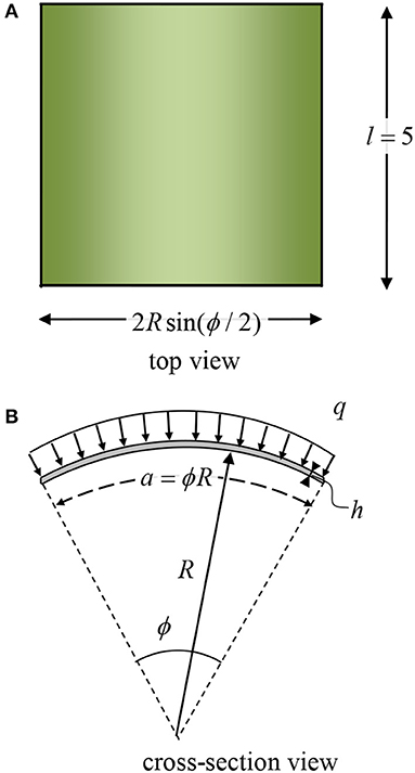
Figure 3. The circular cylindrical shell and its geometry.

FIGURE 4

Figure 4. (A) Shell collocation scheme MAEM. (B) Shell discretization FEM.

Example 1

We study the dimensionless eigenfrequency parameter ${\Omega }_f=R\omega \sqrt{(1-{\nu }^2)\rho /E}$ of a simply supported circular cylindrical shell panel with movable curved edges in the axial direction (N_x = v = w = M_x = 0 along the curved edges and u = v = w = M_s = 0 along the straight edges). The first six eigenfrequency parameters from MAEM are given in Table 1 and are compared with a FEM solution. The 1st and 2nd vibration modes for the normal displacement are shown in Figure 5, respectively. The numerical results have been obtained with the parameters L = 80, K = 361 and δ = 1.e−6 as shown in Figure 4A. The optimal value c_opt = 0.06 corresponds to the 1st mode and has also been used for the other five modes. This value is close to that obtained by the formula $c=2/\sqrt{(K+2L)=}0.088$ proposed in Ferreira et al. (2006b). The employed geometrical data are: h = 0.10 m, R = 10.00 m, l = 5.00 m, a = 5.00 m. The CPU time for the FEM solution was 10 s, while for the MAEM was 85 s. Note that the employed code has not been optimized.

TABLE 1

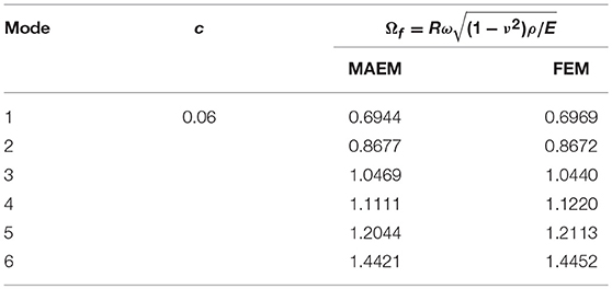
Table 1. Eigenfrequency parameters of the shell in Example 1.

FIGURE 5

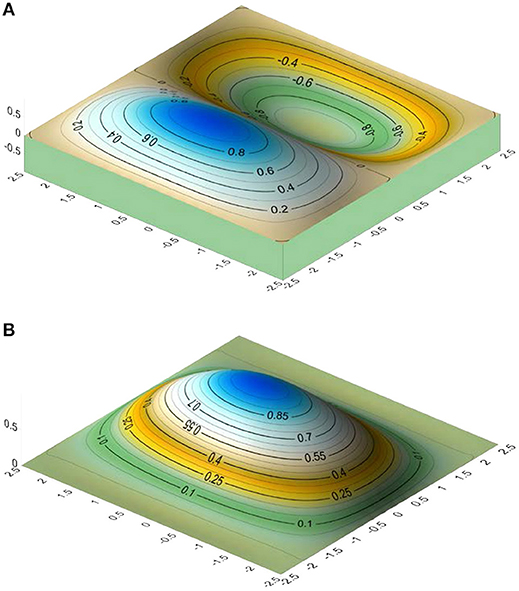
Figure 5. (A) 1st vibration mode of the shell in Example 1. (B) 2nd vibration mode of the shell in Example 1.

Example 2

In this example the same shell as in Example 1 is analyzed under the following boundary conditions: N_x = ν = w = θ_x = 0 along the curved edges and u = ν = w = θ_s = 0 along the straight edges. The same collocation points as in the Example 1 have been used. The first six eigenfrequency parameters are shown in Table 2 as compared again with those obtained from a FEM solution. The 1st and 2nd vibration modes for the normal displacement are shown in Figure 6 respectively. The value c_opt = 0.06 was employed to obtain results for the first six modes. The CPU time for the FEM solution was 10 s, while for the MAEM was 88 s.

TABLE 2

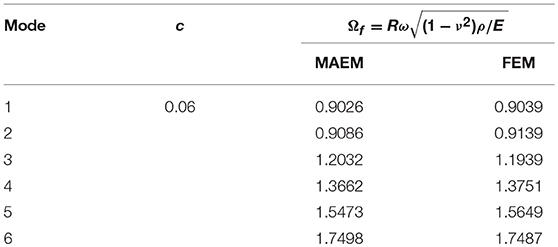
Table 2. Eigenfrequency parameters of the shell in Example 2.

FIGURE 6

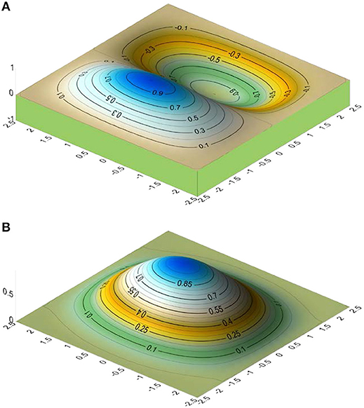
Figure 6. (A) 1st vibration mode of the shell in Example 2. (B) 2nd vibration mode of the shell in Example 2.

Example 3

In this example, a cylindrical shell panel with geometrical data R = 9.896 m, l = 4.949 m, a = 5.00 m is analyzed. Two cases with regard to the thickness have been considered: (a) 2Rsin(ϕ/2)/h = 100 and (b)2Rsin(ϕ/2)/h = 20. All edges are clamped, i.e., u = ν = w = θ_x = 0 along the curved edges and u = ν = w = θ_s = 0 along the straight edges. The numerical results have been obtained with L = 80, K = 361 randomly distributed as shown in Figure 7, that is using an irregular distribution, and δ = 1.e−6. In both cases, the search method resulted c_opt = 0.05. The first eight eigenfrequency parameters are shown in Tables 3, 4 as compared with those obtained from an analytical solution (Lim and Liew, 1994). The 1st and 2nd vibration modes for the normal displacement are shown in Figure 8 for case (a) and in Figure 9 for case (b), respectively. These figures show that that the vibration modes are influenced by the thickness of the shell, which is verified in (Webster, 1968; Lim and Liew, 1994).

FIGURE 7

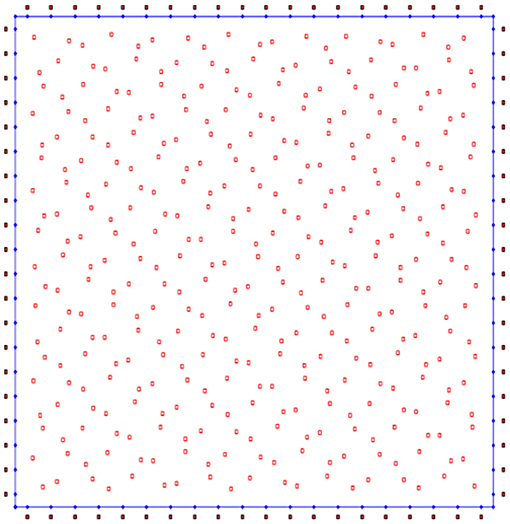
Figure 7. Shell irregular collocation scheme: MAEM.

TABLE 3

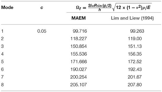
Table 3. Eigenfrequency parameters of the shell in Example 3: case (a).

TABLE 4

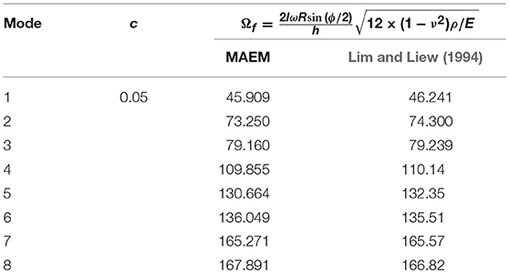
Table 4. Eigenfrequency parameters of the shell in Example 3: case (b).

FIGURE 8

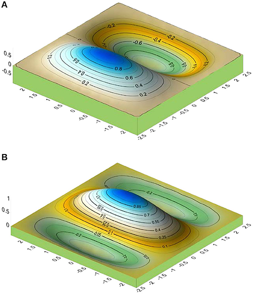
Figure 8. (A) 1st vibration mode of the shell in Example 3-case (a). (B) 2nd vibration mode of the shell in Example 3-case (a).

FIGURE 9

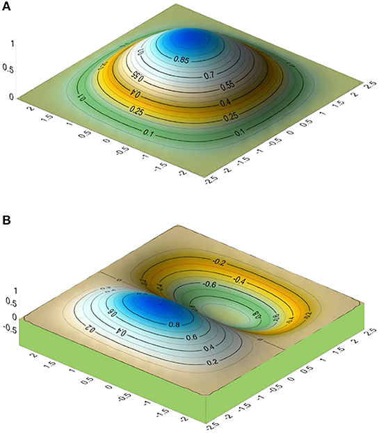
Figure 9. (A) 1st vibration mode of the shell in Example 3-case (b). (B) 2nd vibration mode of the shell in Example 3-case (b).

Example 4

In this example, the forced vibrations of a simply supported circular cylindrical shell panel (u = ν = w = M_x = 0 along the curved edges and u = ν = w = M_s = 0 along the straight edges) with zero initial conditions ($u(\mathrm{\text{x}},0)=\stackrel{°}{u}(\mathrm{\text{x}},0)=\nu (\mathrm{\text{x}},0)=\stackrel{°}{\nu }(\mathrm{\text{x}},0)=w(\mathrm{\text{x}},0)=ẇ(\mathrm{\text{x}},0)=0$) has been studied. Its geometrical data are those of Example 1. The applied load is the normal pressure given by $q_z=sin(t)kN/m^2$. The mass density is ρ = 2.446kNm⁻⁴sec². The numerical results have been obtained with L = 80, K = 361 distributed as shown in Figure 4A and δ = 1.e−6. The employed optimal value is c_opt = 0.06. The time history of the normal displacement w, the bending moment M_s and the membrane force N_s at the center of the shell are shown in Figure 10 as compared with those obtained by a FEM solution. The CPU time for the FEM solution was 40 s, while for the MAEM was 325 s.

FIGURE 10

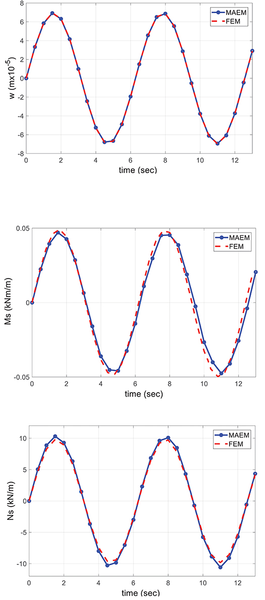
Figure 10. Time history of the normal displacement w, bending moment M_s, and membrane force Ns at the center of the shell in Example 4.

Conclusions

The Meshless Analog Equation Method, a truly meshless method, has been applied to the dynamic analysis of thin cylindrical shell panels in the present study. MAEM is based on the principle of the analog equation, converting the original equations into three substitute equations, two Poisson's and one biharmonic, which are solved using a meshless method. The use of integrated MQ-RBFs to approximate the fictitious sources allows the approximation of the sought solutions by new RBFs, which approximate both the solution and its derivatives accurately. This way the strong formulation of the problem avoids the drawbacks inherent in the conventional MQ-RBFs, while maintaining all the advantages of a truly mess-free method. A method is presented to obtain optimum values for the shape parameter, eliminating the uncertainty in its choice. It was observed that the optimum value of the shape parameter for the 1st mode differs negligibly from those of higher modes and therefore the same value can be used to obtain the eigenfrequencies of higher modes. The solution algorithm is straightforward and quite reasonably easy to program. The numerical examples presented demonstrate the efficiency and accuracy of the proposed method and show that MAEM can be used as an efficient solver for challenging problems in engineering analysis.

Author Contributions

AY has implemented the MAEM (Meshless Analog Equation Method) for the solution of problems governing by fourth order differential equations (plates-shells etc.). JK has invented the AEM (Analog Equation Method), which is a general method for the solution of various engineering problems.

Conflict of Interest Statement

The authors declare that the research was conducted in the absence of any commercial or financial relationships that could be construed as a potential conflict of interest.

The reviewer AC declared a shared affiliation, with no collaboration, with the authors to the handling editor at time of review.

References

Beskos, D. E. (1991). “Static and dynamic analysis of shells,” in Boundary Element Analysis of Plates and Shells, ed D. E. Beskos (Berlin: Springer-Verlag), 93–140.

Google Scholar

Cheng, A. H. D., Golbeg, M. A., Kansa, E. J., and Zammito, G. (2003). Exponential1 convergence and h-c multiquadric collocation method for partial differential equations. Numerical Methods Partial Differential Equations 19, 571–594. doi: 10.1002/num.10062

CrossRef Full Text | Google Scholar

Dinis, L. M. J. S., Natal Jorge, R. M., and Belinha, J. (2011). A natural neighbour meshless method with a 3D shell-like approach in the dynamic analysis of thin 3D structures. Thin-Walled Structures 49, 185–196. doi: 10.1016/j.tws.2010.09.023

CrossRef Full Text | Google Scholar

Ferreira, A. J. M., Roque, C. M. C., and Jorge, R. M. M. (2006a). Modelling cross-ply laminated elastic shells by a higher-order theory and multiquadrics. Comput. Struct. 84, 1288–99. doi: 10.1016/j.compstruc.2006.01.021

CrossRef Full Text | Google Scholar

Ferreira, A. J. M., Roque, C. M. C., and Jorge, R. M. M. (2006b). Static and free vibration analysis of composite shells by radial basis functions. Eng. Anal. Bound.Elements 30, 719–733. doi: 10.1016/j.enganabound.2006.05.002

CrossRef Full Text | Google Scholar

Ferreira, A. J. M., Roque, C. M. C., and Martins, P. A. L. S. (2005). Analysis of thin isotropic rectangular and circular plates with multiquadrics. Strength Mater. 37, 163–173. doi: 10.1007/s11223-005-0029-7

CrossRef Full Text | Google Scholar

Flügge, W. (1962). Stresses in Shells. Berlin: Springer-Verlag.

Google Scholar

Foley, T. A. (1994). Near optimal parameter selection for multiquadric interpolation. J. Appl. Sci. Comput. 1, 54–69.

Google Scholar

Franke, R. (1982). Scattered data interpolation: tests of some methods. Math. Comput. 38, 181–200.

Google Scholar

Hardy, R. L. (1971). Multiquadric equations of topography and other irregular surfaces. J. Geophys. Res. 76, 1905–1915. doi: 10.1029/JB076i008p01905

CrossRef Full Text | Google Scholar

Jang, S. K., Bert, C. W., and Striz, A. G. (1989). Application of differential quadrature to static analysis of structural components. Int. J. Num. Methods Eng. 28, 561–577. doi: 10.1002/nme.1620280306

CrossRef Full Text | Google Scholar

Kansa, E. J. (2005). “Highly accurate methods for solving elliptic partial differential equations,” in Boundary Elements XXVII, eds C. A. Brebbia, E. Divo, and D. Poljak (Southampton: WIT Press), 5–15.

Google Scholar

Katsikadelis, J. T. (2002). The analog equation method. A boundary-only integral equation method for nonlinear static and dynamic problems in general bodies. Int. J. Theor. Appl. Mech. Arch. Appl. Mech. 27, 13–38. doi: 10.2298/TAM0227013K

CrossRef Full Text

Katsikadelis, J. T. (2006). “The meshless analog equation method. A new highly accurate truly mesh-free method for solving partial differential equations,” in Boundary Elements and Other Mesh Reduction Methods XXVIII, eds C. A. Brebbia and J. T. Katsikadelis (Southampton: WIT Press), 13–22. doi: 10.2495/BE06002

CrossRef Full Text | Google Scholar

Katsikadelis, J. T. (2008a). A generalized Ritz method for partial differential equations in domains of arbitrary geometry using global shape functions. Eng. Anal. Bound. Elem. 32, 353–367. doi: 10.1016/j.enganabound.2007.09.001

CrossRef Full Text | Google Scholar

Katsikadelis, J. T. (2008b). The 2D elastostatic problem in inhomogeneous anisotropic bodies by the meshless analog equation method MAEM. Eng. Anal. Bound. Elem.32, 997–1005. doi: 10.1016/j.enganabound.2007.10.016

CrossRef Full Text | Google Scholar

Katsikadelis, J. T. (2009). The meshless analog equation method: I. Solution of elliptic partial differential equations. Arch. Appl. Mech. 79, 557–578. doi: 10.1007/s00419-008-0294-6

CrossRef Full Text

Katsikadelis, J. T. (2014a). A new direct time integration method for the equations of motion in structural dynamics. Zeitschrift Angewandte Math Mech. 94, 757–774. doi: 10.1002/zamm.201200245

CrossRef Full Text | Google Scholar

Katsikadelis, J. T. (2014b). Boundary Element Method for Plate Analysis. Oxford, UK: Academic Press; Elsevier.

Google Scholar

Katsikadelis, J. T. (2016). The Boundary Element Method for Engineers and Scientists, 2nd Edn. Oxford, UK: Academic Press; Elsevier.

Google Scholar

Katsikadelis, J. T., and Platanidi, J. G. (2007). “3D analysis of thick shells by the meshless analog equation method,” in Proceedings of the 1st International Congress of Serbian Society of Mechanics, (Kopaonik), 475–484.

Google Scholar

Kraus, H. (1967). Thin Elastic Shells. An Introduction to the Theoretical Foundations and the Analysis of Their Static and Dynamic Behavior. New York, NY; London; Sydney: John Wiley and Sons.

Google Scholar

Lee, S. J., and Han, S. E. (2001). Free-vibration analysis of plates and shells with a nine-node assumed natural degenerated shell element. J. Sound Vibr. 241, 605–633. doi: 10.1006/jsvi.2000.3313

CrossRef Full Text | Google Scholar

Leissa, A. W. (1973). Vibrations of Shells, Scientific and Technical Information Office. Washington, DC: NASA.

Google Scholar

Lim, C. W., and Liew, K. M. (1994). A pb-2 Ritz formulation for flexural vibration of shallow cylindrical shells of rectangular planform. J. Sound. Vibr. 173, 343–375. doi: 10.1006/jsvi.1994.1235

CrossRef Full Text | Google Scholar

Liu, G. R. (2002). Meshfree Methods: Moving Beyond the Finite Element Method. New York, NY: CRC Press.

Google Scholar

Liu, G. R., and Gu, Y. T. (2005). An Introduction to Meshfree Methods and Their Programming. Dordrecht: Springer.

Google Scholar

Liu, L., Chua, L. P., and Ghista, D. N. (2006). Element free Galerkin method for static and dynamic analysis of spatial shell structures. J. Sound Vibr. 295, 388–406. doi: 10.1016/j.jsv.2006.01.015

CrossRef Full Text | Google Scholar

Love, A. E. H. (1944). A Treatise on the Mathematical Theory of Elasticity, 4th Edn. New York, NY: Dover Pub Inc.

Google Scholar

Nguyen, V. P., Rabczuk, T., Bordas, S., and Duflot, M. (2008). Meshless methods: a review and computer implementation aspects. Math. Comput Simul. 79, 763–813. doi: 10.1016/j.matcom.2008.01.003

CrossRef Full Text | Google Scholar

Pilafkan, R., Folkow, P. D., Darvizeh, M., and Darvizeh, A. (2013). Three dimensional frequency analysis of bidirectional graded thick cylindrical shells using a radial point interpolation method (RPIM). Eur. J. Mech. A/Solids 39, 26–34. doi: 10.1016/j.euromechsol.2012.09.014

CrossRef Full Text | Google Scholar

Rippa, S. (1999). An algorithm for selecting a good value for the parameter c in radial basis function approximation. Adv. Comput. Math. 11, 193–210. doi: 10.1023/A:1018975909870

CrossRef Full Text | Google Scholar

Roque, C. M. C., Ferreira, A. J. M., Neves, A. N. A., Fasshauer, G. E., Soares, C. M. M., and Jorge, R. M. N. (2010). Dynamic analysis of functionally graded plates and shells by radial basis functions. Mech. Adv. Mater. Struct. 17, 636–652. doi: 10.1080/15376494.2010.518932

CrossRef Full Text | Google Scholar

Sarra, S. A. (2006). Integrated multiquadric radial basis function approximation methods. Comput. Math. Appl. 51, 1283–1296. doi: 10.1016/j.camwa.2006.04.014

CrossRef Full Text | Google Scholar

Webster, J. J. (1968). Free vibrations of rectangular curved panels. Int. J. Mech. Sci. 10, 571–582. doi: 10.1016/0020-7403(68)90058-1

CrossRef Full Text | Google Scholar

Yao, G., Tsai, C. H., and Chen, W. (2010). The comparison of three meshless methods using radial basis functions for solving fourth-order partial differential equations. Eng. Analysis Bound. Elem. 34, 625–631. doi: 10.1016/j.enganabound.2010.03.004

CrossRef Full Text | Google Scholar

Yiotis, A. J., and Katsikadelis, J. T. (2000). Static and dynamic analysis of shell panels using the analog equation method. Comput. Model. Eng. Sci. 2, 95–103. doi: 10.3970/cmes.2000.001.255

CrossRef Full Text | Google Scholar

Yiotis, A. J., and Katsikadelis, J. T. (2008). “The Meshless Analog Equation Method for the solution of plate problems,” in Proceedings of the 6th GRACM International Congress on Computational Mechanics (Thessaloniki).

Google Scholar

Yiotis, A. J., and Katsikadelis, J. T. (2013). Analysis of cylindrical shell panels. A Meshless Solution. Eng. Anal. Bound. Elem. 37, 928–935. doi: 10.1016/j.enganabound.2013.03.005

CrossRef Full Text

Yiotis, A. J., and Katsikadelis, J. T. (2015a). Buckling of cylindrical shell panels. A MAEM solution. Arch. Appl. Mech. 85, 1545–1557. doi: 10.1007/s00419-014-0944-9

CrossRef Full Text | Google Scholar

Yiotis, A. J., and Katsikadelis, J. T. (2015b). “The dynamic analysis of cylindrical shell panels. A MAEM solution,” in Book of Abstracts of the 8th GRACM International Congress on Computational Mechanics, July 12–15, eds N. Pelekasis and E. G. Stavroulakis (Volos), 147.

Google Scholar

Zhao, X., Lee, Y. Y., and Liew, K. M. (2009). Thermoelastic and vibration analysis of functionally graded cylindrical shells. Int. J. Mech. Sci. 51, 694–707. doi: 10.1016/j.ijmecsci.2009.08.001

CrossRef Full Text | Google Scholar