Phenomenological Model of Rubber Bearings With Variable Axial Loading

Introduction

Passive, anti-seismic, systems have already been used to protect more than 20,000 structures among bridges and buildings, both of existing and of new construction, in more than 30 countries. Among others protection systems, the seismic isolation ones are recognized as the most effective in terms of structural integrity due to reduction of the absolute accelerations, interstory drifts, and minimization of the “panic” effect for the occupants. Although their adoption is still limited, with respect to the protection of strategic buildings, seismic base isolation is likely to become a widespread solution in the design of structures and facilities that require superior performances and need to retain functionality after an earthquake event (Basu et al., 2014).

Base isolation is usually implemented with reference to the national and international standards, resorting to one of two broad classes of isolation devices: flat or curved surface sliders and elastomeric isolators. The response of both these families of base isolation devices depend, for different reasons, on the value of the axial force acting on the device. This dependence, in the case of near field earthquakes characterized by vertical components with the same intensity of the horizontal ones, has been recognized peculiar for base isolated structures to such an extent that base isolation protection has proved to be rather ineffective (Bhandari et al., 2017). Therefore, besides being of interest on its own, recognizing how coupled vertical-horizontal response affects the isolation performance has important practical consequences. In this light, this work is aimed at studying and developing an innovative model able to include such coupled response within a consolidated analytical modeling approach for elastomeric devices (Domaneschi et al., 2015). It is the differential hysteretic formulation by Abe et al. (2004a,b) for laminated natural, high damping (HDRB) and lead-core (LRB) rubber bearings under biaxial and tri-axial loading conditions (constant axial force and respectively single or both horizontal components of displacement). Such formulation has been proved effective in reproducing the experimental physical behavior of rubber bearings including several effects (e.g., scragging and Mullins' effects—stiffness and damping degradation) and performs satisfactorily for complex seismic structural analyses (Perotti et al., 2013). However, in its current formulation, it reproduce the device response at a fixed value of the axial load only.

In the literature several other models for elastomeric devices are available that include coupling with the axial load. Among these, Ryan et al. (2005) proposed an innovative formulation to the problem of the influence of the axial load variation on the isolator horizontal stiffness and yielding strength. Their model is a non-linear extension of a two-spring model developed from the linear stability theory of multilayer bearings (Kelly, 1997). The following considerations has been underlined for both HDRB and LRB: (i) the lateral stiffness decreases with the increasing axial load; (ii) the lateral yield strength decreases with decreasing axial load (LRB only); (iii) the vertical stiffness decreases with increasing lateral deformation. The proposed solutions, although an improvement, are reported by the Authors as an incomplete representation of the experimental response (e.g., no hardening appears in the simulated results).

Yamamoto et al. (2009) also proposed a two-dimensional model for the numerical simulation of seismic isolation bearings including the influence of axial load. Such model is inspired by the Kikuchi and Aiken (1997) formulation and consists in an analytical approach comprising several shear and axial springs (these last working in parallel), having properties which vary with the vertical load. In particular, the axial effect is captured by the material non-linearity formulation of the axial springs and by the transversal geometric non-linearity of the shear stiffness. The effect of the coupled loading components on the device stiffening and buckling response is also studied, driven by axial stresses under large deformations. A three dimensional development of this model has been reported in Kikuchi et al. (2010). However, no evaluation of the performance is given under three dimensional loading paths and seismic loads. Furthermore, the formulation that adopts several non-linear springs can become numerically expensive in the case of structures that are base isolated with a substantial number of isolation devices.

Similarly, in the literature there are research works focused on the effect of the vertical and horizontal loading on the critical buckling loading capacity of rubber bearings. Experimental results are employed for developing numerical approaches based on mechanical models comprising linear and rotational springs in different directions.

Kumar et al. (2014) implemented a new mechanical formulation in OpenSees code as a new three-dimensional finite user element, arranging linear and rotational springs. Numerical results compare well with the experimental data for behavior in tension. The critical buckling load capacity at extreme loading is correctly predicted, decreasing linearly with the lateral displacement and the related overlap area. The model, however, doesn't seem to include provisions for the strain hardening behavior highlighted in the testing of physical devices at large shear strain values.

Han and Warn (2015) studied the unstable equilibrium of elastomeric bearings through a mechanical model similar to the one by Kelly (1997), consisting in series of vertical springs and a simple bilinear constitutive relationship to represent the rotational behavior of elastomeric bearings. The critical behavior under simultaneous vertical compressive load and lateral displacement is assessed with accuracy, without relying on experimentally calibrated parameters. Since several hyperelastic springs appear inside this model, a comment similar as for the model of Kikuchi et al. (2010) arises.

Vemuru et al. (2003) studied the coupled horizontal–vertical behavior of elastomeric bearings (with constant vertical load) by analytically developing a mechanical model. They observe that the coupled behavior of the bearings under dynamic loading differs considerably from that observed under quasi-static conditions.

The above-mentioned literature works propose several numerical approaches for including the coupled axial force-shear response of rubber bearings up to the buckling load capacity of the device. All the reported analytical (non-differential) models are developed with reference to experimental results and essentially consist in a, sometimes large, series of non-linear springs arranged with different connection schemes. Despite the effectiveness each of them shows within the specific range of application, the Abe et al. (2004a,b) model remains the reference for its compactness and satisfactory representation of the experimental response for both cyclic and seismic loading at small and large value of relative displacement between the device ends.

The present paper is focused on modeling the response of rubber bearings, extending the model by Abe et al. (2004a,b) to variable axial loading. Suitable laboratory experimental tests, available in the literature (Yamamoto et al., 2009), represent the target for illustrating the proposed numerical approach. This work is limited to the bidirectional formulation (vertical-horizontal) as the general three-dimensional formulation is out of the scope of this study. However, consistently with the original formulation by Abe et al. (2004a,b), from which it is inspired, the generalization of the bidirectional model herein proposed can be obtained by following the methodology there presented. The next section is devoted to the presentation of the cycling loading experimental results from the literature and the reference rubber bearing specimen. Subsequently, the original phenomenological model that will be extended is presented, then the identification of the model parameters is described. Several strategies for the parameters identification are implemented and the best set in terms of matching with the experimental target is defined as the “superset.” The consequences stemming from the proposed enhancement of the bearing model and the comparison with the original standard model from the literature are finally presented within a structural application relative to the seismic response of a base isolated nuclear building.

Reference Specimen and Laboratory Tests

Cyclic shear tests of lead–rubber bearings were conducted by Yamamoto et al. (2009) to identify the mechanical characteristics of lead-rubber bearings under large deformations at different values of constant axial load. The tests deal with a device having 24 layers of 2.0 mm thick rubber, and a 250 mm diameter (see Figure 1). Thus, the rubber layer shape factor (ratio between the steel layer area and the lateral surface of a single rubber layer) results S₁ = 31.3 and the second shape factor (ratio of the device diameter and the total thickness of the rubber layers) S₂ = 5.2. The bearing embeds a 50.0 mm diameter lead plug (Table 1).

FIGURE 1

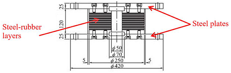
Figure 1. The tested bearing [mm].

TABLE 1

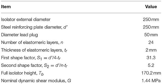
Table 1. Characteristics of the tested isolator.

The cyclic shear tests consisted in applying a sinusoidal horizontal displacement with four cycles of loading at the increasing shear strain amplitudes of 50, 100, 200, 300, and 400 %, while the vertical load applied to the bearing was maintained constant. The tests were repeated at compressive stresses of σ = 0, 5, 10, 20, and 30 MPa.

At the lowest axial stresses (σ = 0, 5, and 10 MPa), the hysteresis loops obtained from the cyclic shear tests exhibited (shear) stiffening behavior beyond the shear strain value of 300% and a deterioration of horizontal stiffness is seen for higher compression stresses (σ = 20 and 30 MPa). Furthermore, significant negative stiffness appeared at 30 MPa axial compressive loading.

Reference and Enhanced Isolator Model

The reference isolator model here adopted as a starting point for developing a new procedure to model isolation devices that includes the effects of the axial force is the one (Abe et al., 2004a,b). In that model the restoring force F is obtained as the sum of three contributions (Figure 2), superimposing a force component coming from an elastic non-linear spring (F₁), the hysteretic force in an elastic-plastic spring (F₂) and, finally, a second elastic non-linear force for an hardening contribution (F₃). Such components are defined by the following equations.

$\begin{array}{lll}F=F_1+F_2+F_3& & (1)\end{array}$

$\begin{array}{l}{F}_1=K_1\left\{\beta +(1-\beta )\exp (-\frac{U_{\max }}{\alpha })\right\}U\\ \text{\hspace{0.17em}\hspace{0.17em}\hspace{0.17em}\hspace{0.17em}\hspace{0.17em}\hspace{0.17em}\hspace{0.17em}\hspace{0.17em}\hspace{0.17em}\hspace{0.17em}}+a\left[1-\exp (-b\left|U\right|)\right]\text{sgn}(U)& & (2)\end{array}$

$\begin{array}{ll}{U}_{max}=\text{max}(\left|\mathit{\text{U(s)}}\right|),0<s<t& (3)\end{array}$

$\begin{array}{ll}{\dot{F}}_2=\frac{Y_t}{U_t}\left\{\dot{U}-\left|\dot{U}\right|{\left|\frac{F_2}{Y_t}\right|}^n\text{sgn}(\frac{F_2}{Y_t})\right\}& (4)\end{array}$

$\begin{array}{ll}{Y}_t=Y_0(1+{\left|\frac{U}{U_H}\right|}^p)& (5)\end{array}$

$\begin{array}{ll}{U}_t=U_0(1+\frac{U_{\text{max}}}{U_S})& (6)\end{array}$

$\begin{array}{ll}{F}_3=K_2{\left|\frac{U}{U_H}\right|}^{r}U& (7)\end{array}$

FIGURE 2

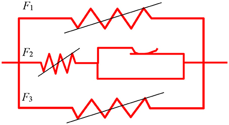
Figure 2. Schematic representation of the Abe et al. (2004a,b) model.

In the previous equations U denotes the horizontal relative displacement across the isolator, F the total restoring force of the model, F_i the internal force of each spring. K₁ is the initial stiffness of the non-linear elastic spring, constants α e β required parameters for controlling the evolution of the stiffness degradation, a the force value of the non-linear elastic behaviors in the small strain range and b a parameter that controls the evolution of the non-linear elastic behaviors in the small strain range. Y_t is the yielding force and U_t the corresponding displacement of the elastic-plastic spring: both include the modeling of the increase of the hysteresis loops area through the parameters Y₀—the initial yielding force, U_H—displacement where the hardening starts, U₀—initial yielding displacement, U_S—constant that controls the degradation of the elastic stiffness of the elastoplastic spring, p—constant that prescribes the curve of the hardening. The behavior of the third non-linear elastic spring delivering the forces listed in F₃, called the hardening spring, depends on the parameters K₂ (constant that describes the contribution of the hardening spring to the other springs) and r (parameter that prescribes the curve of the hardening). This spring, working in parallel to the others, expresses the increase of the tangent stiffness at large deformations. More details on the model parameters and how they affect the behavior of springs (F₁, F₂, F₃) are reported in the original work by Abe et al. (2004a,b) and in the work by Perotti et al. (2013).

In the Abe et al. model the vertical response of the device is assumed as uncoupled from the horizontal response. However, it has been demonstrated how the horizontal response is affected by the value of the vertical force carried by the device, arriving up to buckling phenomena (Yamamoto et al., 2009; Han and Warn, 2015).

For taking into account the coupled vertical and horizontal response of the device, the original standard model has been modified. At first, the parameters of the Abe et al. model have been identified, for the different values of the axial force corresponding to compressive stresses of σ = 0, 5, 10, 20, and 30 MPa respectively, on the sample isolator tested by Yamamoto et al. (2009). The identified values have been, then, used within an interpolation procedure in computing the numerical response of the device under variable seismic vertical-horizontal loading as it will be explained in the following. Therefore, the parameters dependency on axial loading is embedded in the model formulation such that at any step of a time history analysis the parameters are updated. The next section is devoted to the identification and optimization procedures for estimating the model parameters.

Identification of the Model Parameters

The target of the optimization procedure is represented by the cyclic shear tests under large deformations, and at different axial loads (0, 5, 10, 20, 30 MPa), of lead–rubber isolators as described in the research paper by Yamamoto et al. (2009). The optimization procedures herein employed are: (a) the human-driven one which is based on the user critical assessment, (b) the Pattern Search one (Dolan et al., 2018) and, (c), the Genetic Algorithm one [tournament selection (Miller and Goldberg, 1995)]. In the first case the choice of parameters to be used is essentially heuristic, in the last two the MATLAB code implementation is used (MATLAB, 2013).

For each level of axial compression stress, and for each selected optimization procedure, a different set of the parameters has been identified coherently with the original Abe et al. model (Abe et al., 2004a,b). When automatic optimization procedures have been employed, namely the Pattern Search and the Genetic algorithm, the parameters set is found by minimizing the root mean square error (RMSE) between the cyclic experimental and numerical response to coupled vertical—horizontal loading. Conversely, when the Human-driven procedure is considered, a local sensitivity analysis and knowledge based decision allows the user to define the parameters set. The local sensitivity analysis belongs to one-at-a-time (OAT) techniques that analyze the effect of one parameter on the output at a time, keeping the other parameters fixed. They are used in particular when there are many parameters, to explore only a small fraction of the design space.

It is worth underlining how not all the Abe et al. original model parameters highlighted essential variation: the values for a number of them can be kept fixed, depending on the selected optimization procedure. They are reported in bold in Tables 2–4 and discussed in detail in the next sub-sections. For the automatic optimization procedures, the following upper and lower bounds are considered: β [0.000001,1], A [0.1,25], N [0.1,1], Y₀ [1,30], U_H [10,150], p [0.1,5], U_S [10,200], K₂ [−0.5,0.5], r [0,4].

TABLE 2

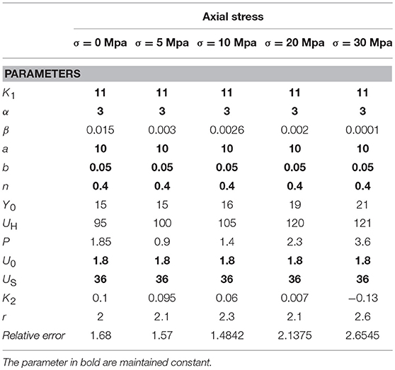
Table 2. Human-driven method: identified parameters.

As the identification process is completed, a super-set of optimal parameters is finally defined as the one corresponding, for each value of the axial stress, to the minimum of the relative error function among the identification procedures herein considered.

The function modeling the dependence on the compressive axial stresses of each model parameter of the Abe et al. model, is defined in a purely mathematical way (no attempt is herein made to relate it to physical aspects of the isolator response) according to the following procedure:

a) The form of functional dependence on the value of the axial force is assumed for each parameter of the Abe et al. model.

b) If the functional dependence form includes any coefficient, these are identified by minimizing the Mean Squared Error (MSE) in L₂ norm:

$\begin{array}{ll}MSE=\sqrt{{\displaystyle {\sum }_{i=0}^5{\left(y\left({\sigma }_i\right)-paramete{r}_i\right))}^2}}& (8)\end{array}$

where σ_i is one of the considered values of axial stress, y(σ_i) is the fitting law evaluated at axial stress σ_i, while parameter_i is the value of the Abe et al model parameter as identified from the test at constant axial stress σ = σ_i.

The next sections are devoted to the description of the optimization procedures, to the presentation of the results, to a discussion of the identification procedures and to the definition of an optimal “superset” with the corresponding fitting laws.

Human-Driven Identification

Table 2 summarizes all the identified parameters (in bold are highlighted the ones that yielded a fixed value). Last row reports the Relative Error as the ratio between the L₂ norm of the differences between the model reaction forces and the experimental ones, and the maximum reaction force in the experimental cycles. It is defined as:

$\begin{array}{ll}RelativeError=\frac{\sqrt{{\displaystyle {\sum }_{i=0}^n{(F_{model}\left(u_i,\vartheta \right)-F(u_i))}^2}}}{F_{\max }}& (9)\end{array}$

Where n is the number of the experimental and the model force values, ϑ is the model parameters vector. Figure 3 depicts the comparison between the experimental responses of the lead-rubber bearing in Yamamoto et al. (2009) and the numerical output from the Abe et al. model. Parameters in Table 2 have been used.

FIGURE 3

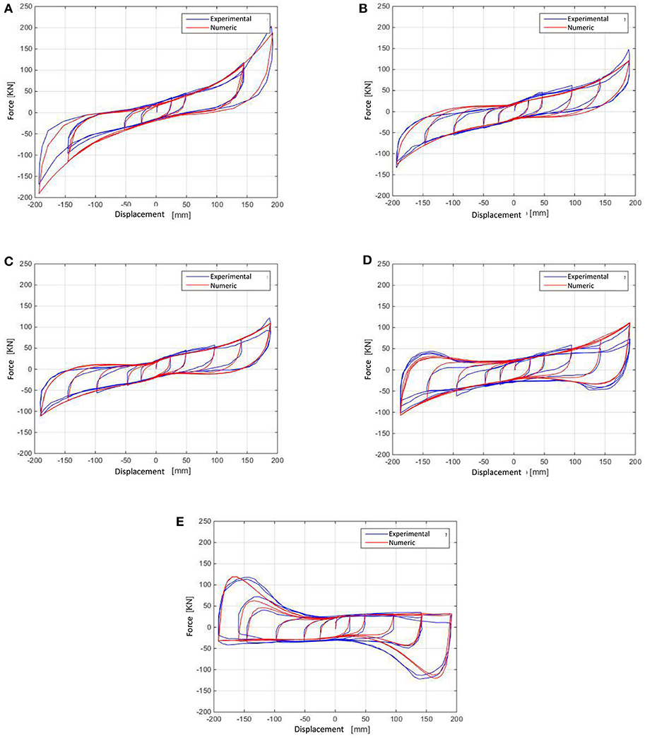
Figure 3. Human-driven method: cyclic shear test of the tested isolator (50, 100, 200, 300, and 400% deformations for compression stresses of 0 MPa (A), 5 MPa (B), 10 MPa (C), 20 MPa (D), 30 MPa (E). Comparison between model (parameters in Table 2) and experimental results.

Device #1 time histories of the axial force and relative displacement are depicted in Figures 8, 9. The simulation of the device response for the combined displacement-axial force time histories is depicted in Figure 10. About Device #2, the time histories for axial force and relative displacement are depicted in Figures 11, 12, while the simulation of the device response for the combined loading condition is depicted in Figure 13.

Focusing on Table 2, several parameters increase or decrease their value when the axial compression stresses increases. It is however interesting to note as the parameters related to the non-linear elastic behavior for deformations in the range [0, 50%] remain constant, owing to the reasonably constant response in the same range of the devices at all the compression stress values. On the contrary, for the early yielding force and the ratio between the initial and the completely degraded non-linear elastic stiffness variations are expected, as Table 2 confirms. Focusing on the parameters of the F₂ component, the yielding displacement U₀ can be considered essentially constant while the corresponding force Y₀ slightly increases with σ. Owing to the fact that the transition from the non-linear elastic branch to the plastic one is essentially constant at the increasing of compression stresses, the parameter n does not show variations. The stiffness degradation parameter U_s, related to the elastic-plastic spring, is also assumed essentially constant by observing how the unloading branches are reasonably parallel.

On the contrary, the parameter β that expresses the ratio between the completely degraded stiffness and K₁ (this one essentially constant) decreases with the compression stresses consistently with the experienced horizontal stiffness reduction in the rubber bearings at the increase of the axial compression. Consistently to this aspect, also the early hardening displacement U_H increases, while the hardening stiffness K₂ decreases. The amplification of the hysteretic cycles at increased compression stresses is related to the variation of the hardening shape related parameters (p and r).

Pattern Search Automatic Identification Procedure

The Pattern Search optimization method numerically identifies the minimum value of a function without explicitly knowing its derivatives. This method is generally useful for non-differentiable functions, or when evaluation of the exact derivative is computationally expensive (see also MATLAB, 2013). This is the case of the Abe et al. formulation, in particular for the F₂ component for which the gradient is not easily defined. At each optimization step the Pattern Search method designs a mesh of possible alternative points associated to specific searching directions. If the objective function (deviation between experimental and model reaction forces, corresponding to the prescribed displacement history) is reduced at a certain point of the mesh, with respect to the previous evaluations, that point becomes the new current one for the next optimization step. The procedure is completed as the mesh dimension becomes lower than a certain very small limit, as fixed by the user (relative error = 0.001%) (MATLAB, 2013).

The Human-driven procedure allowed through a sensitivity analysis to identify a subset of parameters, which can be assumed as constant. The same have been considered as constant also in the Pattern Search automatic procedure, apart for U_s and a. The first can improve the match of the unloading branches between experimental and numerical cycles, the second at the end of the non-linear-elastic phase. Table 3 summarizes the parameters of the Abe et al. model found with the Pattern Search method (in bold are highlighted the ones for which a fixed value is assumed) while Figure 4 depicts the comparison between the experimental responses of the lead-rubber bearing with the numerical output.

TABLE 3

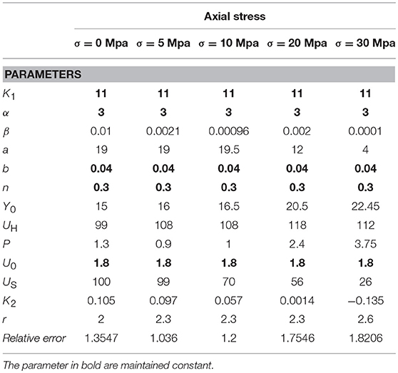
Table 3. Pattern search method: identified parameters.

FIGURE 4

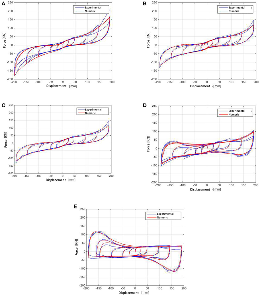
Figure 4. Pattern Search method: cyclic shear test of the tested isolator (50, 100, 200, 300, and 400% deformations for compression stresses of 0 MPa (A), 5 MPa (B), 10 MPa (C), 20MPa (D), 30MPa (E). Comparison between model (parameters in Table 3) and experimental results.

Genetic Algorithm Automatic Identification Procedure

Among the optimization procedures which do not require evaluation of the optimizing function's gradient, the Genetic Algorithms one play a significant role owing to its effectiveness in complex problem. Indeed, the procedures are extensively applied to industrial problems. Within the Genetic Algorithm Toolbox in MATLAB (2013) the Selection Tournament procedure, in particular, has been adopted (Miller and Goldberg, 1995). This procedure allows to select the optimal set in several rounds of a virtual tournament, where the “winners,” called the mating pool, create the population of the next generation of individuals. These last are then involved in a new selection process, up to when the optimal solution is reached. To overcome possible local minima, new extents of the domain are then explored through assuming that a fixed fraction of the population is subject to a random genetic mutation of its properties (fraction = 0.9). The default options of the genetic algorithm function in MATLAB (2013) have been used for the adopted population, the crossover function and the mutation operator.

The set of the Abe et al. model parameters coming from the Genetic Algorithm procedure is reported in Table 4 (in bold the parameters identifies as having fixed value). As in the previous procedure a subset of parameters are maintained constant. Furthermore, trying to improve the match between experimental and numerical cycles at the transition between the non-linear-elastic and plastic branches, parameter n has been also included within the ones to be optimized. A comparison between the experimental and numerical responses of the lead-rubber bearing is shown in Figure 5.

TABLE 4

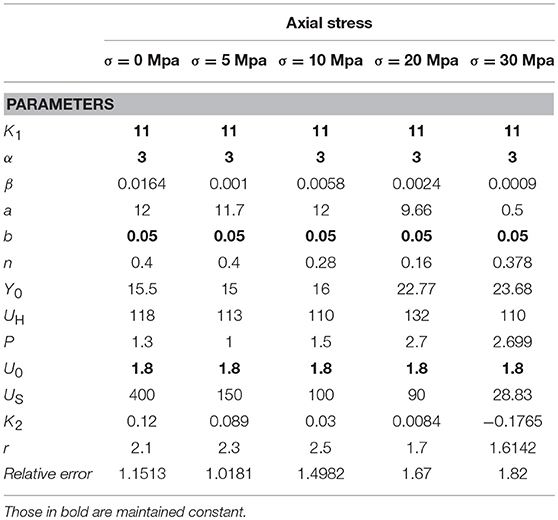
Table 4. Genetic Algorithm method: identified parameters.

FIGURE 5

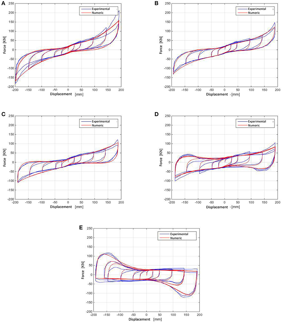
Figure 5. Genetic Algorithm method: cyclic shear test of the tested isolator (50, 100,200, 300, and 400% deformations for compression stresses of 0 MPa (A), 5 MPa (B), 10 MPa (C), 20 MPa (D), 30 MPa (E). Comparison between model (parameters in Table 4) and experimental and experimental results.

Comments on the Adopted Automatic Optimization Procedures

The Pattern Search algorithm has the benefit of requiring few optimization steps and consequently shows a faster convergence. However, it is more affected by local minima (false optimal solutions could be reached) and a starting point close to the optimal one is needed. For overcoming this aspect, the results of the human-driven procedure can help in selecting the starting point for the automatic optimization with the Pattern Search algorithm. The Genetic Algorithm method on the contrary is slower in the convergence and local minima can be overcome by exploring new extents of the domain through the genetic mutation property.

The results, as depicted by Figures 4, 5, show a satisfactory match between the numerical and experimental cycles, in particular at the lowest compression stresses (0, 5, 10 MPa). Quantitative comparison is needed for determining the optima super-set as discussed in the following.

Super-Set of Optimal Parameters

Table 5 summarizes the super-set of model parameters. This set is formed by selecting, for each value of the axial force among all the minimization procedure adopted, the parameters that minimize the error in L₂ norm of the difference between the model reaction force and the experimental one (see Equation 9). The parameters of the superset come from the Genetic Algorithm procedure, apart for the case of 10 MPa compression stress. For this case they originate from the Pattern Search procedure.

TABLE 5

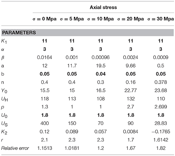
Table 5. Super-set of optimal parameters.

Figure 6 depicts the fitting laws for each parameter. Parameter β (Figure 6A) shows a variable decreasing function at increasing compression stresses. Y₀ increases linearly (Figure 6B) at the increase of the compression stresses both for compensating the shear stiffness reduction and for attaining the same plastic strains experienced at lower axial stresses. U_H shows a linear variation (Figure 6C) not far from being constant. The p variable shows an almost linear tendency (Figure 6D): it increases as the hysteresis cycles increase at higher compressive forces. Focusing now on the hardening stiffness K₂ it shows a parabolic decrease (Figure 6E), consistently with the experienced stiffness degradation due to increasing compression on the device. Amplification of hysteretic cycles at increased compression stresses is related to increment of the hardening shape related parameter r at higher compressive stresses (Figure 6F). The reduction of the U_s parameter at higher axial compression forces on the device is necessary for matching the unloading branches of the elastic-plastic component (Figure 6G). The parabolic variation of a and n parameters in Figures 6H,I allows a satisfactory transition between non-linear-elastic and elastic-plastic phases, with a reasonable reproduction of the experimental results.

FIGURE 6

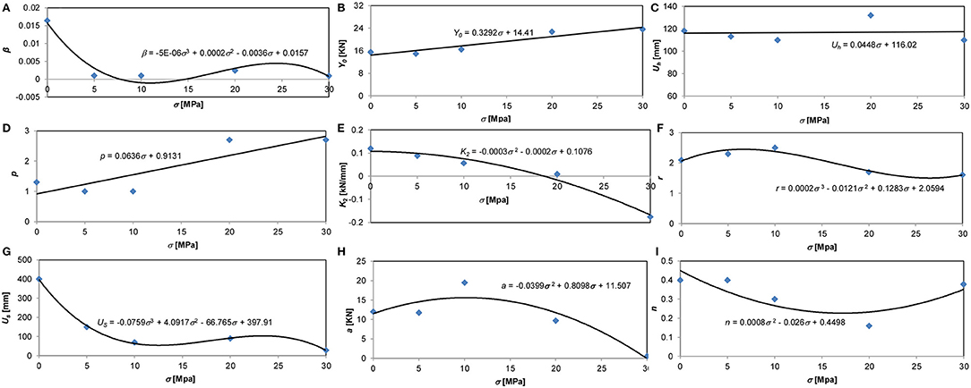
Figure 6. Fitting laws for model parameters in the Superset (A–I).

Application

In order to highlight the extent of how the horizontal response of elastomeric devices is affected by a multi-component loading, responses with and without variable axial forces are compared in this section. The time-histories of the loading components come from the response of two isolation devices located at different positions in the numerical model of a base isolated nuclear power plant (NPP—Figure 7). This was presented in Perotti et al. (2013) and studied in MATLAB (2013) and Domaneschi et al. (2012).

FIGURE 7

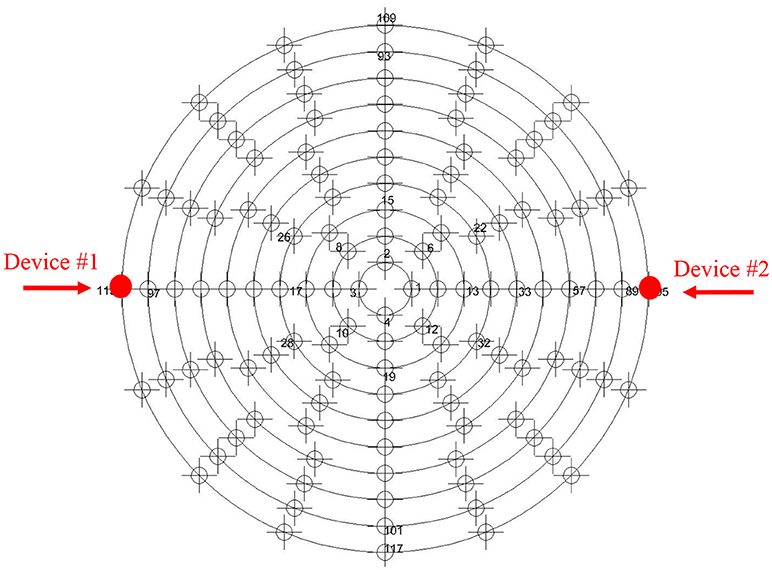
Figure 7. Plan view of the isolation system of the nuclear building in Perotti et al. (2013). Position of the devices where the time histories are collected.

FIGURE 8

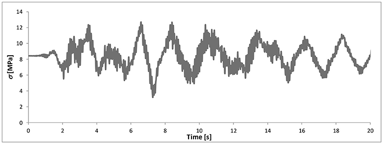
Figure 8. Time history of the axial force (in terms of stress) of device #1, used for computing the device response to variable axial force depicted in Figure 10.

FIGURE 9

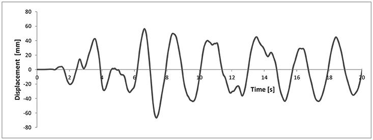
Figure 9. Time history of the relative displacement of device #1, used for computing the device response to variable axial force depicted in Figure 10.

Since the dimensions of the NPP isolation device (outside diameter D = 1,000 mm, diameter of the steel shims d = 960 mm, 10 layers of elastomeric material each 10 mm in thickness) are different from those of the device used in the Abe et al. model identification procedure (section Identification of the Model Parameters), the time histories of the loading components are scaled. Therefore, in order to impose the same value of axial stress and the same value of shear distortion in the rubber layers of both devices, the axial force of the NPP device is scaled by the ratio of the areas of the isolators, while the horizontal displacements by the ratio of the total height of the rubber layers of the devices. The variable axial load must be transformed into axial stress since all the fitting laws of the model parameters of Abe et al. are expressed in terms of axial stress values calculated in MPa.

In computing the device response through the Abe et al. model both constant and variable axial loading conditions for the device have been implemented. In the first option of constant axial loading conditions, the following values are considered: the maximum compression, the half of the maximum compression and the mean compression (static loading conditions). Following the second option, the model formulation includes the parameters dependency on axial loading in such that at any step of a time history analysis the parameters are updated.

Both Figures 10, 13 show how, as the axial force increases, the area of the hysteretic cycles increases as well. It means that the axial force variation can modify the device response and, therefore, the design isolation period and maximum lateral displacement of the isolated structure.

FIGURE 10

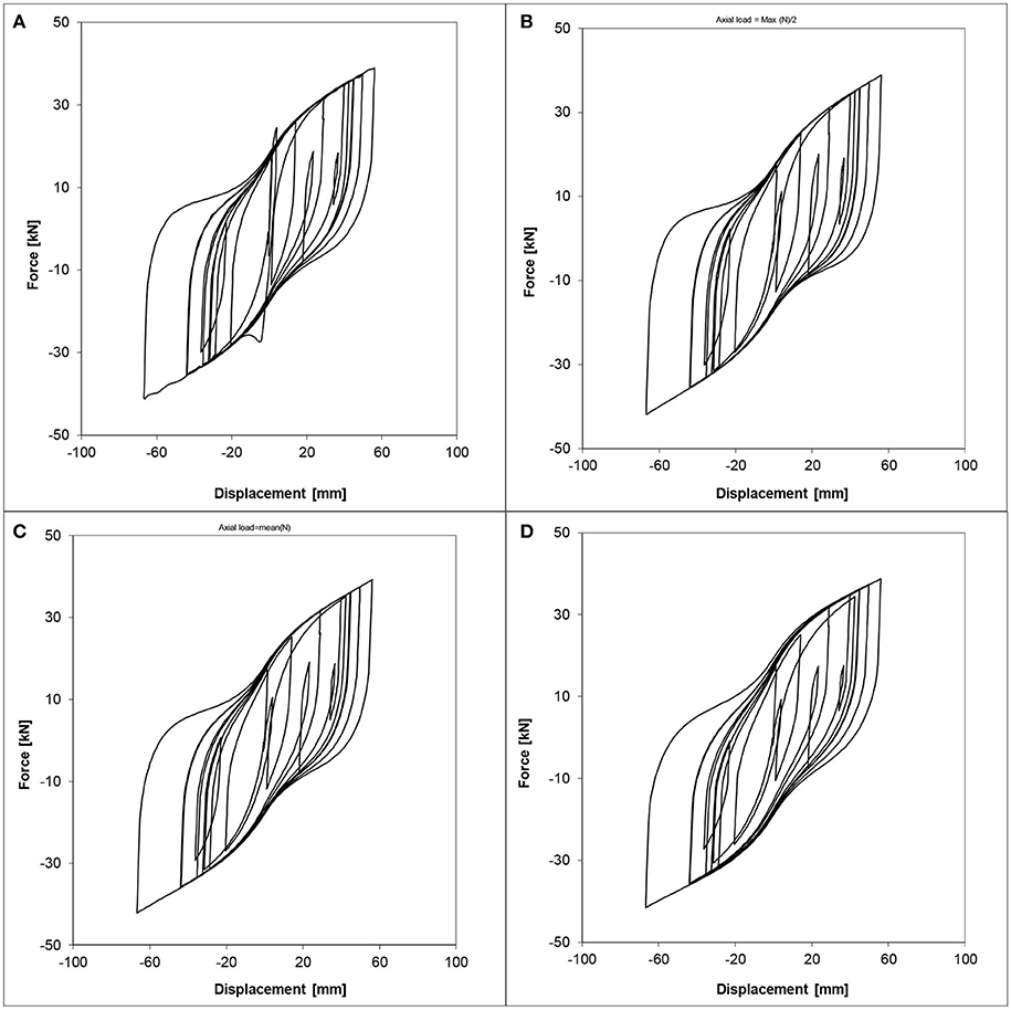
Figure 10. Lead–rubber bearing shear force–displacement hysteresis loops for device #1 with: (A) varying vertical load, (B) 6.3 MPa constant vertical stress (half of the maximum value), (C) 8.4 MPa constant vertical stress (mean value), (D) 12.6 MPa constant vertical stress (maximum value).

FIGURE 11

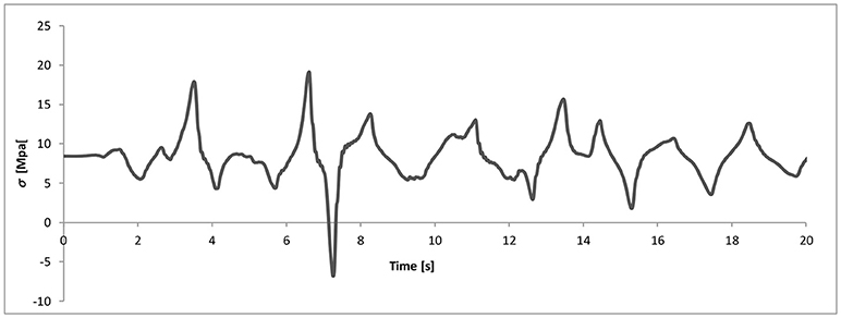
Figure 11. Time history of the axial force (in terms of stress) of device #2, used for computing the device response to variable axial force depicted in Figure 13.

FIGURE 12

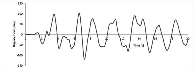
Figure 12. Time history of the relative displacement of device #2, used for computing the device response to variable axial force depicted in Figure 13.

FIGURE 13

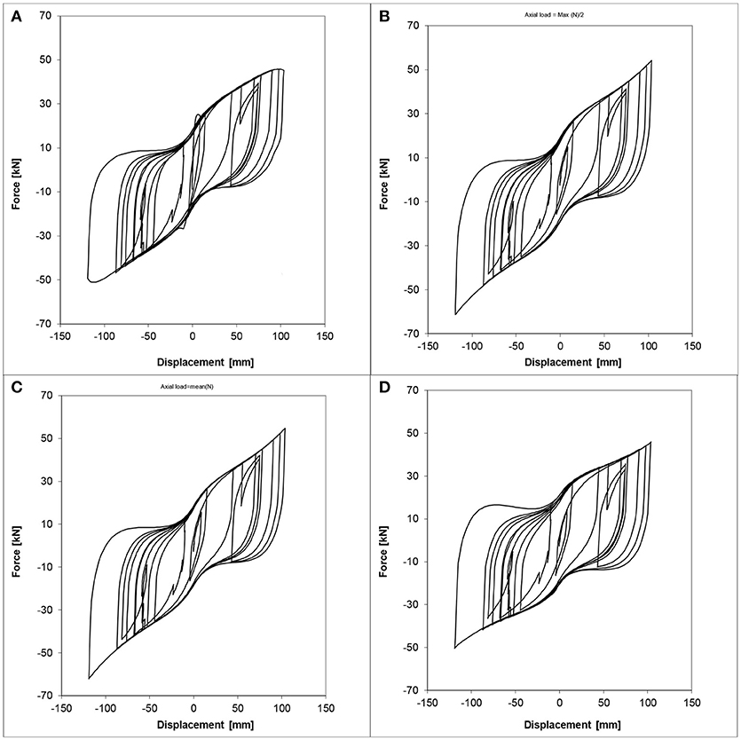
Figure 13. Lead–rubber bearing shear force–displacement hysteresis loops for device #2 with: (A) varying vertical load, (B) 9.5 MPa constant vertical stress (half of the maximum value), (C) 8 MPa constant vertical stress (mean value), (D) 19 MPa constant vertical stress (maximum value).

It can be also noted how the actual response of the device (Figures 10A, 13A) is better approximated by using the parameters derived for the maximum value of the axial force (Figures 10D, 13D), rather the lower ones (Figures 10B,C,13B,C).

Tables 6 reports the result in terms of dissipated energy over the whole loading history. No definite trend emerges, and the set of parameters coming from the lowest axial load values provide results as good (or as bad) as the other sets at the expense, however, of not reproducing correctly the lateral stiffness of the device for the highest hysteresis cycles.

TABLE 6

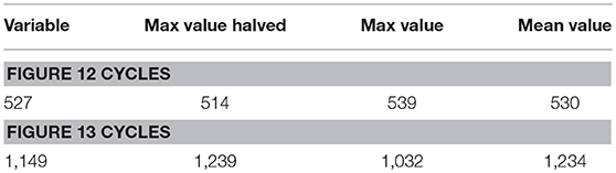
Table 6. Values of dissipated energy [J].

Conclusion

A model for simulating rubber bearings force-displacement characteristics accounting the coupled effect of variable axial loading on the horizontal response is proposed in this work. The proposed model builds upon a consolidated approach from literature, that has been demonstrated effective in reproducing the rubber bearing horizontal behavior under constant axial load. In the proposed approach, the parameters dependency on axial loading is embedded in the model formulation such that at any step of a time history analysis the parameters are updated.

The methodology adopts to available laboratory cycling tests at variable axial load, as the target for illustrating the capabilities of the new numerical procedure, and the optimization processes needed to define the model parameters. Both automatic and user-driven procedures have been used for the parameters identification.

Preliminary analyses carried out by using the proposed numerical model highlight the effects that the axial load can have on the device horizontal response. For the larger values of the axial load herein considered, this can be substantial. Subsequently, the proposed model is tested through numerical simulations on a nuclear building. The proposed model has been demonstrated effective in reproducing the coupled vertical horizontal response of the isolation system.

The proposed formulation overcomes the limits of the original model in this respect, and consistently preserves the original compactness and satisfactory representation of the experimental response for both cyclic and seismic loading at small and large value of relative displacement between the device ends.

This work is limited to the biaxial formulation (vertical-horizontal) and the general tri-axial formulation is out of the scope of this study. However, consistently with the original model, the generalization to the tri-axial version can be obtained.

Author Contributions

MD and LM worked on problems of base isolation and earthquake engineering from long time and the present development represents the most recent progress of their joined research activities. CC supported the numerical analyses as undergraduated student under the supervision of MD and LM.

Conflict of Interest Statement

The authors declare that the research was conducted in the absence of any commercial or financial relationships that could be construed as a potential conflict of interest.

References

Abe, M., Yoshida, J., and Fujino, Y. (2004a). Multiaxial behaviors of laminated rubber bearings and their modeling. I: experimental study. J. Struct. Eng. ASCE 130, 1119–1132. doi: 10.1061/(ASCE)0733-9445(2004)130:8(1119)

CrossRef Full Text | Google Scholar

Abe, M., Yoshida, J., and Fujino, Y. (2004b). Multiaxial behaviors of laminated rubber bearings and their modeling. II: modeling. J. Struct. Eng. ASCE 130, 1133–1144. doi: 10.1061/(ASCE)0733-9445(2004)130:8(1133)

CrossRef Full Text | Google Scholar

Basu, B., Bursi, O., Casciati, F., Casciati, S., Del Grosso, A., Domaneschi, M., et al. (2014). An EACS joint perspective. Recent studies in civil structural control across Europe. Struct. Control Health Monitor. 21, 1414–1436. doi: 10.1002/stc.1652

CrossRef Full Text | Google Scholar

Bhandari, M., Bharti, S. D., Shrimali, M. K., and Datta, T. K. (2017). The numerical study of base-isolated buildings under near-field and far-field earthquakes. J. Earthquake Eng. 22, 989–1007. doi: 10.1080/13632469.2016.1269698

CrossRef Full Text | Google Scholar

Dolan, E. D., Lewis, R. M., and Torczon, V. J. (2018). On the local convergence of pattern search. SIAM J. Optimizat. 14, 567–583. doi: 10.1137/S1052623400374495

CrossRef Full Text | Google Scholar

Domaneschi, M., Martinelli, L., and Perotti, P. (2012). “The effect of rocking excitation on the dynamic behavior of a Nuclear Power Plant reactor building with base isolation,” in Proceedings of the 15th World Conference on Earthquake Engineering, Lisbon. Available online at: http://www.iitk.ac.in/nicee/wcee/article/WCEE2012_2154.pdf

Google Scholar

Domaneschi, M., Martinelli, L., Perotti, P., and Tomasin, M. (2015). Assessing the performance of a high damping rubber bearing in beyond-design conditions. Proceedings of the Tenth International Workshop on Structural Health Monitoring, Stanford, CA.

Google Scholar

Han, X., and Warn, G. P. (2015). Mechanistic model for simulating critical behavior in elastomeric bearings. J. Struct. Eng. ASCE 141:04014140. doi: 10.1061/(ASCE)ST.1943-541X.0001084

CrossRef Full Text | Google Scholar

Kelly, J. M. (1997). Earthquake-Resistant Design with Rubber, 2nd Edn. London: Springer-Verlag.

Google Scholar

Kikuchi, M., and Aiken, I. D. (1997). An analytical hysteresis model for elastomeric seismic isolation bearings. Earthquake Eng. Struct. Dynam. 26, 215–231. doi: 10.1002/(SICI)1096-9845(199702)26:2&lt;215::AID-EQE640&gt;3.0.CO;2-9

CrossRef Full Text | Google Scholar

Kikuchi, M., Nakamura, T., and Aiken, I. D. (2010). Three-dimensional analysis for square seismic isolation bearings under large shear deformations and high axial loads. Earthquake Eng. Struct. Dynam. 39, 1513–1531. doi: 10.1002/eqe.1042

CrossRef Full Text | Google Scholar

Kumar, M., Whittaker, A. S., and Constantinou, M. C. (2014). An advanced numerical model of elastomeric seismic isolation bearings. Earthquake Eng. Struct. Dynam. 43, 1955–1974 doi: 10.1002/eqe.2431

CrossRef Full Text | Google Scholar

MATLAB (2013). Release R2013a User Manual, MATLAB. Natick, MA: Massachusetts.

Miller, B., and Goldberg, D. (1995). Genetic algorithms, tournament selection, and the effects of noise. Complex Syst. 9, 193–212.

Google Scholar

Perotti, F., Domaneschi, M., and De Grandis, S. (2013). The numerical computation of seismic fragility of base-isolated NPP buildings. Nuclear Eng. 262, 189–200. doi: 10.1016/j.nucengdes.2013.04.029

CrossRef Full Text | Google Scholar

Ryan, K. L., Kelly, J. M., and Chopra, A. (2005). Nonlinear model for lead-rubber bearings including axial-load effects. J. Struct. Eng. ASCE 131, 1270–1278. doi: 10.1061/(ASCE)0733-9399(2005)131:12(1270)

CrossRef Full Text | Google Scholar

Vemuru, V. S. M., Nagarajaiah, S., and Mosqueda, G. (2003). Coupled horizontal–vertical stability of bearings under dynamic loading. Earthquake Eng. Struct. Dynam. 45, 913–934 doi: 10.1002/eqe.2691

CrossRef Full Text | Google Scholar

Yamamoto, S., Kikuchi, M., Ueda, M., and Aiken, I. D. (2009). A mechanical model for elastomeric seismic isolation bearings including the influence of axial load. Earthquake Eng. Struct. Dynam. 38, 157–180. doi: 10.1002/eqe.847

CrossRef Full Text | Google Scholar