Parameter Estimation of Autoregressive-Exogenous and Autoregressive Models Subject to Missing Data Using Expectation Maximization

Introduction

A fundamental task in a variety of fields is extracting useful statistical information from time series data. Working with complete datasets, there are different tools toward this end. However, in certain applications, the datasets are faced with the possibility of missing measurements. For example, these may result from network communication disruptions, malfunctioning sensing equipment, improper sampling protocol, or observation patterns inherent to the data collection schemes (Little and Rubin, 2002; Matarazzo and Pakzad, 2015).

Missing data may present several problems for statistical analyses conducted and decisions made as a result of those analyses. If missing value indicators are not present in a data analysis package, inferences about the system being sampled can be biased. Similar biased inferences may result if missing observations are ignored, particularly if an observation's missingness is a function of its value, for example when observations are uncharacteristically orders-of-magnitude atypical. Additionally, simply from a cost perspective, it is not desirable to spend time and resources collecting data that eventually goes unused.

It follows then that researchers should seek out data analysis methods that maximize the utility of their entire dataset, incorporating the fact that it may contain missing observations. In Little and Rubin (2002), missing data methods are grouped into four non-mutually exclusive categories. Procedures based on completely recorded units encompass strategies like those described above, which essentially ignore incomplete observations, and may result in serious biases, particularly with large quantities of missing data. Weighting procedures modify response design weights in an attempt to account for missing data as if it were part of the sample design. Imputation-based procedures fill in missing values, and then analyze the complete estimated sample with standard methods. Finally, model-based procedures define a model for the observed data on which to base statistical inferences. The work presented in this paper represents a particular model-based procedure where regression models are fit to observed datasets.

Regressions represent a broad class of models that may be fit to time series data, and in our case lead to statistical inferences about that data. Model-based missing data procedures are used in conjunction with these fits to estimate their parameters. These parameters may then further be used to predict future system responses, or as indicators of changes to the system over time. In either case, accurate parameter estimation is paramount for correct system behavior prediction and assurance that any changes in regression parameters are due to system changes, as opposed to biased estimation.

This paper concerns parameter estimation of two particular types of regression models. The autoregressive-exogenous, or ARX(n, m) model assumes that current system output is a function of the previous n system outputs and previous m system inputs. The autoregressive, or AR(n) model assumes that current system output is only a function of the n previous system outputs. Both models considered in this study are used to generate simulated datasets; such datasets with missing samples are then used in this study. The algorithm presented in Section Parameter Estimation Algorithm is used for regression parameter estimation and dataset reconstruction, and the estimated parameters and measurements are compared with references. In all cases, we do not explore loss of the entire dataset, as the algorithm requires at least a portion to be run. This algorithm joins a relatively minor list of those dedicated to regression models, and more specifically ARX models, subject to missing observations. Important modifications to the state vector considered in the presented state-space model are presented.

In this paper, a specific real-world example relating to structural health monitoring (SHM) is presented, an application which has not been previously explored with the modified algorithm outside of preliminary work by the authors in Horner and Pakzad (2016a,b).

Structural vibration data has popularly been used in the field for system identification (Juang and Pappa, 1985; James III et al., 1993; Andersen, 1997; Huang, 2001; Pakzad et al., 2011; Dorvash and Pakzad, 2012; Chang and Pakzad, 2013, 2014; Dorvash et al., 2013; Cara et al., 2014; Matarazzo and Pakzad, 2016c; Nagarajaiah and Chen, 2016), finite element model updating (Shahidi and Pakzad, 2014a,b; Yousefianmoghadam et al., 2016; Nozari et al., 2017; Song et al., 2017), and damage-sensitive feature extraction (Sohn et al., 2001; Gul and Catbas, 2009; Kullaa, 2009; Dorvash et al., 2015; Shahidi et al., 2015), with the ultimate goal of inferring information about the current condition of the monitored structure. Regarding regression models, He and De Roeck (1997) shows their utility for describing structural vibration responses, and Shahidi et al. (2015) and Yao and Pakzad (2012) provide structural damage-sensitive features created using the parameters of regression models.

In this paper, acceleration time series data is collected from a two-bay structural steel frame. Parameters are estimated for ARX models using only portions of these datasets. This work extends and generalizes that introduced in Horner and Pakzad (2016b), which included a specific missing data pattern and alternative parameter estimation algorithm, and Horner and Pakzad (2016a), which used the same algorithm, but was specific to randomly missing data.

This paper is organized as follows. Section Model and Method Review provides a literature review on the relevant regression models and estimation of their parameters in the presence of missing data, as well as general likelihood model-based missing data procedures. Section Parameter Estimation Algorithm presents the proposed algorithm and highlights its differences from previous work. Section Experimental setup and simulation outlines the data collection and simulation schemes, with Section Results and Discussion presenting the validation results of regression model estimation with incomplete experimental datasets. Finally, Section Conclusions outlines the current conclusions of this work and suggestions on future research directions.

Model and Method Review

Regression Parameter Estimation

The ARX(n, m) model is defined:

$\begin{array}{l}y(k)=a_{1}y(k-1)+a_{2}y(k-2)+\cdots +a_{n}y(k-n)\\ +b_{1}u(k-1)+b_{2}u(k-2)+\cdots +b_{m}u(k-m)+v(k)& (1)\end{array}$

where y is the model output; u is the model input; a_i is the ith autoregressive (AR) parameter; b_i is the ith exogenous (X) parameter; and v is the noise. In solving the problem of parameter identification, a model is also assumed for the ARX input u. In this paper, an AR(p) model is used:

$\begin{array}{ll}u(k)=c_{1}u(k-1)+c_{2}u(k-2)+\cdots +c_{p}u(k-p)+w(k)& (2)\end{array}$

where c_i is the ith assumed input AR parameter and w the noise. In this paper, both noise terms are assumed as Gaussian white noise, with E[v²(k)] = λ₁ and E[w²(k)] = λ₂, uncorrelated with one another.

Existing literature concerning parameter identification of ARX models includes Isaksson (1993), which presents an algorithm similar to that in this paper, using both the expectation maximization (EM) algorithm and Kalman filter for parameter identification with simulated datasets. Wallin and Isaksson (2000) present an iterative algorithm using least squares and a bias correction for parameter identification that does not require an assumed input model. Wallin and Isaksson (2002) investigate periodic missing data patterns and multiple optima that may result when input data is missing. Wallin and Hansson (2014) proposes an algorithm separate from EM for a wide class of models, including ARX. Ding et al. (2011) use gradient-based parameter identification methods with structural vibration data. Finally, Naranjo (2007) discusses general state space models with exogenous variables and missing data.

The algorithm proposed in this paper can also identify the parameters of AR models alone, of the form in Equation (2). The literature is more extensive on parameter estimation of these models. Papers with a similar approach that utilize maximum likelihood (ML) and EM-based approaches include McGiffin and Murthy (1980, 1981), which provide simulation results for a variety of parameter estimation methods. Kolenikov (2003) and Little and Rubin (2002) investigate parameter estimation for AR(1) models. Sargan and Drettakis (1974) present a ML approach that treats missing observations as additional parameters with respect to which the likelihood is maximized. Broersen and Box (2006) perform ML parameter estimation on AR, MA, and ARMA models. Zgheib et al. (2006) present a pseudo-linear recursive least squares algorithm in conjunction with the Kalman filter for reconstruction and AR parameter identification. Finally, Shumway and Stoffer (2000) present an overview of state space models and modifications with missing data. There are several important distinctions between the proposed algorithm and those presented in previous works; these will be presented as they arise in Section Parameter Estimation Algorithm. Additionally, this paper includes both real and simulated datasets for ARX models.

In each case presented in this paper's results, the model order must be selected prior to parameter estimation and dataset reconstruction. While the paper does explore the effects of selecting a different model order than that used to generate the dataset (see Section Improper Model Order Selection—Simulated), evaluation of strategies for selecting the correct or most-likely model order are beyond the scope of this work. To this end, there are several studies, including Grossmann et al. (2009) and Matarazzo and Pakzad (2016b), which discuss that the model order decreases significantly with an increase in missing data. Additionally, Sadeghi Eshkevari and Pakzad (2019) emphasize that randomness in missing data results in lower model order selection.

Maximum Likelihood, Expectation Maximization, and Kalman Filter

A review of maximum likelihood estimation (MLE) and the expectation maximization (EM) algorithm is provided in Little and Rubin (2002). The idea behind the former is to find the values of some statistical parameters that maximize a likelihood function associated with the sampled data. This likelihood function is proportional to the probability density function of the data (often the logarithm of the probability density function, or “log-likelihood”). EM is an iterative strategy for MLE in incomplete data problems. It formalizes the procedure to handle missingness of estimating data values, estimating parameters, re-estimating data values assuming the parameters are correct, and iterating until convergence.

The idea of MLE is used extensively in the literature. Specifically for regression models, MLE without EM is discussed in Wallin and Hansson (2014) for several regression model classes, McGiffin and Murthy (1980, 1981) and Sargan and Drettakis (1974) for AR models, Dunsmuir and Robinson (1981) and Jones (1980) for autoregressive-moving-average (ARMA) models, and ARX models in Wallin and Isaksson (2002).

The EM algorithm was first formally defined in Dempster et al. (1977), which outlines several important characteristics, namely, that it is applicable to a wide array of topics, that successive iterations always increase the likelihood, and that convergence implies a stationary point of the likelihood. Shumway and Stoffer (1982) and Digalakis et al. (1993) describe the algorithm's utility with stochastic state-space models in conjunction with the Kalman filter. Mader et al. (2014) introduce a numerically efficient implementation of EM. The algorithm similar to that of this paper presented in Isaksson (1993) utilizes EM for ARX parameter identification. In the context of structural vibrations with missing data, EM is used in mobile sensing for system identification in Matarazzo and Pakzad (2014, 2015, 2016a,b).

Recall that the idea behind EM involves estimating missing values, or more generally, sufficient statistics of the missing observations so as to determine the model parameters (i.e., the “E” step). With the exception of Dempster et al. (1977), the EM papers above all utilize the Kalman filter (Kalman, 1960) to this end, as do Shi and Fang (2010) for randomly missing data. This recursive algorithm produces state variable estimates by prediction at each time step, then updating the estimates as a new measurement is taken. The estimates are then more “precise” than the measurements, which are naturally corrupted with noise. ARMA model parameters are identified with the Kalman filter and EM by Harvey and Phillips (1979), Jones (1980), Harvey and Pierse (1984). AR models are considered using a Kalman filter formulation in McGiffin and Murthy (1981), Zgheib et al. (2006), and Wallin and Isaksson (2002) identify multiple optima in ARX models with Kalman parameter identification. In Section Parameter Estimation Algorithm, the algorithm introduced in this paper is presented, incorporating the Kalman filter in the expectation step of the EM algorithm for MLE of ARX and AR parameters.

Parameter Estimation Algorithm

Underlying State-Space Model

The algorithm proposed in this paper can be used for parameter estimation of either ARX or AR models. We introduce the algorithm here for general ARX(n, m) models and provide guidance for its adaption to AR(n) models. Two important differences from the formulation in Isaksson (1993) are presented here. In Section Experimental Setup and Simulation, the real data considered for testing the proposed algorithm constitutes structural vibrations. In this context, y and u in Equations 1, 2 represent structural responses at two distinct locations. Note here that u does not constitute an “input” to the system; nevertheless, we will use the term “input” when referring to the u data in this paper. Using alternative terminology, such an ARX model represents a transmissibility function from different system responses.

For the remainder of this paper, m = n is assumed for the ARX model orders (this is not required, but it eases notation clarity). Define z(k), A_i, and e(k) for ARX models, as:

$\begin{array}{l}z(k)=\left[\begin{array}{c}y(k)\\ u(k)\end{array}\right]A_i=\left[\begin{array}{cc}{a}_i& b_i\\ 0& {\text{c}}_i\end{array}\right]e(k)=\left[\begin{array}{c}v(k)\\ w(k)\end{array}\right]\\ \text{E}\left[e(k)e^T(k)\right]=\Lambda =\left[\begin{array}{cc}{\lambda }_1& 0\\ 0& {\lambda }_2\end{array}\right]\end{array}$

assuming the two noise variance terms are uncorrelated. For AR models:

$\begin{array}{l}z(k)=y(k)A_i=a_i\text{E}\left[e(k)e^T(k)\right]=\Lambda ={\lambda }_1\end{array}$

Equations (1, 2) may be rewritten as:

$\begin{array}{l}z(k)=A_{1}z(k-1)+A_{2}z(k-2)+\cdots \\ +A_{l}z(k-l)+e(k)& (3)\end{array}$

where l is the largest of n (or m) and p.

The Kalman filter (Section Kalman Filter) is employed for reconstruction of missing observations; models for use with this filter may be in state-space form. The choice of a state vector for this model is not trivial as is shown in the EM algorithm parameter estimates of Section EM Algorithm. The state vector x(k) is given below:

$\begin{array}{l}x(k)={\left[\begin{array}{cccc}{z}^T(k)& z^T(k-1)& \cdots & z^T(k-n)\end{array}\right]}^T\end{array}$

and the state-space equations may then be written as:

$\begin{array}{ll}x(k)=Fx(k-1)+e(k)& (4)\end{array}$

$\begin{array}{ll}z(k)=Hx(k)& (5)\end{array}$

with the following state matrix F and output matrix H (note that all matrix entries shown below are 2 x 2 in size for ARX models):

$\begin{array}{l}\hfill F=\left[\begin{array}{cccccc}{A}_1& A_2& \cdots & A_{n-1}& A_n& 0\\ I& 0& \cdots & 0& 0& 0\\ 0& I& \cdots & 0& 0& 0\\ ⋮& ⋮& \ddots & ⋮& ⋮& ⋮\\ 0& 0& \cdots & I& 0& 0\\ 0& 0& \cdots & 0& I& 0\end{array}\right]\\ H=\left[\begin{array}{cccccc}I& 0& \cdots & 0& 0& 0\end{array}\right]\end{array}$

In Isaksson (1993), the H matrix is [A₁ A₂ … A_n−1 A_n] where it is composed of unknown model parameters. The choice of state vector here, which differs by a lag of one time step, simplifies the H matrix by fixing it to the above. This removes the uncertainty in H and reduces the complexity of the system identification computations for the case where the kth measurement is included in the kth state vector.

The last pieces required to use the Kalman filter are the covariance matrices of the process and measurement noise. Since the kth measurement is included in the kth state vector, the measurement equation noise term is not included [see Equation (5)], and its covariance matrix R = [0]. Due to the identity elements along a lower diagonal of F, only the first (AR) or first two (ARX) terms along the diagonal of the process covariance matrix Q are nonzero, and are equal to Λ.

Kalman Filter

For complete datasets, the matrices of Equation (5) and the noise covariances are fed to the Kalman filter directly with the data to find filtered state estimates, and the parameter estimation algorithm continues with EM (see Section EM Algorithm). The Kalman filter “predictive” equations are presented below:

$\begin{array}{ll}{\widehat{x}}^{-}(k)=F\widehat{x}(k-1)& (6)\end{array}$

$\begin{array}{ll}{P}^{-}(k)=FP(k-1)F^T+Q& (7)\end{array}$

where ∧ denotes an estimate; ⁻ denotes that the value is a priori; x and P quantities without a ⁻ are a posteriori; and P(k) is the error covariance at time k. The Kalman filter “corrective” equations update the a priori estimates and are given in Equations (8–10):

$\begin{array}{ll}K(k)=P^{-}(k)H^T{\left(H{P}^{-}(k)H^T+R\right)}^{-1}& (8)\end{array}$

$\begin{array}{ll}\widehat{x}(k)={\widehat{x}}^{-}(k)+K(k)\left(z(k)-H{\widehat{x}}^{-}(k)\right)& (9)\end{array}$

$\begin{array}{ll}P(k)=(I-K(k)H)P^{-}(k)& (10)\end{array}$

where K(k) is the Kalman gain at time k. In addition to the state and output matrices, the Kalman filter requires initial state and error covariance estimates, selection of which is discussed in Section Results and Discussion.

To produce state estimates at time steps with missing measurements, the filter must also be made aware not to “trust” measurements indicating a time step with missing observations, be they zero values, NaN indicators, or values orders of magnitude-atypical. The output matrix H and measurement noise covariance R are thus indexed to each time step k. Only values in these matrices pertaining to non-missing observations are sent to the filter. For example, in the case of a missing input at time step k, a matrix D(k) is defined to indicate the output observation as the only trusted measurement. In the case of Equation (5) for an ARX model, the measurement vector z(k) would then be length two, and D(k) then would be the first row of a 2 × 2 identity matrix. For any D(k), H(k), and R(k) are then defined:

$\begin{array}{ll}H(k)=D(k)H& (11)\end{array}$

$\begin{array}{ll}R(k)=D(k)R{D}^T(k)& (12)\end{array}$

Recall, however, that the covariance matrix R = [0], thus always evaluating Equation (12) to [0] as well.

EM Algorithm

The EM algorithm is used to produce MLEs of the unknown parameters for the system, including the error variance terms λ₁ and λ₂, and all regression parameters. The basis for this algorithm lies in definition of the log-likelihood equation of the reconstructed dataset; formerly-missing observations are contained in the states estimated using the Kalman filter. First, the ARX model presented in Equations (1–3) is given new notation:

$\begin{array}{ll}y(k)={\varphi }_1^T(k){\theta }_1+v(k)& (13)\end{array}$

$\begin{array}{ll}u(k)={\varphi }_2^T(k){\theta }_2+w(k)& (14)\end{array}$

where:

$\begin{array}{l}{\varphi }_1(k)=\left[\begin{array}{c}y(k-1)\\ u(k-1)\\ ⋮\\ y(k-n)\\ u(k-n)\end{array}\right]{\theta }_1=\left[\begin{array}{c}{a}_1\\ b_1\\ ⋮\\ a_n\\ b_n\end{array}\right]\\ {\varphi }_2(k)=\left[\begin{array}{c}u(k-1)\\ ⋮\\ u(k-p)\end{array}\right]{\theta }_2=\left[\begin{array}{c}{c}_1\\ ⋮\\ c_p\end{array}\right]\end{array}$

The response is uncorrelated to the excitation for positive time lags. In other words, the response at one time is uncorrelated to the excitation at any time after that. Therefore, model output and input can be considered as independent Gaussian processes. Using the notation above, the joint density of all N observations, denoted f, may be written as:

$\begin{array}{ll}f={\displaystyle \prod _{k=1}^N}\left(\left\{\frac{1}{\sqrt{2\pi {\lambda }_1}}\text{exp }\left[\frac{-{\left(y(k)-{\varphi }_1^T(k){\theta }_1\right)}^2}{2{\lambda }_1}\right]\right\}\left\{\frac{1}{\sqrt{2\pi {\lambda }_2}}\text{exp }\left[\frac{-{\left(u(k)-{\varphi }_2^T(k){\theta }_2\right)}^2}{2{\lambda }_2}\right]\right\}\right)& (15)\end{array}$

Taking the natural logarithm of this equation yields the log-likelihood criterion:

$\begin{array}{lll}L(\theta ,\Lambda )& =& C-\frac{N}{2}\text{log}({\lambda }_1)-\frac{N}{2}\text{log}({\lambda }_2)\\ & & -\frac{1}{2{\lambda }_1}{{\displaystyle \sum }}_{k=1}^N{\left(y(k)-{\varphi }_1^T(k){\theta }_1\right)}^2\\ & & -\frac{1}{2{\lambda }_2}{\displaystyle \sum _{k=1}^N}{\left(u(k)-{\varphi }_2^T(k){\theta }_2\right)}^2& (16)\end{array}$

Equation (16) contains the constant term C which does not affect maximization. Differentiation of this equation with respect to each of the noise variances and setting the results equal to zero gives the MLEs for the noise variance terms:

$\begin{array}{lll}{\lambda }_1& =& \frac{1}{N}{\displaystyle \sum _{k=1}^N}{E}_N\left[{\left(y(k)-{\varphi }_1^T(k){\theta }_1\right)}^2\right]\\ & =& \frac{1}{N}({{\displaystyle \sum }}_{k=1}^N{E}_N\left[y^2(k)\right]-2{\displaystyle \sum _{k=1}^N}{E}_N\left[{\varphi }_1^T(k)y(k)\right]{\theta }_1\\ & & +{\displaystyle {\sum }_{k=1}^N{\theta }_1^T{E}_N\left[{\varphi }_1(k){\varphi }_1^T(k)\right]{\theta }_1)}& (17)\end{array}$

and:

$\begin{array}{lll}{\lambda }_2& =& \frac{1}{N}{\displaystyle \sum _{k=1}^N}{E}_N\left[{\left(u(k)-{\varphi }_2^T(k){\theta }_2\right)}^2\right]\\ & =& \frac{1}{N}({{\displaystyle \sum }}_{k=1}^N{E}_N\left[u^2(k)\right]-2{{\displaystyle \sum }}_{k=1}^N{E}_N\left[{\varphi }_2^T(k)u(k)\right]{\theta }_2\\ & & +{\displaystyle {\sum }_{k=1}^N{\theta }_2^T{E}_N\left[{\varphi }_2(k){\varphi }_2^T(k)\right]{\theta }_2)}& (18)\end{array}$

where E_N denotes the conditional expectation based on observations until sample N, not the entire dataset. Substituting Equations (17, 18) into Equation (16) yields a different form of the log-likelihood:

$\begin{array}{lll}L(\theta ,\Lambda )& =& C-\frac{N}{2}\text{log }\left(\frac{1}{N}{{\displaystyle \sum }}_{k=1}^N{E}_N\left[{\left(y(k)-{\varphi }_1^T(k){\theta }_1\right)}^2\right]\right)\\ & & -\frac{N}{2}\text{log }\left(\frac{1}{N}{\displaystyle \sum _{k=1}^N}{E}_N\left[{\left(u(k)-{\varphi }_2^T(k){\theta }_2\right)}^2\right]\right)& (19)\end{array}$

Maximizing this log-likelihood is equivalent to minimizing the quantities in the log terms, so these parts of the equation are differentiated with respect to the θ parameter vectors and set to zero to yield their MLEs:

$\begin{array}{lll}{\theta }_1^{(i+1)}& =& {\left({{\displaystyle \sum }}_{k=1}^N{\text{E}}_N\left[{\varphi }_1(k){\varphi }_1^T(k)\right]\right)}^{-1}\\ & & \times {{\displaystyle \sum }}_{k=1}^N{\text{E}}_N\left[{\varphi }_1(k)y(k)\right]& (20)\end{array}$

$\begin{array}{lll}{\theta }_2^{(i+1)}& =& {\left({{\displaystyle \sum }}_{k=1}^N{\text{E}}_N\left[{\varphi }_2(k){\varphi }_2^T(k)\right]\right)}^{-1}\\ & & \times {{\displaystyle \sum }}_{k=1}^N{\text{E}}_N\left[{\varphi }_2(k)u(k)\right]& (21)\end{array}$

Thus, the EM algorithm is defined, with the expectation step encompassing the dataset completion (Kalman filtering) and Equations (16–18), and the maximization step Equations (20, 21). The algorithm iterates until some convergence criterion is reached (for the purposes of examples presented later in this paper, that criterion is achieved when the change in either variance parameter becomes <1 × 10⁻¹¹ from one iteration to the next; this threshold was selected to be within the computer's machine epsilon threshold, as well as practicality from a speed perspective. A flowchart of the proposed algorithm's key steps is defined in Figure 1.

FIGURE 1

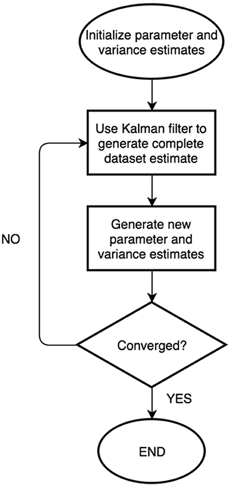
Figure 1. Proposed parameter and missing data-estimation algorithm.

One iteration of the EM algorithm requires calculation of each expectation contained in Equations (17, 18, 20, 21). As the Kalman filter provides the state estimates (which in turn correspond to the y and u values contained in the φ vectors) as well as the error covariance matrices, the appropriate quantities must simply be selected for the applicable summations. The key is to notice that the kth state vector x(k) (of length (2l + 2), for ARX) contains the kth y measurement as its first term, the kth u measurement as its second, the kth φ₁ vector as terms 3 through (2n + 2), and the kth φ₂ vector as even terms 4 through (2p + 2). The relevant covariance terms are in the corresponding rows and columns within the P(k) matrix. The required expectations are now defined in Equations (22–27), with subscripts denoting the relevant parts of the state vector and error covariance matrices:

$\begin{array}{ll}{\text{E}}_N\left[y^2(k)\right]={\widehat{x}}_1^2(k)+P_{1,1}(k)& (22)\end{array}$

$\begin{array}{ll}{\text{E}}_N\left[u^2(k)\right]={\widehat{x}}_2^2(k)+P_{2,2}(k)& (23)\end{array}$

$\begin{array}{ll}{\text{E}}_N\left[{\varphi }_1(k)y(k)\right]={\widehat{x}}_{3:(2n+2)}(k){\widehat{x}}_1(k)+P_{3:(2n+2),1}(k)& (24)\end{array}$

$\begin{array}{ll}{\text{E}}_N\left[{\varphi }_2(k)u(k)\right]={\widehat{x}}_{4:2:(2n+2)}(k){\widehat{x}}_2(k)+P_{4:2:(2n+2),2}(k)& (25)\end{array}$

$\begin{array}{lll}{\text{E}}_N\left[{\varphi }_1(k){\varphi }_1^T(k)\right]& =& {\widehat{x}}_{3:(2n+2)}(k){\widehat{x}}_{3:(2n+2)}^T(k)\\ & & +P_{3:(2n+2),3:(2n+2)}(k)& (26)\end{array}$

$\begin{array}{lll}{\text{E}}_N\left[{\varphi }_2(k){\varphi }_2^T(k)\right]& =& {\widehat{x}}_{4:2:(2n+2)}(k){\widehat{x}}_{4:2:(2n+2)}^T(k)\\ & & +P_{4:2:(2n+2),4:2:(2n+2)}(k)& (27)\end{array}$

It is in these expectation definitions that the choice of state vector becomes critical, and where the first distinction is made between this work and that of Isaksson (1993). Without including y(k) and φ₁(k), and u(k) and φ₂(k) in the same state vectors, all required error covariance terms for evaluation of Equations (22–27) would not be obtained within the Kalman filter portion of the algorithm. Isaksson (1993) appears to only include all terms in the k + 1 state vector.

For AR models, there are modifications to the EM algorithm. Vectors with subscript 2, and thereby Equations (14, 18, 21, 23, 25, and 27) are no longer needed. φ₁(k) and θ₁ are redefined as:

$\begin{array}{l}{\varphi }_1(k)=\left[\begin{array}{c}y(k-1)\\ y(k-2)\\ ⋮\\ y(k-n)\end{array}\right]{\theta }_1=\left[\begin{array}{c}{a}_1\\ a_2\\ ⋮\\ a_n\end{array}\right]\end{array}$

and Equations (15, 19, 24, 26) are rewritten as Equations (28–31), respectively, below:

$\begin{array}{ll}f={\displaystyle \prod _{k=1}^N}\left\{\frac{1}{\sqrt{2\pi {\lambda }_1}}\text{exp }\left[\frac{-{\left(y(k)-{\varphi }_1^T(k){\theta }_1\right)}^2}{2{\lambda }_1}\right]\right\}& (28)\end{array}$

$\begin{array}{ll}L(\theta ,\Lambda )=C-\frac{N}{2}\text{log }\left(\frac{1}{N}{\displaystyle \sum _{k=1}^N}{E}_N\left[{\left(y(k)-{\varphi }_1^T(k){\theta }_1\right)}^2\right]\right)& (29)\end{array}$

$\begin{array}{ll}{E}_N\left[{\varphi }_1^T(k)y(k)\right]={\widehat{x}}_{2:(n+1)}(k){\widehat{x}}_1(k)+P_{1,2:(n+1)}(k)& (30)\end{array}$

$\begin{array}{lll}{E}_N\left[{\varphi }_1(k){\varphi }_1^T(k)\right]& =& {\widehat{x}}_{2:(n+1)}(k){\widehat{x}}_{2:(n+1)}^T(k)\\ & & +P_{2:(n+1),2:(n+1)}(k)\end{array}$

The second key difference between the proposed algorithm and that presented in Isaksson (1993) is simply that it stops here; we have not employed the Rauch-Tung-Striebel (RTS) smoother in this paper, as simulations conducted with it did not show a difference in model utility. However, the formulation is kept consistent for the case where smoother operations can be applicable. Please note that the proposed filtering can be implemented in real-time, while the suggested smoothing operations need offline computations. In some applications, the advantage of real-time filtering might be more desirable than the accuracy of the results; implementation of the proposed algorithm for online EM is thus the subject of future work. The ability of this algorithm to identify the correct parameters of incomplete datasets is evaluated in the following sections.

Experimental Setup and Simulation

The proposed algorithm is tested on both experimentally-collected, and simulated datasets. When practical, the experimental datasets are used. There are a variety of variables that may affect the convergence behavior of the algorithm. We investigate the effects of varying percentage of missing data; pattern of missing data; improper model order selection; variable AR, X, and input AR model order; noise level; and model type (ARX vs. AR) on the speed of convergence and accuracy of both parameter and completed dataset estimates. In all instances, some portion of the data set was left intact to allow the algorithm to be run—at most, we considered up to 80% missingness in a packet-loss scenario. The majority of investigation results are presented in Section Results and Discussion as box plots. Each box represents the results of 200 simulations according to the prescribed conditions. In the case of randomly missing data, indices of missingness were selected with MATLAB's random number generation scheme.

Missing data indices were kept the same across sets of 200 iterations. This would ensure that the variability in a given box plot was associated only with the initial parameter guesses. These were always randomly generated, but so as to ensure a stationary model. For example, all ARX parameters were limited within (−1/max(n, m), 1/max(n, m)). Initial noise variance estimates were set at 0.01, as this seemed to obtain good results across the board in all simulations. The initial state vector was simply the first (2l + 2) measurements, and the initial Kalman error covariance matrix was the identity matrix.

The quantity typically selected for evaluation of parameter estimate accuracy is the root mean square of the normalized error (RMSNE). The RMSE (note the lack of normalization) is described in Chai and Draxler (2014); we elect to include normalization as we look at both parameter convergence, and adequacy of dataset reconstruction. Equation (32) defines the RMSNE:

$\begin{array}{ll}\text{RMSN}\text{E}=\sqrt{\frac{1}{M}{{\displaystyle \sum }}_{j=1}^M{\left(\frac{p_m-p_f}{p_f}\right)}^2}& (32)\end{array}$

where p_m is the estimated point (be it a parameter or a data point) from the missing data analysis; p_f is the corresponding full data estimate (or true value); and M is the number of values in a given estimate vector. In calculating RMSNE values when p_f is near-zero, large values may result; for this reason, we have elected not to include points in RMSNE calculations when the actual values are below a tolerance, in this case 0.001.

Structural Vibration Data

The real dataset used in this paper consists of the responses from two of the sensors in one of 39 tests outlined in Nigro and Pakzad (2014) on a two-bay, structural steel frame. The collected data represents structural acceleration responses to an impulse load. Figure 2A shows the (highlighted) frame within the laboratory, with Figure 2B presenting an elevation drawing with the sensors of concern and impulse loading location. The responses from sensor L5 were considered as the “output” or y values of the ARX model, with L4 constituting the “input” u values. These sensor designations are used so as to ease the cross-referencing of this work with that in Nigro and Pakzad (2014) and Shahidi et al. (2015). The test lasted 2 s and each wireless sensor had 500 Hz sampling rates, yielding 1,000 total measurements apiece. The amplitude-limited impulse excitation was selected due to the assumption of linear behavior for the frame. The impulse also does not impose a specific frequency onto the frame. This represents an advantageous similarity to ambient vibration (Shahidi et al. 2015), the most likely condition during which monitoring of a real structure would occur.

FIGURE 2

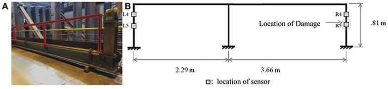
Figure 2. (A) Two-bay structural steel frame. (B) Sensor locations and frame dimensions.

Simulated Data

The simulated dataset used in this paper was selected to be similar to that obtained from the experimental setup above, but more easily controlled. We began by fitting an ARX(4, 4) with input AR(4) model to the experimental datasets [this model order was selected due to its good results in Shahidi et al. (2015)]. Then, the MLE parameters were simply used as the “true” parameters with which to generate entirely new “output” (and input, for ARX) datasets. Normally-distributed randomly-generated noise could also be added with controllable mean and variance. In all cases, the initial output and input values for the generated datasets were set to unity. With the exception of the noise variances, the same parameters were used for generation of simulated datasets at all times. These (rounded) are provided in Table 1.

TABLE 1

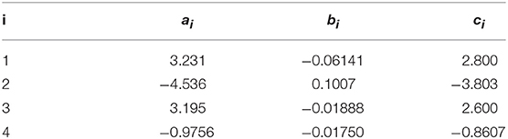
Table 1. ARX parameters for generation of simulated datasets.

Results and Discussion

Variable Missing Data Pattern—Experimental

Three missing data patterns were investigated for experimental data with ARX models. Figure 3 displays the results of variable random missing data percentages. Missing data indices were randomly generated in MATLAB. This may represent intermittent, random sensor network communication disruptions in the real world. Figure 4 displays the results of variable block missing data percentages. This represents the case of a packet-loss scenario in the real world. The location within the dataset of the block of missing data was confined to the middle of each dataset. Figure 5 displays the results of variable repetitive patterns of missing data. This represents a more predictable sensor communication disruption pattern. In each case, missing data was simulated for both output and input data.

FIGURE 3

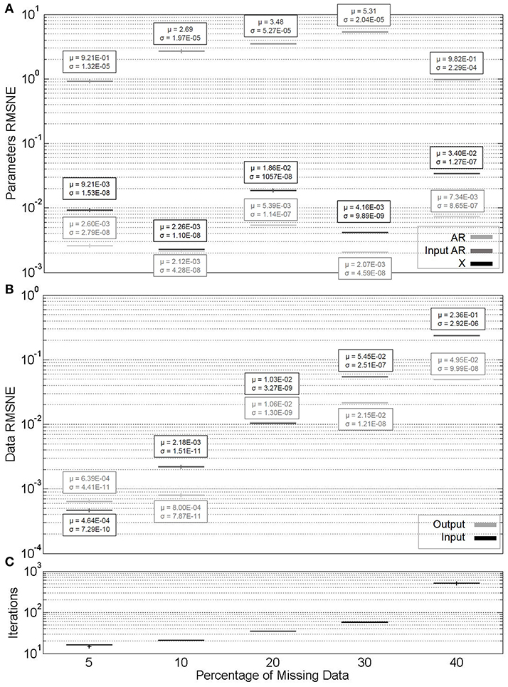
Figure 3. (A) Parameter estimate convergence for different percentages of randomly missing data. (B) Measurement estimate convergence. (C) Iterations to convergence.

FIGURE 4

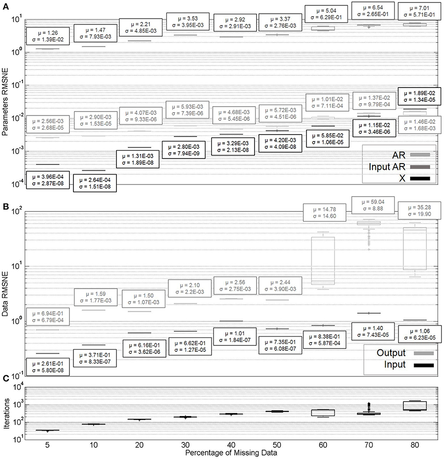
Figure 4. (A) Parameter estimate convergence for different percentages of block missing data. (B) Measurement estimate convergence. (C) Iterations to convergence.

FIGURE 5

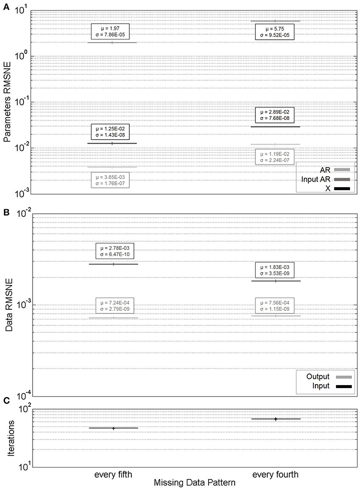
Figure 5. (A) Parameter estimate convergence for different percentages of repeating pattern missing data. (B) Measurement estimate convergence. (C) Iterations to convergence.

In each of Figures 3–5, the horizontal axes labels indicate the pattern (or percentage) of missing indices along the length of the dataset. In all cases, an ARX(4, 4)with input AR(4) model was considered. For each missing data pattern or percentage, 200 simulations were run. The (A) portions of each figure represent box plots of the parameter RMSNE values for these ten simulations, and the (B) portions the same for the data RMSNE values. In each parameter figure, the lightest box plots indicate AR parameters, the medium-hued X parameters, and the darkest input AR parameters. In each data figure, the lighter box plots indicate output data, and the darker input data. The theoretically “correct” parameters are not known for the experimental dataset; for comparison in RMSNE calculations, we use the results of EM parameter estimation on the complete dataset (without Kalman filtering).

The results of the above simulations are as expected. We are primarily concerned with parameter estimation, so the fact that there does not appear to be a great difference in accuracy of the parameter estimates across different missing data patterns is as intended for a robust parameter estimation algorithm. It is worth noting that the X parameters tend to have significantly higher RMSNE values across all missing data percentages than the AR or input AR parameters. This is likely largely in part due to the X parameters being significantly smaller in magnitude than the AR or input AR parameters.

Of some concern is the drastic increase in data reconstructive error for block missingness compared to random or patterned missingness, and particularly the variability in this error at high missingness percentages. This phenomenon occurs due to the MLE model causing the Kalman estimates to go to zero at a swifter rate than the actual system. This implies that the algorithm, in its current state, works adequately for parameter estimation with a variety of missing data patterns, but is not particularly appropriate for dataset reconstruction in the case of packet loss, or prediction. This effect additionally begins to affect the parameter estimate reliability and convergence rate as well-beyond 60 percent missingness. However, this is not the only factor at play, since there may be other regression models (or different orders) that simply fit the dataset better.

It may appear that cases of patterned missingness, as opposed to block or random, have less variability in the accuracy of the estimated parameters and reconstructed datasets, as well as number of iterations to convergence. However, if missing every fifth observation is thought of as missing 20 percent of observations (and furthermore, every fourth as 25 percent), we appear to see similar variation as at these percentages for random and block missingness. Finally, note the termination percentages for the Figures 3, 4 horizontal axes. In this section, and beyond, the criterion for these termination procedures was that the algorithm became impractically slow to converge. This suggests that packet loss scenarios, with their caveat on reconstruction, may still be handled with the algorithm for parameter estimation, and at higher percentages of missing data than random or patterned-missingness.

Improper Model Order Selection—Simulated

The purpose of this section is to evaluate the effectiveness of the algorithm for parameter identification and dataset completion when a model is generated with a different series of model orders than that used for the fit in the algorithm. In each simulation, the procedure described in Section Simulated Data was used for model generation [i.e., it was ARX(4, 4) with AR(4)], all with 20% missing data. Cases of overparameterization were explored in these simulations, and would invalidate typical RMSNE calculations for the parameters. Therefore, a different means of presenting parameter convergence is shown in Figure 6. The horizontal axis of this plot shows the number of iterations required for converged parameter estimates; thus, each vertical column of parameter estimates corresponds to the results of the same simulation. From left to right in the figure, the vertical columns represent 2nd, 6th, 3rd, 5th, and 4th order ARX model parameters. The vertical axis shows the signed logarithm of the parameter magnitude (SLPM), defined in Equation (33):

$\begin{array}{ll}\text{SLPM}=sgn(p_i)\times \text{log}\left(\left|p_i\right|\right)& (33)\end{array}$

where p_i represents a particular parameter value. The logarithm of this quantity is selected to properly display parameters of very different magnitudes on the same plot, and the sign function is selected to include both positive and negative values on the plot. In Figure 6, the large symbols at the right end of the horizontal lines represent the true parameter values of the ARX(4, 4) and input AR(4) models used for dataset generation (note then that these are NOT representative of convergence behavior in the axis-limit-number of iterations). Symbols within the figure correspond to those of the fits. Symbols occurring within the plots, but without corresponding border symbols (and indicated), were thus determined from higher-than-fourth-order models. Figure 7, alternatively, uses the same conventions as above for data value RMSNE calculations.

FIGURE 6

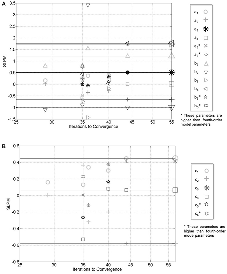
Figure 6. (A) Convergence behavior of ARX parameter estimates with varying model order fits for simulated dataset. (B) AR parameters.

FIGURE 7

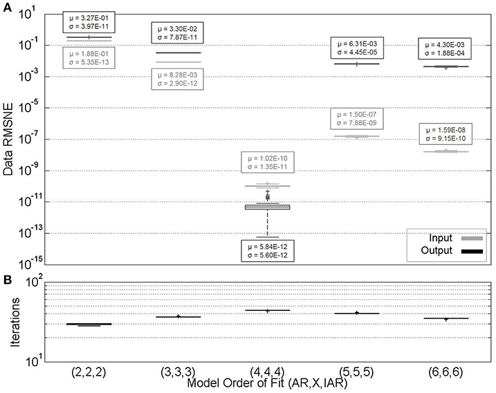
Figure 7. (A) Measurement estimate convergence for varying model order fits for simulated dataset. (B) Iterations to convergence.

From Figure 6 it is clear that parameter estimates are very accurate when correct model order is selected, and less accurate when lower model orders are selected. Larger model orders (converging in 35 and 40 iterations) have non-zero parameter estimates at all time lags, and fail to identify the proper parameter estimates. In Figure 7, however, the results of data RMSNE calculations are presented in a similar format to Figures 3B, 4B, 5B. For input data, it can be seen that there does not appear to be an appreciable difference in measurement estimates for higher order models compared to lower, despite different parameter estimates. However, output data is more accurately reconstructed in over-parameterized systems. In real systems, a “correct” model order is not accessible. Together, these observations regarding parameter and dataset estimates highlight the importance of consistent, as opposed to necessarily “correct” model order selection as a system is monitored over time. This is particularly important if regression parameters are being monitored as indicators of system change. However, these observations also suggest that dataset reconstruction may occur with safe (i.e., large) estimates of system model orders when they are unknown.

Variable Model Order—Experimental

The aim of this section is to investigate the convergence behavior of the algorithm with variable model orders. Here, we have only considered one simulation for each model order grouping (each which corresponds to a data point on Figures 8, 9). In Figures 8 (output data) and 9 (input data), the size of a plotted point is inversely proportional to the RMSNE of the converged Kalman estimated data values. The shade distribution of the plotted points can be likened to a histogram of the iterations to convergence when compared with other points, with four distinct shades corresponding to “bins” of size 60. So, for example, the (2, 2, 2) point has the lightest shade, and corresponds to a set of model orders that converged in the algorithm in 60 iterations or less. Finally, the numbers above and/or below select points on the figures correspond to the maximum, minimum, and quartile iteration or RMSNE values obtained in the analysis. For example, the (4, 2, 4) point converged in 210 iterations, tied for the most of any model order grouping. As another example, point (2, 6, 4) resulted in one of the lowest RMSNE values of any model order considered. In all cases, 20% of data was randomly missing from the experimental dataset.

FIGURE 8

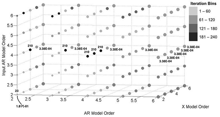
Figure 8. Convergence behavior of output data estimates with varying model orders for simulated dataset.

FIGURE 9

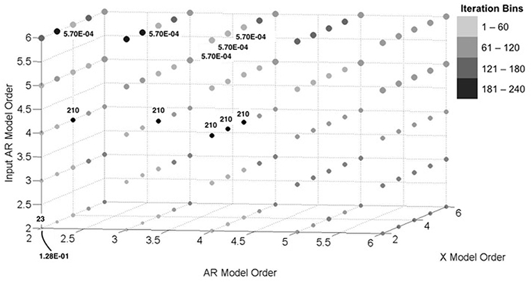
Figure 9. Convergence behavior of input data estimates with varying model orders for simulated dataset.

In many ways, aspects of this figure correspond well with previous observations. We noted in Section Variable Missing Data Pattern—Experimental that the X parameters were lower in magnitude than the AR or input AR. This implies that the ARX model may in fact be dominated by the AR portion for these particular datasets; sure enough, in Figures 8, 9, we tend to see the largest accuracy with high-order AR and input AR model orders, respectively. Furthermore, while convergence is relatively quick, lower accuracy at lower model orders is observed across the board, which likely confirms the earlier notion that structural vibrations may be described specifically with high-order AR processes.

Variable Noise—Simulated

The aim of this section is to investigate the effect of the signal-to-noise ratios in parameter identification. Datasets were simulated corresponding to the procedure in Section Simulated Data, and noise levels in Figure 10 were normally distributed with variances the indicated percentages of the initial signal values. In all cases, 20% data was randomly missing, and box plot shade conventions are the same as in Section Variable Missing Data Pattern—Experimental.

FIGURE 10

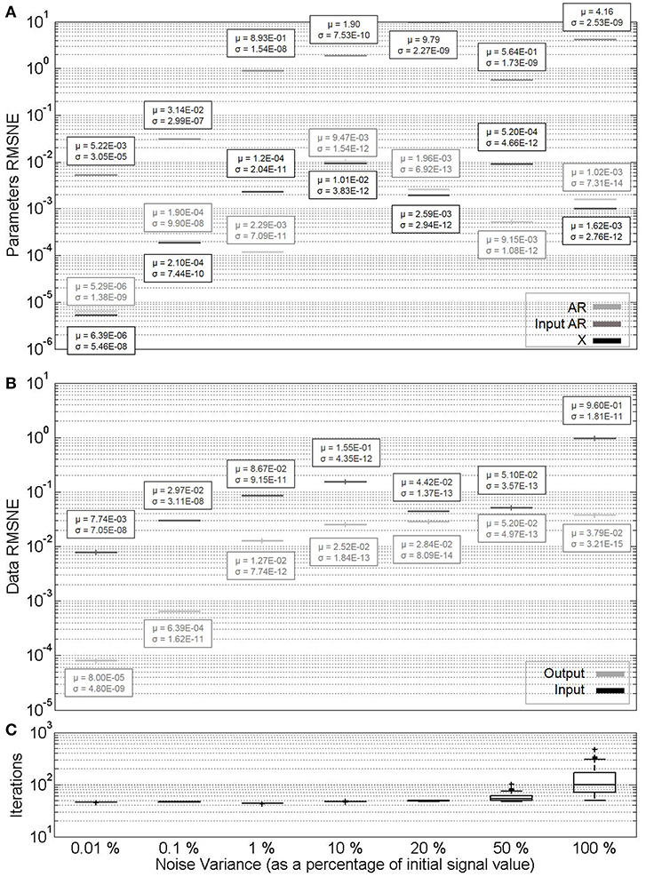
Figure 10. (A) Parameter estimate convergence for different noise levels in simulated datasets with 20% missingness. (B) Measurement estimate convergence. (C) Iterations to convergence.

It can be seen from Figure 10 that with the exception of very low noise increasing percentages of noise do not seem to significantly affect parameter estimates. This is due to the characteristics of the Kalman filter mentioned in Section Maximum Likelihood, Expectation Maximization, and Kalman Filter. Furthermore, the number of iterations do not typically significantly increase as noise levels do, though their variability does to some extent. Finally, it may be noted that data estimates errors increase exponentially with the noise from low levels, then stabilize at higher noise variance. This effect is expectedly more drastic for the output data, as it is affected by both its own noise, as well as that in the input.

Model Type: ARX vs. AR—Simulated

Finally, the performance of the algorithm for parameter identification of ARX models is compared to that of AR models. Datasets are simulated according to the procedure of Section Simulated Data, which in the case of AR does not require X or input AR parameters (third and fourth columns of Table 1). Also of note is the increasing percentages of missing data across the horizontal axes of Figures 11, 12. In all cases, no noise was included in the simulation.

FIGURE 11

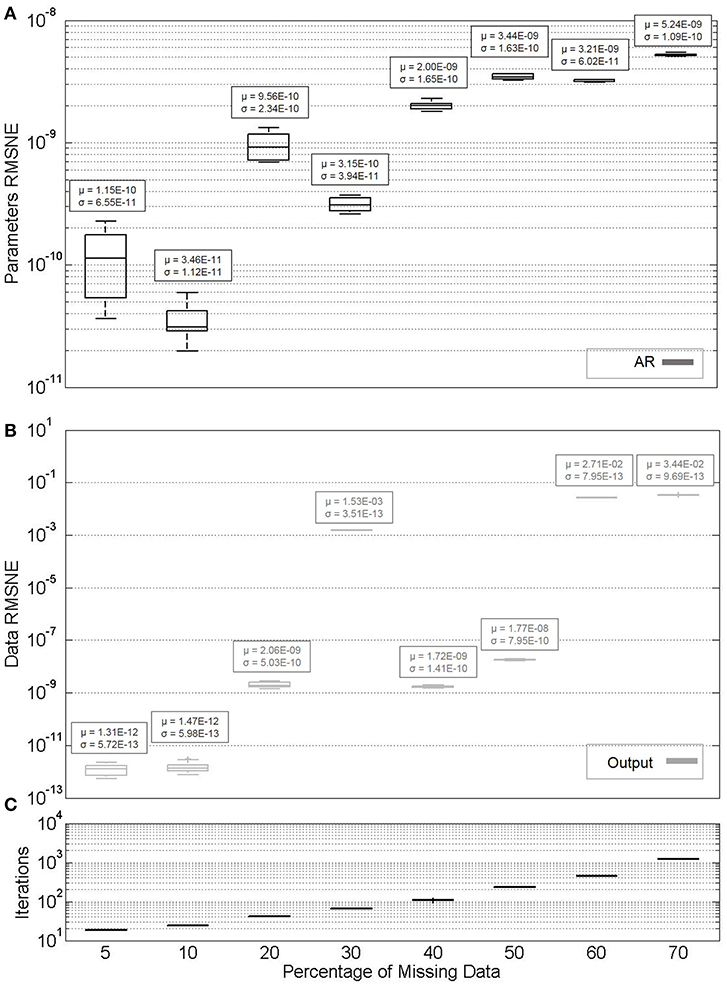
Figure 11. (A) Parameter estimate convergence for simulated AR models with varying percentages of missing data. (B) Measurement estimate convergence. (C) Iterations to convergence.

FIGURE 12

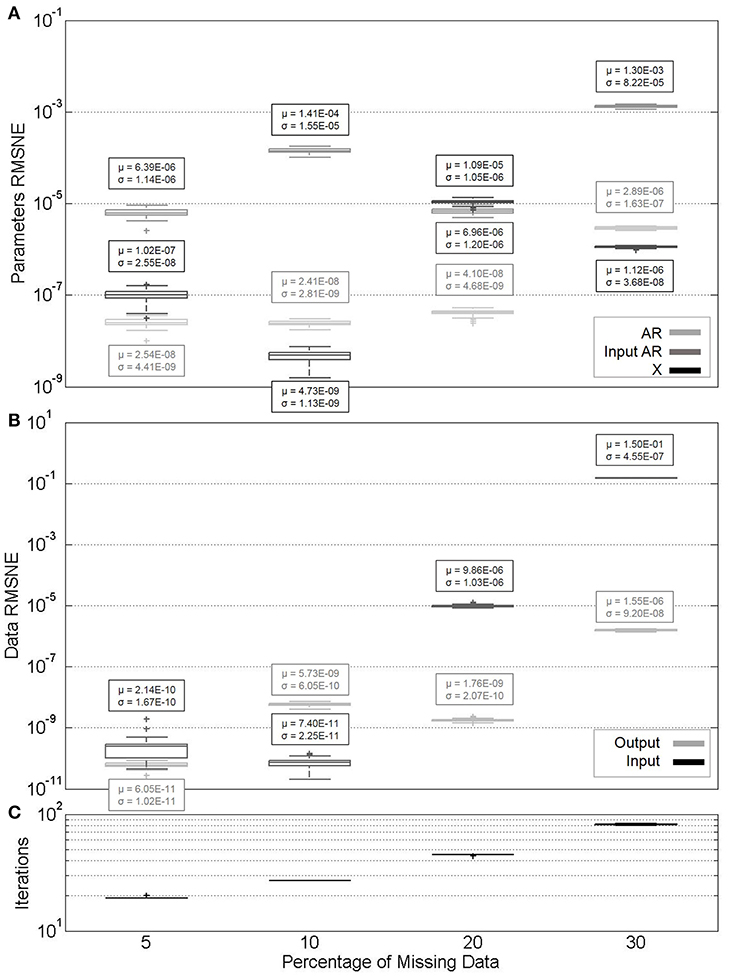
Figure 12. (A) Parameter estimate convergence for simulated ARX models with varying percentages of missing data. (B) Measurement estimate convergence. (C) Iterations to convergence.

In addition to that shown in the figure, the algorithm was also performed for the simulated case where no observations were missing. Both mean and standard deviation of RMSNE values for input AR parameters and output data is zero (it is for this reason that the results are not included in Figure 11). This result is reached in an average of 18 iterations with a standard deviation of 0.483.

Similarly, for the zero missingness ARX model input data, mean and standard deviation of RMSNE values are 7.57e–16 and 8.23e–16, respectively. For output data, mean and standard deviation are 1e–16 and 1e–15, respectively. Mean and standard deviation of X parameter RMSNE values are 1.29e–11 and 1.46e–11, respectively; for input AR parameter RMSNE values, 6.81e–15 and 6.8e–14, respectively; and for AR parameter RMSNE values, 1.76e–13 and 2.11e–13, respectively.

If the AR parameters are compared between Figures 11, 12, it can be seen that they are estimated more accurately for the purely AR model, as opposed to ARX. This may be a function of the model type selected for this particular system. Similar to experimental datasets, the X parameters are again evaluated with generally a lower degree of accuracy. It is worth noting that if ARX identification in Figure 12 is compared to that in Figure 3 (random missingness), simulated datasets' parameters are generally estimated at a higher degree of accuracy when compared to real datasets, at similar percentages of missingness. However, in the case of simulated datasets, the algorithm becomes impractically slow at higher percentages of missing data, and there is generally more variability in the estimates.

Conclusions

In this paper, an algorithm was proposed to identify parameters of both ARX and AR models fit to datasets with missing observations. This algorithm joins a relatively minor list of those dedicated to regression models, and more specifically ARX models, subject to missing observations, and presents important modifications to the state vector considered in the presented state-space model. The EM algorithm in conjunction with the Kalman filter is used for MLE of parameters and reconstruction. The effects of varying percentage of missing data; pattern of missing data; improper model order selection; variable AR, X, and input AR model order; noise level; and model type (ARX vs. AR) on the speed of convergence and accuracy of both parameter and completed dataset estimates was investigated. Favorable conditions for accurate parameter estimation include lower percentages of missing data, parameters of similar magnitude with one another, and selected model orders similar to those true to the dataset. Favorable conditions for dataset reconstruction include random and periodic missing data patterns, lower percentages of missing data, and proper model order selection. The algorithm is particularly robust to varied noise levels, an effect of the use of the Kalman filter.

Future research in relation to this work should further formalize the relationships that are apparent in this work. Boxplots in this work were concerned with evaluating the effect of changing initial parameter guesses; future work should explore the effects of consistent initial guesses, but variable missingness data indices. Additionally, the effect of the parameter values themselves on estimation accuracy should be further explored. An investigation should also be conducted into features of the converged ML statistical parameters that may be extracted to further evaluate the effectiveness of the algorithm, and different convergence criteria should be explored. Finally, alternative missing data patterns may be explored, including removing data from only one of the output or input at a time.

Author Contributions

Simulations, writing, and revision were carried out by both MH and SP, with additional writing and revision contributions from NG.

Funding

Research funding is partially provided by the National Science Foundation through Grant No. CMMI-1351537 by the Hazard Mitigation and Structural Engineering program, and by a grant from the Commonwealth of Pennsylvania, Department of Community and Economic Development, through the Pennsylvania Infrastructure Technology Alliance (PITA).

Conflict of Interest Statement

The authors declare that the research was conducted in the absence of any commercial or financial relationships that could be construed as a potential conflict of interest.

References

Andersen, P. (1997). Identification of Civil Engineering Structures Using Vector ARMA Models. Aalborg: Aalborg University, Department of Building Technology and Structural Engineering.

Google Scholar

Broersen, P. M., and Box, R. (2006). Time-series analysis if data are randomly missing. IEEE Transac. Instrument. Measure. 55, 79–84. doi: 10.1109/TIM.2005.861247

CrossRef Full Text | Google Scholar

Cara, F. J., Juan, J., and Alarcón, E. (2014). Estimating the modal parameters from multiple measurement setups using a joint state space model. Mech. Syst. Signal Process. 43, 171–191. doi: 10.1016/j.ymssp.2013.09.012

CrossRef Full Text | Google Scholar

Chai, T., and Draxler, R. (2014). Root mean square error (RMSE) or mean absolute error (MAE)? - Arguments against avoiding RMSE in the literature. Geosci. Model Dev. 7, 1247–1250. doi: 10.5194/gmd-7-1247-2014

CrossRef Full Text | Google Scholar

Chang, M., and Pakzad, S. N. (2013). Modified natural excitation technique for stochastic modal identification. J. Struc. Eng. 139, 1753–1762. doi: 10.1061/(ASCE)ST.1943-541X.0000559

CrossRef Full Text | Google Scholar

Chang, M., and Pakzad, S. N. (2014). Observer kalman filter identification for output-only systems using interactive structural modal identification toolsuite. J. Bridge Eng. 19:04014002. doi: 10.1061/(ASCE)BE.1943-5592.0000530

CrossRef Full Text | Google Scholar

Dempster, A. P., Laird, N. M., and Rubin, D. B. (1977). Maximum likelihood from incomplete data via the EM algorithm. J. R. Stat. Soc. Series B. 39, 1–38. doi: 10.1111/j.2517-6161.1977.tb01600.x

CrossRef Full Text | Google Scholar

Digalakis, V., Rohlicek, J. R., and Ostendorf, M. (1993). ML estimation of a stochastic linear system with the EM algorithm and its application to speech recognition. IEEE Transac. Speech Audio Process. 1, 431–442. doi: 10.1109/89.242489

CrossRef Full Text | Google Scholar

Ding, F., Liu, G., and Liu, X. P. (2011). Parameter estimation with scarce measurements. Automatica 47, 1646–1655. doi: 10.1016/j.automatica.2011.05.007

CrossRef Full Text | Google Scholar

Dorvash, S., and Pakzad, S. N. (2012). Stochastic iterative modal identification algorithm and application in wireless sensor networks. Struc. Control Health Monitor. 20, 1121–1137. doi: 10.1002/stc.1521

CrossRef Full Text | Google Scholar

Dorvash, S., Pakzad, S. N., and Cheng, L. (2013). An iterative modal identification algorithm for structural health monitoring using wireless sensor networks. Earthquake Spectra 29, 339–365. doi: 10.1193/1.4000133

CrossRef Full Text | Google Scholar

Dorvash, S., Pakzad, S. N., LaCrosse, E. L., Ricles, J. M., and Hodgson, I. C. (2015). Localized damage detection algorithm and implementation on a large-scale steel beam-to-column moment connection. Earthquake Spectra 31, 1543–1566. doi: 10.1193/031613EQS069M

CrossRef Full Text | Google Scholar

Dunsmuir, W., and Robinson, P. (1981). Estimation of time series models in the presence of missing data. J. Am. Stat. Assoc. 76, 560–568. doi: 10.1080/01621459.1981.10477687

CrossRef Full Text | Google Scholar

Grossmann, C., Jones, C. N., and Morari, M. (2009). “System identification with missing data via nuclear norm regularization,” in 2009 European Control Conference (EEC) (Budapest: IEEE), 448–453.

Google Scholar

Gul, M., and Catbas, F. N. (2009). Statistical pattern recognition for Structural Health Monitoring using time series modeling: theory and experimental verifications. Mech. Syst. Signal Process. 23, 2192–2204. doi: 10.1016/j.ymssp.2009.02.013

CrossRef Full Text | Google Scholar

Harvey, A., and Phillips, G. (1979). Maximum likelihood estimation of regression models with autoregressive-moving average disturbances. Biometrika 66:49. doi: 10.2307/2335241

CrossRef Full Text | Google Scholar

Harvey, A., and Pierse, R. (1984). Estimating missing observations in economic time series. J. Am. Stat. Assoc. 79, 125–131. doi: 10.1080/01621459.1984.10477074

CrossRef Full Text | Google Scholar

He, X., and De Roeck, G. (1997). System identification of mechanical structures by a high-order multivariate autoregressive model. Comp. Struc. 64, 341–351. doi: 10.1016/S0045-7949(96)00126-5

CrossRef Full Text | Google Scholar

Horner, M., and Pakzad, S. N. (2016a). “Parameter estimation for ARX models with missing data,” in Proceedings of the Fifth International Symposium on Life-Cycle Engineering (Bethlehem, PA).

Horner, M., and Pakzad, S. N. (2016b). Structural damage detection through vibrational feature analysis with missing data. Dyn. Civil Struc. 2, 23–30. doi: 10.1007/978-3-319-29751-4_4

CrossRef Full Text | Google Scholar

Huang, C. (2001). Structural identification from ambient vibration measurement using the multivariate AR Model. J. Sound Vibration 241, 337–359. doi: 10.1006/jsvi.2000.3302

CrossRef Full Text | Google Scholar

Isaksson, A. J. (1993). Identification of ARX-models subject to missing data. IEEE Transac. Automatic Control 38, 813–819. doi: 10.1109/9.277253

CrossRef Full Text | Google Scholar

James, G. H. III, Carne, T. G., and Lauffer, J. P. (1993). The Natural Excitation Technique (NExT) for Modal Parameter Extraction From Operating Wind Turbines. Albuquerque, NM: Sandia National Laboratories.

Jones, R. H. (1980). Maximum likelihood fitting of ARMA models to time series with missing observations. Technometrics 22, 389–395. doi: 10.1080/00401706.1980.10486171

CrossRef Full Text | Google Scholar

Juang, J.-N., and Pappa, R. S. (1985). An eigensystem realizaiton algorithm for modal parameter identification and model reduction. J. Guidance Control Dyn. 8, 620–627. doi: 10.2514/3.20031

CrossRef Full Text | Google Scholar

Kalman, R. E. (1960). A new approach to linear filtering and prediction problems. J. Basic Eng. 82, 35–45. doi: 10.1115/1.3662552

CrossRef Full Text | Google Scholar

Kolenikov, S. (2003). AR(1) Process With Missing Data. Available online at: https://www.researchgate.net/profile/Stanislav_Kolenikov/publication/267409126_AR1_process_with_missing_data/links/54c015190cf28a6324a0f6fd/AR1-process-with-missing-data.pdf

Google Scholar

Kullaa, J. (2009). Eliminating environmental or operational influences in structural health monitoring using the missing data analysis. J. Intell. Mater. Syst. Struc. 20, 1381–1390. doi: 10.1177/1045389X08096050

CrossRef Full Text | Google Scholar

Little, R. J., and Rubin, D. B. (2002). Statistical Analysis with Missing Data (Vol. 2). Hoboken, NJ: John Wiley & Sons, Inc.

Mader, W., Linke, Y., Mader, M., Sommerlade, L., Timmer, J., and Schelter, B. (2014). A numerically efficient implementation of the expectation maximization algorithm for state space models. Appl. Mathematics Comput. 241, 222–232. doi: 10.1016/j.amc.2014.05.021

CrossRef Full Text | Google Scholar

Matarazzo, T. J., and Pakzad, S. N. (2014). Modal identification of golden gate bridge using pseudo mobile sensing data with STRIDE. Proc. Soc. Exp. Mech. IMAC XXXII 4, 293–298. doi: 10.1007/978-3-319-04546-7_33

CrossRef Full Text | Google Scholar

Matarazzo, T. J., and Pakzad, S. N. (2015). STRIDE for structural identification using expectation maximization: iterative output-only method for modal identification. J. Eng. Mech. 142:04015109. doi: 10.1061/(ASCE)EM.1943-7889.0000951

CrossRef Full Text | Google Scholar

Matarazzo, T. J., and Pakzad, S. N. (2016a). Sensitivity metrics for maximum likelihood system identification. ASCE ASME J. Risk Uncertainty Eng. Syst. Part A Civil Eng. 2:B4015002. doi: 10.1061/AJRUA6.0000832

CrossRef Full Text | Google Scholar

Matarazzo, T. J., and Pakzad, S. N. (2016b). Structural identification for mobile sensing with missing observations. J. Eng. Mech. 142:04016021. doi: 10.1061/(ASCE)EM.1943-7889.0001046

CrossRef Full Text | Google Scholar

Matarazzo, T. J., and Pakzad, S. N. (2016c). Truncated physical model for dynamic sensor networks with applications in high-resolution mobile sensing and BIGDATA. J. Eng. Mech. 142:04016019. doi: 10.1061/(ASCE)EM.1943-7889.0001022

CrossRef Full Text | Google Scholar

McGiffin, P., and Murthy, D. (1980). Parameter estimation for auto-regressive systems with missing observations. Int. J. Syst. Sci. 11, 1021–1034. doi: 10.1080/00207728008967071

CrossRef Full Text | Google Scholar

McGiffin, P., and Murthy, D. (1981). Parameter Estimation for auto-regressive systems with missing observations–Part II. Int. J. Syst. Sci. 12, 657–663. doi: 10.1080/00207728108963775

CrossRef Full Text | Google Scholar

Nagarajaiah, S., and Chen, B. (2016). Output only structural modal identification using matrix pencil method. Struc. Monitoring Maintenance 3, 395–406. doi: 10.12989/smm.2016.3.4.395

CrossRef Full Text | Google Scholar

Naranjo, A. H. (2007). State-Space Models with Exogenous Variables and Missing Data (Ph.D. thesis). University of Florida, Gainesville, FL, United States.

Google Scholar

Nigro, M., and Pakzad, S. (2014). Localized structural damage detection: a change point analysis. Computer Aided Civil Infrastructure Eng. 29, 416–432. doi: 10.1111/mice.12059

CrossRef Full Text | Google Scholar

Nozari, A., Behmanesh, I., Yousefianmoghadam, S., Moaveni, B., and Stavridis, A. (2017). Effects of variability in ambient vibration data on model updating and damage identification of a 10-story building. Eng. Struc. 151, 540–553. doi: 10.1016/j.engstruct.2017.08.044

CrossRef Full Text | Google Scholar

Pakzad, S. N., Rocha, G. V., and Yu, B. (2011). Distributed modal identification using restricted auto regressive models. Int. J. Syst. Sci. 42, 1473–1489. doi: 10.1080/00207721.2011.563875

CrossRef Full Text | Google Scholar

Sadeghi Eshkevari, S., and Pakzad, S. (2019). Signal Reconstruction from Mobile Sensors Network using Matrix Completion Approach. Dynamics of Civil Structures. Cham: Springer.

Sargan, J., and Drettakis, E. (1974). Missing Data in an Autoregressive Model. Int. Econ. Rev. 15, 39–58. doi: 10.2307/2526087

CrossRef Full Text | Google Scholar

Shahidi, S. G., Nigro, M. B., Pakzad, S. N., and Pan, Y. (2015). Structural damage detection and localisation using multivariate regression models and two-sample control statistics. Struc. Infrastructure Eng. 11, 1277–1293. doi: 10.1080/15732479.2014.949277

CrossRef Full Text | Google Scholar

Shahidi, S. G., and Pakzad, S. N. (2014a). Effect of measurement noise and excitation on Generalized Response Surface Model Updating. Eng. Struc. 75, 51–62. doi: 10.1016/j.engstruct.2014.05.033

CrossRef Full Text | Google Scholar

Shahidi, S. G., and Pakzad, S. N. (2014b). Generalized response surface model updataing using time domain data. J. Struc. Eng. 140:4014001. doi: 10.1061/(ASCE)ST.1943-541X.0000915

CrossRef Full Text

Shi, Y., and Fang, H. (2010). Kalman filter-based identification for systems with randomly missing measurements in a network environment. Int. J. Control 83, 538–551. doi: 10.1080/00207170903273987

CrossRef Full Text | Google Scholar

Shumway, R., and Stoffer, D. (1982). An approach to time series smoothing and forecasting using the EM algorithm. J. Time Series Analysis 3, 253–264. doi: 10.1111/j.1467-9892.1982.tb00349.x

CrossRef Full Text | Google Scholar

Shumway, R. H., and Stoffer, D. S. (2000). Time Series Analysis and Its Applications: With R Examples. New York, NY: Springer.

Google Scholar

Sohn, H., Farrar, C. R., Hunter, N. F., and Worden, K. (2001). Structural health monitoring using statistical pattern recognition techniques. J. Dyn. Syst. Measure. Control 123, 706–711. doi: 10.1115/1.1410933

CrossRef Full Text | Google Scholar

Song, M., Yousefianmoghadam, S., Mohammadi, M.-E., Moaveni, B., Stavridis, A., and Wood, R. L. (2017). An application of finite element model updating for damage assessment of a two-story reinforced concrete building and comparison with lidar. Struc. Health Monitor. 17, 1129–1150. doi: 10.1177/1475921717737970

CrossRef Full Text | Google Scholar

Wallin, R., and Hansson, A. (2014). Maximum likelihood estimation of linear SISO models subject to missing output data and missing input data. Int. J. Control 87, 1–11. doi: 10.1080/00207179.2014.913346

CrossRef Full Text | Google Scholar

Wallin, R., and Isaksson, A. J. (2000). “An iterative method for identification of ARX models from incomplete data,” in Proceedings of the 39th IEEE Conference on Decision and Control (Sydney, NSW), 203–208.

Google Scholar

Wallin, R., and Isaksson, A. J. (2002). Multiple Optima in Identification of ARX models subject to missing data. EURASIP J. Adv. Signal Process. 2002, 1–8. doi: 10.1155/S1110865702000379

CrossRef Full Text | Google Scholar

Yao, R., and Pakzad, S. N. (2012). Autoregressive statistical pattern recognition algorithms for damage detection in civil structures. Mech. Syst. Signal Process. 31, 355–368. doi: 10.1016/j.ymssp.2012.02.014

CrossRef Full Text | Google Scholar

Yousefianmoghadam, S., Stavridis, A., Behmanesh, I., Moaveni, B., and Nozari, A. (2016). “System identification and modeling of a 100-year-old RC warehouse dynamically tested at several damage states,” in Proceedings of 1st International Conference on Natural Hazards & Infrastructure (Chania).

Google Scholar

Zgheib, R., Fleury, G., and Lahalle, E. (2006). New Fast Algorithm for Simulatneous Identification and Optimal Reconstruction of Non Stationary AR Processes With Missing Observations. Grand Teton National Park, WY: Digital Signal Processing Workshop, 371.

Google Scholar