Output-Only Vibration-Based Monitoring of Civil Infrastructure via Sub-Nyquist/Compressive Measurements Supporting Reduced Wireless Data Transmission

Introduction

In recent years, monitoring schemes have roved their worth in terms of the potential for smart operation and maintenance of civil structures (Farrar and Worden, 2012). When further coupled with the concept of the Value of Information, monitoring of structures serves as a direct tool for informing decision support on the life cycle management of structural assets. In this context, operational modal analysis (OMA) involves an efficient monitoring modality in large scale structural systems, as it is typically enabled by low cost acceleration sensors, allowing for a long-term or permanent system supervision (Limongelli et al., 2016). Due to the difficulty involved in the measurement of operating loads, OMA relies on output-only information for extraction of dynamic properties of systems that are typically subjected to low-amplitude operational loads (e.g., due to wind traffic, etc.) (Brincker and Ventura, 2015). For the common case of linear systems, such properties include the modal characteristics of the structure (e.g., natural frequencies, damping and mode shapes). Since no explicit loading information is assumed available, output-only techniques commonly assume ambient conditions corresponding to a flat spectrum over a wide range of frequencies (i.e., a white noise excitation assumption). Such techniques are shown to perform well, even under the challenge of varying environmental and operational conditions (Reynders et al., 2013; Shi et al., 2016; Avendaño-Valencia et al., 2017) while the extracted modal structural properties may be then exploited for a variety of tasks including condition assessment, design verification, structural health monitoring (SHM) and, ultimately, residual life prediction of civil structures (Straub et al., 2017). Still, OMA has been mostly demonstrated for use with tethered sensing configurations.

Wireless sensor networks (WSNs) offer a low-cost and easily deployable alternative to tethered (wired) acceleration sensors that is particularly attractive for large structures featuring locations of reduced accessibility (Lynch, 2007). The “smart” feature of most such wireless platforms, allowing for local processing at the wireless senor (node) level, has been exploited for decentralized autonomous monitoring solutions (Nagayama et al., 2009). Nonetheless, WSNs have so far not enjoyed widespread adoption into practice, largely owing to their limited wireless transmission bandwidth and the maintenance costs related to frequent battery replacement (Klis and Chatzi, 2016a; Gkoktsi and Giaralis, 2019).

In order to extend the self-sustainability of the nodes, and to reduce the power allocated for transmission, compressive sensing (CS) techniques have been explored, with Bao et al. (2010) and O'Connor et al. (2013), leading developments in this field, with applications on actual road bridges. CS samples at random non-uniform in time rates, resulting in equivalent sampling below the Nyquist rate. In a nutshell, CS asserts that a discrete-time finite length signal (e.g., an analog response acceleration signal uniformly sampled in time) can be recovered, with high probability, from a relatively small number of randomly acquired samples/measurements in time, by solving an underdetermined system of linear equations (Candès and Tao, 2006; Donoho, 2006). Importantly, the number of random (compressed) measurements required for a faithful signal recovery depends on the “sparsity” of the acquired signal with respect to some pre-specified vector basis, such as the discrete Fourier transform (DFT) basis used for representation of vectors in the Fourier/frequency domain. Specifically, a K-sparse/compressible signal features K expansion coefficients on a given basis with values larger than a relatively low threshold; the smaller K is, the sparser the signal is, and thus the fewer random measurements are required for its sparse recovery (i.e., estimation of the K significant expansion coefficients) within the CS framework. In this regard, all algorithms for sparse signal recovery necessitate an assumption of signal sparsity (Vaswani and Zhan, 2016), which is a priori unknown and is adversely affected by signal noise. Further, much research work has been devoted in constructing sparsifying bases or, more generally, sparsifying dictionaries tailored for different applications, such as image denoising (Razaviyayn et al., 2014), video sensing (Eslani et al., 2014), and ultrasonic non-destructive damage detection (Fuentes et al., 2019).

In this setting, O'Connor et al. (2014) were the first to deploy customized CS-based wireless sensors in a long-term monitoring field application for an overpass in MI, USA. By randomly triggering in time conventional ADC units, non-uniform in time compressed acceleration response signals were acquired. Sparse recovery assuming a DFT expansion basis, as well as an empirically specified level of sparsity was applied to the compressed data to estimate the response acceleration power spectral density (PSD) matrix. The latter matrix was used in conjunction with the standard frequency domain decomposition (FDD) algorithm to extract mode shapes and natural frequencies within OMA. Yang and Nagarajaiah (2015) and Park et al. (2014) contributed two significantly different approaches for mode shape estimation from CS-based non-uniform in time random sampling of structural vibration time-histories at sub-Nyquist rates. In Yang and Nagarajaiah (2015) mode shape estimation relies on modal structural responses obtained by application of blind source separation directly to the compressed measurements of structural response signals. Sparse signal recovery (reconstruction) in the time-domain is next applied to each compressed modal response vector to retrieve the underlying structural natural frequencies and modal damping ratios. In Park et al. (2014) mode shapes are obtained by means of a singular value decomposition-based algorithm applied directly to response acceleration compressed measurements, without taking any reconstruction step, under the assumption of noiseless undamped free vibration structural response signals (i.e., multi-tone signal model).

The standard approach to CS-based signal recovery relies on l₁-norm minimization and solution of the so-called Basis Pursuit De-Noising problem (BPDN). This approach is typically adopted in CS implementations in OMA applications using wireless sensors (O'Connor et al., 2014; Zou et al., 2015). In enhancing the BPDN approach, Klis and Chatzi (2016b) utilize its re-weighted variant, known as the re-weighted Basis Pursuit De-Noising problem (rwBPDN), also known as the l₁-analysis problem (Becker et al., 2011). The resulting Spectro-temporal CS (STCS) scheme leads to improved time-domain signal recovery with respect to the standard BPDN approach. Furthermore, in order to alleviate the heuristic a priori assumption on sparsity Klis and Chatzi (2016a) initially exploit the concept of a leading node, i.e., a (typically) tethered node which is permanently logging at higher sampling rates, and forms part of a Hybrid Sensor Network (HSN). The latter forms a compilation of primarily wireless and a minimal number of tethered sensors. In this way the signal support, on the basis of which the recovery is performed, is narrowed, which results in reduced transmission costs. In later work (Klis and Chatzi, 2016b) the leading node requirement is removed, with wireless sensors transmitting partial temporal information and a selected part of the spectral information in a two way communication with the server (central node). Sparse signal recovery is again enabled via solution of the rwBPDN problem. The recovered signals may then serve as input for any standard output-only modal identification algorithm for OMA. As signal reconstruction is a main target of this approach, it is particularly attractive for use with time domain-based identification methods, such as approaches based on Auto-regressive models, subspace identification algorithms, or real-time tracking using Kalman filters. The proposed scheme has been validated on synthetic simulations generated for a benchmark four-story frame structure of the American Society of Civil Engineers, as well as data from operating structures.

Aiming to circumvent the signal sparsity requirement for the identification of modal characteristics (natural frequencies and modal shapes) from sub-Nyquist sampled response acceleration data, Gkoktsi and Giaralis (2017), Gkoktsi and Giaralis (2019) developed an alternative to the former CS-based approaches. The latter approach couples the sub-Nyquist non-uniform-in-time deterministic multi-coset sampling strategy (Venkataramani and Bresler, 2001), with a Power Spectrum Blind Sampling (PSBS) technique (Ariananda and Leus, 2012; Tausiesakul and González-Prelcic, 2013) extended to the multi-channel case by Gkoktsi et al. (2015) to estimate the response acceleration PSD matrix (second order statistics) from correlation sequences of the sub-Nyquist measurements. Ultimately, the considered PSBS approach derives structural modal properties by application of the FDD algorithm to the estimated PSD matrix without response acceleration signal recovery in the time domain and without making an a priori assumption on signal sparsity in the DFT or in any other domain (Gkoktsi and Giaralis, 2017). In doing so, measured response signals are assumed as stationary correlated stochastic processes in alignment with OMA theory (Brincker and Ventura, 2015). In this respect, the PSBS approach does not return the time-histories of acceleration response signals but, on the positive side, it is purely signal agnostic in terms of signal structure in the frequency domain and, therefore, indifferent to signal sparsity attributes and/or to additive noise. In this regard, it was shown that the PSBS approach achieves quality mode shape extraction and robust modal strain-based damage detection from response acceleration measurements corrupted by additive noise (Gkoktsi et al., 2016) at rates as low as 80% below Nyquist leading to significant energy consumption gains in wireless sensors (Gkoktsi and Giaralis, 2019).

Previously, the PSBS approach has been compared to standard BPDN CS-based approach in terms of quality mode shape extraction (Gkoktsi and Giaralis, 2017). Herein, we comparatively assess the PSBS-based scheme (Gkoktsi and Giaralis, 2017, 2019) and the STCS approach (Klis and Chatzi, 2016a,b) in an effort to demonstrate their readiness levels for output-only modal identification supported by low-power wireless sensors which is the first step toward cost-effective SHM. The strengths and limitations of each approach are elaborated upon, with a comparison in terms of data compression, potential for modal identification, and, for the case of STCS, on time-domain signal recovery. In order to validate the presented tools, field data from large scale structures are utilized, namely acceleration response time-histories from an operating on-shore wind turbine as well as from a highway overpass open to traffic. For the second structure, estimated battery lifetime gains at the sensor node level are provided achieved by power consumption savings from reduced wireless data transmission.

Methodological Framework

Spectro-Temporal Compressive Sensing (STCS) Approach via rwBPDN

Spectro-Temporal Compressive Sensing (STCS) relies on the formulation of the missing data estimation problem (Candès and Romberg, 2007; Becker et al., 2011; Candès and Plan, 2011). Let us assume a signal recorded by sensor i, comprising N samples. The missing data estimation problem is formulated as:

$\begin{array}{ll}{\text{y}}_i=\text{S}{\text{x}}_i& (1)\end{array}$

where ${\text{y}}_i={\left[y_{1i},y_{2i},\dots ,y_{Mi}\right]}^T\in {ℝ}^M$is the measured signal of partial (incomplete) observations, comprising a dimension M < N, and S ∈ ℝ^{M × N}is a zero-one selection matrix, known a-priori. The goal of the missing data estimation problem is to recover the original full signal x_i given the incomplete observations y_iand the selection matrix S.

As demonstrated in Klis and Chatzi (2016b) structural response signals admit a sparse representation via a Discrete Fourier Transform (DFT) orthonormal basis, A ∈ ℂ^{N × N}, according to the following equation:

$\begin{array}{ll}{\text{x}}_i=\text{A}{\text{c}}_i,\text{where }{\text{A}}_{i,l}=\frac{1}{\sqrt{N}}{e}^{-j2\pi i\frac{l}{N}}& (2)\end{array}$

where ${\text{c}}_i={\left[c_{1i},c_{2i},\dots ,c_{Ni}\right]}^T\in {ℝ}^N$comprises the coefficient vector. Via substitution of equation (2) into equation the observations vector y_i may be recovered on the basis of a finite number of c_isparse coefficients, as follows:

$\begin{array}{ll}{\text{y}}_i=\text{S}\text{A}{\text{c}}_i& (3)\end{array}$

When the vector of observations y_iis incomplete, as is the case for missing data, equation (3) comprises an ill-conditioned problem with multiple solutions for the coefficients vector c_i. Within the compressive sensing context however, we are interested in the solution rendering the most sparse vector c_i, for which equation (1) is fulfilled. This is recovered via solution of a non-deterministic polynomial time-Hard (NP-Hard) combinatorial problem:

$\begin{array}{ll}{\displaystyle \underset{{\text{c}}_i}{\text{arg min }}}{\Vert {\text{c}}_i\Vert }_0\text{\hspace{1em}subject to }{\text{y}}_i=\text{S}\text{A}{\text{c}}_i& (4)\end{array}$

As the formulation of equation (4) is non-trivial to solve, Candès and Romberg (2007) concluded that solving a relaxed || · ||₁ convex optimization problem, known as a basis pursuit problem, is equivalent to solving the original || · ||₀NP-Hard combinatorial problem, given that an appropriate condition—the so-called Restricted Isometry Property (RIP)—holds. The basis pursuit problem is expressed as:

$\begin{array}{ll}{\displaystyle \underset{{\text{c}}_i}{\text{arg min }}}{\Vert {\text{c}}_i\Vert }_1\text{\hspace{1em}subject to }{\text{y}}_i=\text{S}\text{A}{\text{c}}_i& (5)\end{array}$

The formulation of equation offers a significant reduction in terms of computational toll, while guaranteeing that the original response signal x_i may be fully recovered, provided that the K-RIP condition is satisfied by matrix SA. For each positive integer K, we may define the isometry constant δ_K of matrix SA as the smallest integer ensuring that the following K-RIP condition holds for all K-sparse vectors:

$\begin{array}{ll}(1-{\delta }_K)\Vert {\text{c}}_i{\Vert }_2^2\le \Vert \text{S}\text{A}{\text{c}}_i{\Vert }_2^2\le (1+{\delta }_K)\Vert {\text{c}}_i{\Vert }_2^2& (6)\end{array}$

According to Candès et al. (2006) if ${\delta }_{2K}<\sqrt{2}-1$ then a solution to (5) will also satisfy the original problem (4) with a good quality of approximation.

However, observations stemming from acquisition via sensor nodes, as is typical for SHM measurements, will be corrupted with noise. In this case, the original problem becomes

$\begin{array}{ll}{\text{y}}_i=\text{S}\text{A}{\text{c}}_i+{\text{z}}_i,{\text{z}}_i\propto {N}(0,{\sigma }^2)& (7)\end{array}$

The solution to this modified problem is obtained via a convex optimization problem, known as the Basis Pursuit De-Noising problem (BPDN):

$\begin{array}{ll}{\displaystyle \underset{{\text{c}}_i}{\text{arg min }}}{\Vert \text{c}\Vert }_1\text{ subject to }{\Vert {\text{y}}_i-\text{S}\text{A}{\text{c}}_i\Vert }_2\le ϵ& (8)\end{array}$

Solution of the BPDN problem has been the main approach utilized so far in the context of CS for SHM implementations (O'Connor et al., 2014; Wang and Hong, 2015; Wang et al., 2015). Klis and Chatzi (2016b) have advanced this framework by utilizing in lace of the classical BPDN formulation, its re-weighted variant, known as the re-weighted Basis Pursuit De-Noising problem (rwBPDN) (Becker et al., 2011):

$\begin{array}{ll}{\displaystyle \underset{{\text{c}}_i}{\text{arg min }}}{\Vert \text{W}{\text{c}}_i\Vert }_1\text{ subject to }{\Vert {\text{y}}_i-\text{S}\text{A}{\text{c}}_i\Vert }_2\le ϵ& (9)\end{array}$

Key to this formulation is the weighting matrix W = diag([w₁, w₂, …, w_N]) which ensures a desired structure of the coefficient vector c_i.

The Spectro-Temporal Compressive Sensing (STCS) framework relies on solution of the rw-BPDN problem. Figure 1 illustrates the steps of STCS framework, with the actions performs locally on the node level aggregated on the left, and actions performed globally at the base station (server) level assembled on the right. As a first step, the support is determined at each node. The support of a vector is defined as the subset of non-zero components supp(Y_i) = {ω ∈ Ω : Y_i(ω) ≠ 0}. For practical implementations, this is eventually defined in terms of exceedance of a user-specified threshold ϵ : supp(Y_i, ϵ) = {ω ∈ Ω : |Y_i(ω)| > ϵ}. The selection of the support is executed for windowed frames x_ij, extracted from the original signal x_i. The formulated support U_ij, as well as its complementary set ${\text{U}}_{ij}^c$ allow the decomposition of the spectral representation of the signal, as expressed via the coefficient vector c_i, into a “noisy” and “clean” component ${\text{c}}_{ij}={\text{U}}_{ij}{\text{c}}_{ij}+{\text{U}}_{ij}^c{\text{c}}_{ij}$. The locally defined support components are eventually transmitted to the server, where the weighting matrix W_ij is formulated and the K-sparsity of the signal is determined as K_ij = ∑(U_ij).

FIGURE 1

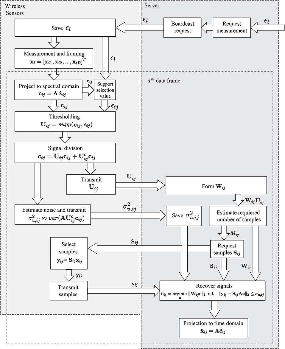
Figure 1. Flowchart of spectro-temporal compressive sensing framework (Klis and Chatzi, 2016b).

In a next step, the number of time-domain samples M_ij required for signal recovery is defined, on the basis of which the server randomly selects and transmits y_ij sub-vectors, from the j-th data frame of the i-th sensor, using a uniform distribution. For more details on this process the interested reader is referred to (Klis and Chatzi, 2016b). Upon transmission of the necessary time domain samples, along with the corresponding W_ij weighting matrix, to the server the coefficient vector is recovered as ${\widehat{\text{c}}}_{ij}=\underset{{\text{c}}_{ij}}{\text{arg min}}{\Vert {\text{W}}_{ij}{\text{c}}_{ij}\Vert }_1\text{subject to}{\Vert {\text{y}}_{ij}-{\text{S}}_{ij}\text{A}{\text{c}}_{ij}\Vert }_2\le {\sigma }_{u,ij}$. As a last step, the coefficient vector of the j-th data frame is projected back to the time domain:

$\begin{array}{ll}{\widehat{\text{x}}}_{ij}=\text{A}{\widehat{\text{c}}}_{ij}& (10)\end{array}$

Once this process has been executed for each data frame, the estimate of the full time domain signal is attained as ${\widehat{\text{x}}}_i={\left[{\widehat{\text{x}}}_{i1},{\widehat{\text{x}}}_{i2},\dots ,{\widehat{\text{x}}}_{iD}\right]}^T$ from all D sensors in the network. The solver adopted for solution of the involved rwBPDN problem is the NESTA algorithm (Nesterov, 2005; Becker et al., 2011).

The Multi-Channel Power Spectrum Blind Sampling (PSBS) Approach

The multi-channel PSBS approach for operational modal analysis developed by Gkoktsi and Giaralis (2017), Gkoktsi and Giaralis (2019) comprises the three stages delineated in Figure 2. The first stage involves low-rate (sub-Nyquist) deterministic periodic non-uniform-in-time multi-coset sampling at all D acceleration sensing nodes. In the next stage, the low-rate (compressed) measurements from all sensors are wirelessly transmitted to a server (base station) and centrally processed to obtain their cross-correlation vectors. These vectors are used to estimate (recover) the response acceleration PSD matrix by solving an overdetermined system of linear equations without invoking any signal sparsity assumption. Lastly, in stage III, the FDD algorithm is applied to the recovered PSD matrix to obtain natural frequencies and mode shapes. Notably, this centralized 3-stage forward-only approach minimizes processing and memory requirements at the node (local) level as well as wireless data communication payload within the WSN leading to low-complexity and low-energy consumption sensor nodes.

FIGURE 2

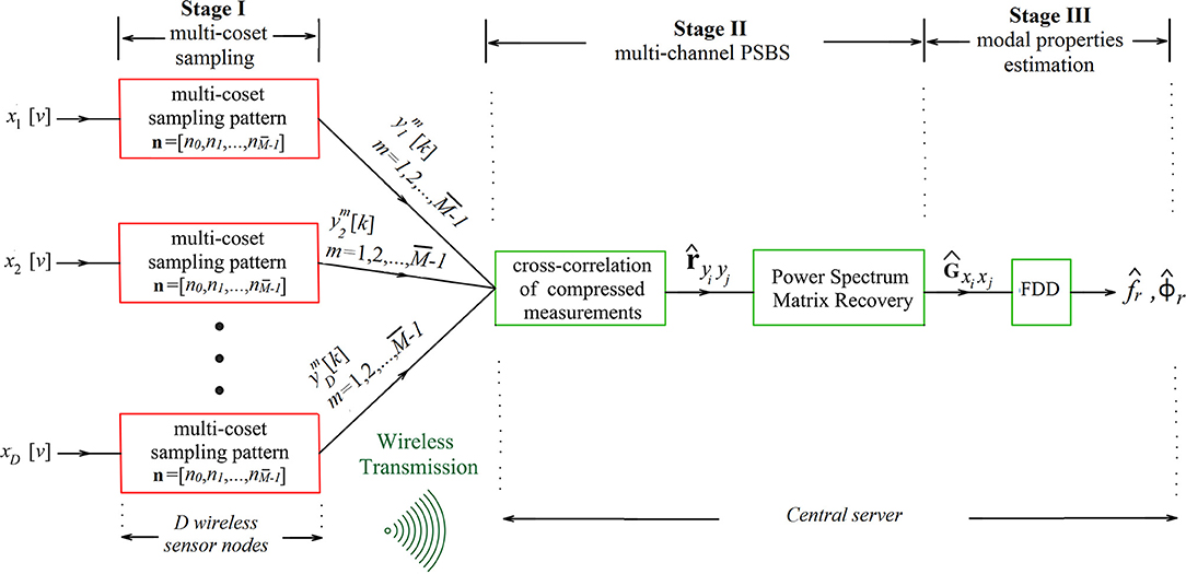
Figure 2. Flowchart of multi-channel power spectrum blind sampling approach for frequency domain OMA (see also Gkoktsi and Giaralis, 2019).

Elaborating on the mathematical details of PSBS approach, let x(t) be a continuous in time t real-valued wide-sense-stationary random signal (or stochastic process) represented by the PSD function P_x(ω) band-limited to 2π/T in the frequency domain ω. The multi-coset sampling strategy is adopted (e.g., Venkataramani and Bresler, 2001) in stage I of the approach to sample x(t) at a rate lower than the Nyquist sampling rate 1/T (in Hz) as follows. Firstly, the uniform grid of Nyquist samples x(nT), n = 0,1,2, … is divided into consecutive non-overlapping blocks of $\overline{N}$ samples each. Then, from each such block, only $\overline{M}$ (< $\overline{N}$) samples are acquired whose position is specified by the sampling pattern sequence with elements in ascending order

$\begin{array}{ll}\text{n}=\left[\begin{array}{c}{n}_0{n}_1\cdots n_{\overline{M}-1}\end{array}\right]& (11)\end{array}$

taken as time independent. The resulting sampling is periodic with period N; non-uniform in time (excluding the special case in which n contains all possible even or odd numbers and $\overline{N}$ is even; deterministic since the position of the $\overline{M}$ cosets is defined a priori through the sequence n applied to all $\overline{N}$-length blocks; and sub-Nyquist with average sampling rate $\overline{M}$/($\overline{NT}$) (in Hz) (always below the Nyquist rate 1/T since M < $\overline{N}$). Notably, the multi-coset sampling rate is associated with the compression ratio (CR) $\overline{M}$/$\overline{N}$ (0 ≤ $\overline{M}$/$\overline{N}$ ≤ 1), attaining lower values for higher signal compression levels. For illustration, Figure 3 demonstrates multi-coset sampling with pattern n = [0, 2, 5] to a discrete-time signal partitioned into blocks of N = 8 length. This particular sampling acquires $\overline{M}$ = 3 cosets of samples by taking the 1st (red), the 3rd (cyan), and the 6th (green) Nyquist sample from every block achieving CR of $\overline{M}$/$\overline{N}$ = 3/8 = 37.5%, that is, average sampling rate of 62.5% below Nyquist.

FIGURE 3

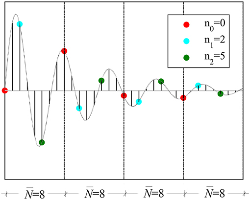
Figure 3. Illustrative example of multi-coset sampling.

Mathematically, the samples of the m-th coset can be written as the output of the filtering operation

$\begin{array}{ll}{y}^m\left[k\right]={{\displaystyle \sum }}_{s=1-\overline{N}}^0{g}_m\left[s\right]x\left[k\overline{N}-s\right]k=0,1,\dots ,P-1& (12)\end{array}$

where P is the total number of the $\overline{N}$-length blocks and the filter coefficients are given as

$\begin{array}{ll}{g}_m\left[s\right]=\{\begin{array}{c}1,s=n_m\\ 0,s\ne n_m\end{array}& (13)\end{array}$

in which s = [1–N, 2–N, …, 0] is arranged in descending order.

Consider, next, an array of D sensors and M cosets as shown in Figure 2. The cross-correlation sequences of response acceleration signals sampled at Nyquist rate, x_i[v], from all i = 1, 2, …, D sensors are theoretically defined as

$\begin{array}{ll}{r}_{x_i{x}_j}\left[\ell \right]={\text{E}}_x\left\{x_i\left[v\right]x_j\left[v-\ell \right]\right\}i,j=1,2,\dots ,D;\ell \in \mathbb{Z}& (14)\end{array}$

where E is the mathematical expectation operator. It is herein assumed that the sequences in Equation (14) take on negligible values outside the range −L ≤ ℓ ≤ L. Further, the cross-correlation sequences of the compressed measurements $y_i^m\left[k\right]$ from all m = 0, 1, …, $\overline{M}-1$ cosets and i = 1, 2, …, D sensors, are written as

$\begin{array}{l}\hfill r_{y_i^a,y_j^b}\left[\ell \right]=\text{E}\left\{y_i^a\left[k\right]y_j^b\left[k-\ell \right]\right\}\\ \hfill i,j=1,2,\dots ,D;a,b=0,1,\dots ,\overline{M}-1;-L\le \ell \le L& (15)\end{array}$

It can be shown (Gkoktsi and Giaralis, 2019) that the sequences in Equations (14) and (15) are related by the following key equation

$\begin{array}{ll}{\text{r}}_{y_i{y}_j}={\text{R}}_g{\text{r}}_{x_i{x}_j}& (16)\end{array}$

where ${\text{r}}_{x_i{x}_j}\in {ℝ}^{\overline{N}(2L+1)\times D}$ is a matrix collecting all cross-correlation sequences of response acceleration signals r_xixj[ℓ], ${\text{r}}_{y_i{y}_j}\in ℝ{}^{{\overline{M}}^2(2L+1)\times D}$ is a matrix collecting all cross-correlation sequences of the compressed measurements $r_{y_i^a,y_j^b}\left[\ell \right]$, and ${\text{R}}_g\in {ℝ}^{{\overline{M}}^2(2L+1)\times \overline{N}(2L+1)}$ is a sparse pattern correlation matrix populated by the multi-coset sampling pattern cross-correlations

$\begin{array}{ll}{r}_{g_a,g_b}\left[\tau \right]={{\displaystyle \sum }}_{s=1-\overline{N}}^0{g}_a\left[s\right]g_b\left[s-\tau \right]=\delta \left[\tau -(n_a-n_b)\right]& (17)\end{array}$

where δ[u] = 1 for u = 0 and δ[u] = 0 for u ≠ 0. Note that Equation (16) defines an overdetermined system of linear equations which can be solved for r_xixj without any sparsity assumptions, provided that R_c is full column rank. The latter is satisfied for M² ≥ N (Ariananda and Leus, 2012).

From the practical/computational viewpoint, the unbiased estimator

$\begin{array}{ll}{\widehat{r}}_{y_i^a,y_j^b}\left[\ell \right]=\frac{1}{P-\left|\ell \right|}{\displaystyle \sum _{l=\text{max}\left\{0,\ell \right\}}^{P-1+\text{min}\left\{0,\ell \right\}}}{y}_i^a\left[l\right]y_j^b\left[l-\ell \right]& (18)\end{array}$

can be readily employed to approximate the sequences in Equation (15) using all compressed measurements wirelessly transmitted to a central unit (server) from all D sensors as indicated in Figure 2. These estimates are collected in the matrix ${\widehat{r}}_{y_i{y}_j}\in ℝ{}^{{\overline{M}}^2(2L+1)\times D}$. Next, an estimate of the response acceleration PSD matrix at discrete frequencies with frequency discretization step (resolution)

$\begin{array}{ll}\Delta \omega =\frac{2\pi }{(2L+1)\overline{N}}& (19)\end{array}$

is computed at the server through the formula (Gkoktsi et al., 2015; Gkoktsi and Giaralis, 2019)

$\begin{array}{ll}{\widehat{G}}_{x_i{x}_j}={\text{F}}_{(2L+1)\overline{\text{N}}}{\left({\text{R}}_g^{\text{T}}{\overline{W}}^{-1}{\text{R}}_g\right)}^{-1}{R}_g^{\text{T}}{\overline{W}}^{-1}{\widehat{\text{r}}}_{y_i{y}_j},& (20)\end{array}$

where ${\text{F}}_{(2L+1)\overline{N}}\in {ℂ}^{\overline{N}(2L+1)\times \overline{N}(2L+1)}$ is the standard DFT matrix. In the last equation, $\overline{\text{W}}$ is a weighting matrix, and the superscript “−1” denotes matrix inversion. Ultimately, in stage III, the PSD matrix in Equation is treated by the standard FDD algorithm to estimate R structural mode shapes, ${\widehat{\varphi }}_r$, and natural frequencies, f_r, r = 1, 2, …, R.

The critical parameters of the herein briefly reviewed PSBS approach regulating CR are the number of cosets, $\overline{M}$, and the length$\overline{N}$of the blocks in Figure 3, subject to the two constraints $\overline{M}<\overline{N}$and ${\overline{M}}^2\ge \overline{N}$. Once the values of $\overline{M}$ and $\overline{N}$ are fixed, the weighting matrix $\overline{\text{W}}$ in Equation and the sampling pattern n is determined by solving a constrained least-squares optimization problem as detailed in Tausiesakul and González-Prelcic (2013) relying on the criterion ${\widehat{\text{r}}}_{x_i{x}_j}=arg{min}_{{\text{r}}_{x_i{x}_j}}\Vert {\widehat{\text{r}}}_{y_i{y}_j}-{\text{R}}_g{\text{r}}_{x_i{x}_j}{\Vert }_{\overline{\text{W}}}^2$, where $\Vert \text{a}{\Vert }_{\overline{\text{W}}}^2={\text{a}}^{\text{T}}\overline{\text{W}}\text{a}$ is the weighted version of the Euclidean norm.

Assessment for Signal Recovery in Time and in Frequency Domain

The effectiveness and applicability of both considered approaches for vibration-based modal identification relies on the accuracy of their respective information recovery operations from compressed measurements. That is, time-domain signal reconstruction/recovery in the STCS-rwPBDN approach, and frequency domain PSD estimation/recovery in the PSBS-based approach. In this section, the performance of the above recovery operations is numerically assessed using field-recorded response acceleration data from an operational Wind Turbine (WT) in Lübbenau, Germany (Klis and Chatzi, 2016a). The considered structure was instrumented with wired high-accuracy MEMs accelerometer sensors located at the cross-section of the WT tower at 80 and 100 m height. The instrumentation layout of the WT is shown in Figure 4. Acceleration data were conventionally acquired at a uniform-in-time sampling rate of 200 Hz measured for ~10 min every half an hour over a period of 29 days. For the purposes of this work, a small, arbitrarily chosen, sub-set of the recorded acceleration signals is compressed at different compression levels and processed via STCS-rwPBDN and PSBS approaches. PSD estimates and reconstructed signals in time domain are recovered from the compressed data by application of STCS-rwPBDN and PSBS approaches, respectively, while time-histories and non-compressed PSDs of the as-recorded data serve as a basis of comparison. It is expected that the assessment of PSBS information recovery in frequency domain will be most critical given that the level of signal stationarity of the considered data-set is relatively low while PSBS approach relies, theoretically, on signal stationary assumption.

FIGURE 4

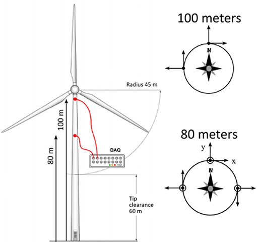
Figure 4. Wind turbine tower and sensor instrumentation set-up (Chatzia and Spiridonakos, 2015).

The numerical assessment of both methods is performed using an acceleration time-series recorded on the 29/12/2013 (at 15:44 p.m.) along the North direction (i.e., y-axis in Figure 4) from the middle sensor in Figure 4 located at 80 m height. The considered acceleration recording was uniformly acquired in time and it consists of N = 172,420 samples. Firstly, baseline adjustment is applied to the raw time-series to remove the mean value and other spurious low-frequency trends. Then, the time-series is band-limited within the frequency range of [0.10, 25.00 Hz] through filtering using a fourth-order Butterworth band-pass filter.

STCS-rwBPDN Approach for Time Domain Signal Recovery

The time-domain reconstruction performance of the STCS-rwBPDN approach is assessed for two compression ratios at CR = {30, 45%}. For a given WT acceleration response, the underlying signal support U is first computed to define the signal's sparsity level, K (i.e., number of components in the spectral domain), as well as the variance of the noisy component, i.e., the complementary set of the support (remaining part of the spectral representation). As elaborated upon in the work of Klis and Chatzi (2016a,b), this is used to prescribe error bounds on the reconstructed signal. For the two considered CRs, the obtained signal reconstruction estimates are illustrated in Figure 5 for an acceleration time-window of 400 samples. Comparing the two panels Figure 5, it becomes evident that the increase in the number of transmitted samples results in narrowing the estimated maximal error bounds. Figure 5 also demonstrates the potential of the STCS-rwBPDN approach, when applied in windows of non-stationary response signals, albeit necessitating higher compression rates than the conventional stationary case. The delivered error bounds allow for attributing some level of confidence on the undertaken signal reconstruction operation, which offers a benefit over the alternative (plain) BPDN approach adopted by O'Connor et al. (2014).

FIGURE 5

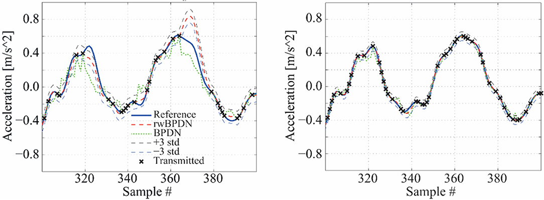
Figure 5. Effect of the increase of transmission level CR on the estimated error bounds: CR = 30% (Left), CR = 45% (Right).

PSBS Approach for Frequency Domain PSD Signal Recovery

The efficacy of the PSBS approach is numerically evaluated herein in terms of recovering quality PSD estimates from computer-simulated compressed acceleration data. These compressed data are derived through the application of the multi-coset sampling pattern [section The Multi-Channel Power Spectrum Blind Sampling (PSBS) Approach] to the corrected (i.e., baseline-adjusted and band-pass filtered), full-length (N = 172,420 samples) acceleration time-series shown in Figure 6A. The Welch periodogram (i.e., conventional PSD estimator) of the full-length time-series before and after band-pass filtering is further plotted in Figure 6B. The two PSDs are normalized to their peak value to facilitate a comparison and have been computed using 4,096 (= 2¹²) points in frequency domain, 8 overlapping segments with 50% overlap, and windowing with a Hanning envelop function. It is observed that peak PSD amplitude occurs at ~1.4 Hz which is the dominant resonant frequency of the monitored WT. Further, it is seen that most important signal information lies in frequencies below 5 Hz, as PSD values above 5 Hz are negligible.

FIGURE 6

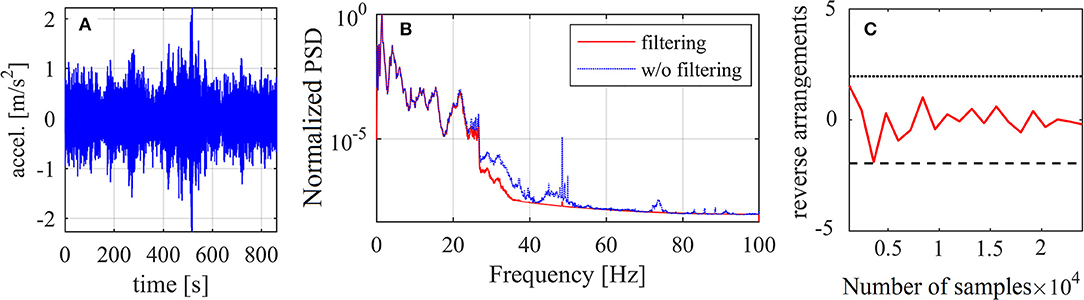
Figure 6. (A) Base-line adjusted and filtered WT response acceleration data-series; (B) normalized Welch periodogram of raw and filtered WT response acceleration data-series in log (db-like) scale; (C) representative reverse arrangement output results for a 2-min long filtered data-series segment.

Given that the PSBS approach anticipates signal stationarity, it is deemed essential to undertake data qualification test to appraise the stationarity level of the recorded time-series considered. To this end, the corrected data Figure 6A is divided in seven time-frames of 2 min duration and the standard non-parametric reverse arrangement method (RAM) is used to test statistically the stationarity hypothesis (Bendat and Piersol, 2010). The outcome of RAM application to a representative 2 min long segment of the considered time-series is presented in Figure 6C demonstrating that the stationarity hypothesis is confirmed within a 95% confidence interval. Positive stationarity hypothesis is confirmed at similar confidence level for the rest of the 2 min-long segments of the data in Figure 6A. Therefore, this WT recorded data can be treated as wide-sense stationary at a high confidence level rendering the application of PSBS meaningful and appropriate.

Next, the WT time-series in Figure 6A is multi-coset sampled at three different CRs, 11, 21, and 31%, using the settings listed in Table 1 and PSBS is applied to the compressed/sub-Nyquist multi-coset samples to obtain single-channel PSD function estimates using the PSD recovery formula in Equation. Specifically, for the case of CR = 31%, the full-length acceleration data-series (N = 172,420 samples) is divided into P = 10,776 ($=N/\overline{N}$) blocks of length $\overline{N}$ = 16 each, and from each block $\overline{M}$ = 5 samples are selected according to the sampling pattern n = [0, 1, 2, 5, 8]. These selected samples are collected in the compressed measurement sequences y^m[k] (m = 0, 1, 2, 3, 4; k = 1, 2, …, P) in Equation resulting in the acquisition and transmission of M = 53,880 compressed samples (i.e., 69% fewer samples compared to the original signal). The estimator ${\widehat{r}}_{y_i^a,y_j^b}\left[\ell \right]$ in Equation is then computed for i = j = 1 (i.e., single-sensor trivial case) and ℓ ∈ [−40, 40] assuming support correlation parameter L = 40. The latter consideration enables PSD function recovery ${\widehat{G}}_{xx}\in {{ℂ}^{1296}}^{\times 1}$ in Equation with frequency discretization step (resolution) Δ ω = 4.85·10⁻³rad/sin Equation. Similar computational steps are taken for the cases of CR = 21 and 11%, based on the relevant parameters in Table 1 which involve the acquisition of 79% (i.e., M = 35,368) and 89% (i.e., M = 18,858) fewer samples compared to the uniformly-sampled full-length signal, respectively.

TABLE 1

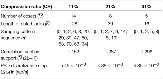
Table 1. Adopted multi-coset sampling and PSBS settings.

Figure 7 plots PSD functions recovered from CR = {11, 31%} (solid red curves) in logarithmic and in linear scale. These functions are normalized to their peak attained value to facilitate comparison against the standard Welch periodogram of the filtered full-length recorded time-series superposed on Figure 7 (dotted blue curves) and normalized in the same manner. It is qualitatively observed that the PSBS-based recovered PSDs lie close to the PSD of the WT data for frequencies up to 5 Hz which take on non-negligible values, and therefore, contain dependable information for modal identification purposes under ambient/operational excitation, for the low CR value (high data compression level). Better quality point-wise matching between the PSBS-based PSDs and the “exact” (non-compressed) PSD of the WT data is achieved even beyond the 0–5 Hz frequency range for the highest CR value considered (i.e., lower data compression level) as expected.

FIGURE 7

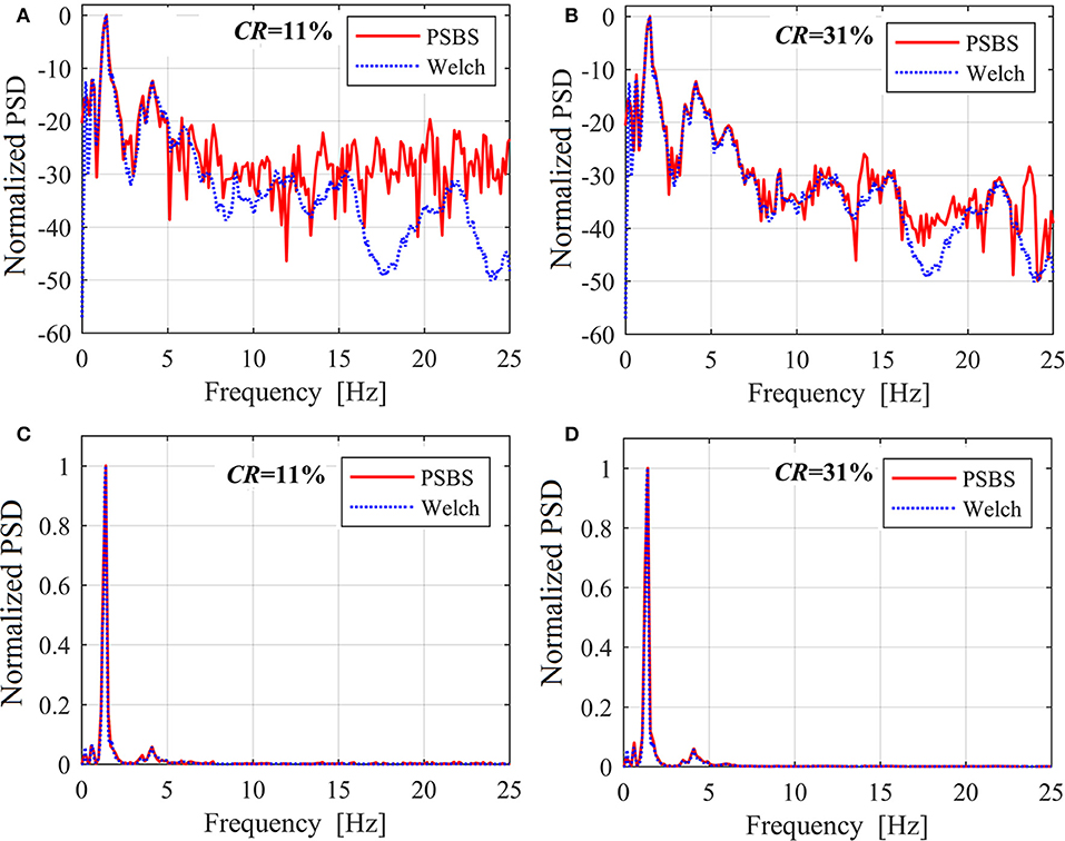
Figure 7. Recovered PSDs using the PSBS approach for different CRs normalized to the peak values: (A) and (B) logarithmic (db-style) scale; (C,D) linear scale.

To discuss further the level of accuracy of the proposed PSBS approach for modal properties identification Table 2 reports the location of the three largest PSD ordinates obtained by simple peak-picking from the recovered functions via PSBS, ${\widehat{f}}_{r,PSBS}$, as well as from the standard Welch periodogram applied to the non-compressed WT acceleration data (CR = 100%), f_{r, Welch}. Further, the percentage difference error

$\begin{array}{ll}\frac{d{f}_r}{f_r}=\frac{|{\widehat{f}}_{r,PSBS}-f_{r,Welch}|}{f_{r,Welch}};r=1,2,3,4& (21)\end{array}$

is also reported as a measure of the quality of the recovered PSDs via the PSBS method. It is seen that the location of the two most prominent PSD peaks (r = 2, 3) is retrieved with <1% error by the PSBS approach for signal compression level as low as 89% below the sampling rate of the original data series. However, the accuracy drops as CR reduces (compression level increases) for the least prominent peak, r = 1, corresponding to an inadequately excited vibration mode whose detection is inherently a challenging task.

TABLE 2

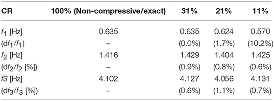
Table 2. Frequency locations of peak PSD ordinates through peak-picking and percentage difference errors for the PSBS approach at various CRs and for Welch periodogram applied on the full-length signal (non-compressed) data-series.

Assessment for Mode Shape Extraction Under Operational Loading Conditions

In this section, the effectiveness of STCS-rwPBDN and PSBS approaches for extracting modes of vibration and natural frequencies is numerically assessed within the OMA context. To this aim, response acceleration time-histories field recorded in a typical highway overpass open to traffic are used. The considered bridge is the Bärenbohlstrasse overpass in Zürich, Switzerland. The structure is 30.90 m long and fairly symmetric along its longitudinal direction. It consists of a solid prestressed-slab with two equal-length spans of 14.75 m each. The deck is supported in all directions at mid-span and in one of the two abutments, while it is only supported in the vertical and transverse directions at the second abutment. The deck was instrumented with a network of 18 conventional wired accelerometers recording vertical acceleration time-histories at 200 Hz sampling rate for ~10 min per hour from 12th July 2013 to 26th July 2014. The layout of the sensor network deployment is shown in Figure 8; more details about the bridge and the monitoring campaign can be found in Klis et al. (2016).

FIGURE 8

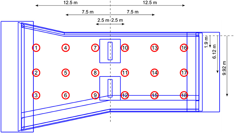
Figure 8. Sensor network layout at the deck of the Bärenbohlstrasse overpass (Klis et al., 2016).

Herein, the first 2 min-long recordings of a dataset of 18 vertical acceleration time-series simultaneously recorded on 19/06/2014 between 15:08:54 and 15:17:51 from each of the 18 sensors of the network are used. The dataset is pre-processed in the same way as the WT data-series case-study in section STCS-rwBPDN Approach for Time Domain Signal Recovery. That is, they are baseline adjusted and band-limited within [0.15, 50 Hz] frequency range using a band-pass 4th-order Butterworth filter. For illustration, Figure 9 plots the band-pass filtered acceleration response signal recorded at sensor #13, together with its magnitude Fourier spectrum. Further, representative results from RAM application to a 1 min long segment of this record is provided demonstrating a very high level of data stationarity (i.e., much higher than the WT data-set; see Figure 6C for comparison).

FIGURE 9

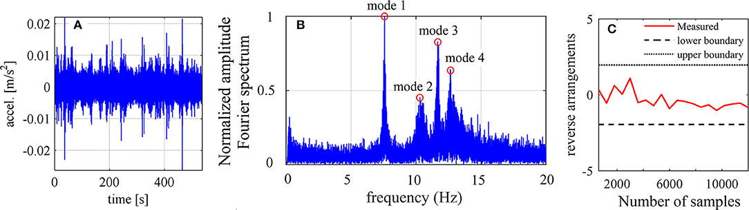
Figure 9. (A) Base-line adjusted and filtered bridge acceleration data-series from sensor #13 in Figure 8; (B) normalized Fourier amplitude spectrum of the data-series in (A); (C) representative reverse arrangement output results for a 2-min long filtered data-series segment.

Next, the first 2 min of the 18 time-series are downsampled at 100 Hz and treated by the STCS-rwPBDN and PSBS approaches. Starting from the STCS-rwPBDN approach, the considered dataset is first partitioned into R = 29 windows (frames) of N_R = 400 samples, and each window is projected into the spectral (Fourier) domain as indicatively shown in Figure 10A for an arbitrarily chosen data-frame of sensor #1 time-series. Following the STCS-rwPBDN methodology in section Spectro-Temporal Compressive Sensing (STCS) Approach via rwBPDN, the spectral (Fourier) coefficients per data frame are then thresholded with a value ϵ_ij = ϵ_l||c_ij||₁/N_R, j = 1…R, which pertains to ϵ_l = 1.5, yielding the spectral domain elements illustrated in Figure 10A. The selected support elements are further used to form a weighting matrix W_ij per data frame. Considering next two different CRs at {36%,11%}, the compressed samples y_i (denoted with a cross in Figure 10B) are selected and used to retrieve the reconstructed time-domain sequence plotted in Figure 10B by a broken line. The standard Natural eXcitation Technique (NeXT) combined with the Eigensystem Realization Algorithm (ERA) are then used to extract estimates of the bridge deck mode shapes, ${\widehat{\varphi }}_r$(r = 1, 2, …), and natural frequencies, ${\widehat{f}}_r$ (r = 1, 2, …), within an OMA context (Brincker and Ventura, 2015).

FIGURE 10

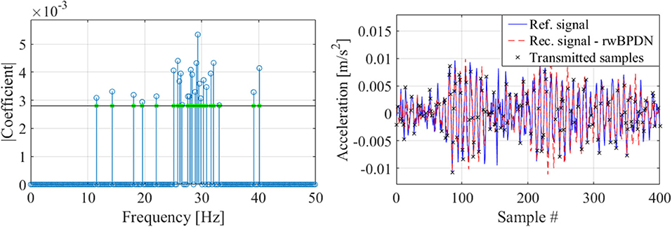
Figure 10. Spectral domain projection (left) and time-domain recovery (right) of data-frame #4, channel #1 at CR = 36%. Crosses indicate transmitted samples used in the recovery process.

Moreover, the same dataset is treated by the PSBS approach using the same procedure and settings as in the WT case-study in Table 1 to recover the PSD matrices ${\widehat{G}}_{x_i{x}_j}\in {ℂ}^{\overline{N}(2L+1)\times 18}$ in Equation for CR = {31, 21, 11%}. The standard FDD algorithm of OMA (Brincker and Ventura, 2015) is applied to these matrices to find estimates of estimates of mode shapes, ${\widehat{\varphi }}_r$(r = 1, 2, …), and natural frequencies, ${\widehat{f}}_r$ (r = 1, 2, …), of the monitored bridge. Indicatively, the first row of panels of Figure 11 plots the first four estimated mode shapes of the bridge for CR = 11% using the PSBS with FDD approach.

FIGURE 11

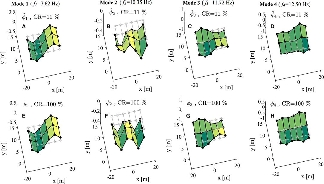
Figure 11. Mode shapes of Bärenbohlstrasse overpass: (A–D): estimated using the PSBS approach for CR = 11%; (E–H): “exact” (non-compressive) by application of FDD to the full-length recorded data.

The quality/accuracy of modal properties extracted through the STCS-rwPBDN and PSBS approaches is assessed by comparison to natural frequencies, f_r (r = 1, 2, …), and mode shapes, ϕ_r (r = 1, 2, …), obtained by application of the standard FDD to the full-length (non-compressive) dataset of recorded acceleration time-histories which are treated as the “exact” ones. The second row of panels of Figure 11 plots the first four exact mode shapes and further reports the corresponding natural frequencies. Table 3 reports percentage difference errors of the first four natural frequencies of the bridge deck obtained through coupling the STCS-rwPBDN with NeXT-ERA as well as the PSBS with FDD for different CRs with respect to the exact (non-compressive) ones as per Equation (21). It further collects the corresponding Modal Assurance Criterion (MAC) values defined by (Brincker and Ventura, 2015)

$\begin{array}{ll}MAC=\frac{{\left|{\varphi }_r^{\text{T}}{\widehat{\varphi }}_r\right|}^2}{\Vert {\varphi }_r{\Vert }_2^2\Vert {\widehat{\varphi }}_r{\Vert }_2^2}r=1,2,3,4& (22)\end{array}$

to quantitatively compare the mode shapes extracted through the two compressive/sub-Nyquist approaches considered for different CRs with the exact mode shapes. As a commonly used criterion, estimated mode shapes with MAC > 0.90 are regarded to be acceptably close to the exact ones.

TABLE 3

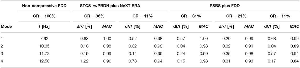
Table 3. Quantitative assessment of the accuracy of natural frequencies and mode shapes for the bridge case-study obtained by the PSBS with FDD and by the STCS-rwPBDN with NeXT-ERA approaches for different CRs vis-à-vis standard non-compressive FDD approach.

By examining the numerical data in Table 3, it is seen that both STCS-rwPBDN and PSBS approaches are quite accurate in identifying natural frequencies as the error df/f is well below 1% even for the lowest CR = 11% value corresponding to average sampling rate of 89% below the Nyquist rate which equals to 100 Hz for the dataset considered. Further, the PSBS approach yields accurate mode shapes across the board for CR as low as 21%. For the lowest CR (= 11%), PSBS is still capable of extracting the 1st and 3rd modes with acceptable accuracy, as can be visually appreciated by comparing the mode shapes in Figures 11A,C with Figures 11E,G, respectively. However, PSBS fails to pass the MAC > 0.90 criterion for 2nd and 4th modes for CR = 11% as highlighted in boldface font in Table 3 (compare also Figures 11B,D with Figures 11F,H). This is readily attributed to the fact that 2nd and 4th modes are significantly less excited than 1st and 3rd modes as evidenced by the amplitude of the respective Fourier coefficients in Figure 9B. Higher than 11% CR (i.e., larger number of measurements) is required for the PSBS approach to accurately probe into the least excited 2nd and 4th modes. On the antipode, the STCS-rwPBDN approach provides good estimates for all four modes even at CR = 11%.

To highlight the practical merit of considering reduced CR values, estimates of daily energy consumption and battery lifetime savings for a single wireless sensor node of the WSN in Figure 8 are further reported in Table 4. The data account for only data transmission power requirement as this is by far the most energy demanding sensor operation (e.g., Lynch, 2007). The reported estimates are based on the assumption that each sensor acquires 2 min long acceleration signals at Nyquist rate (CR = 100%) with Fs = 100 Hz (Ts = 0.01 s) under operational conditions every 1 h (i.e., a dataset of Q = 24 signals are collected daily per sensor with each signal comprising 12,000 measurements for CR = 100%). Power consumption during transmission of P_t = 103.8 mW is taken based on the specification of a typical wireless sensor used for SHM: the WiseNode v4 developed by Novakovic et al. (2009). Table 4 reports transmission time, energy consumption, and battery lifetime for three different CRs previously considered in Table 3. For illustration, computations pertaining to the case of CR = 11% are presented in detail for which only 12,000 × 0.11 = 1,320 compressed measurements per hour are wirelessly transmitted. Assuming that ADC units with 16 bits (i.e., 2 bytes) resolution are used, I_FWD = 2,640 bytes of data package information are generated per compressed sequence taking t = (I_FWD/I_t1) × t₁ = 7.54 s to be wirelessly transmitted to the server, where I_t1 = 7 bytes is the information carried within one data package and t₁ = 0.02 s is the time required for package transmission (Novakovic et al., 2009). Thus, t_tot = Q × 7.54 = 181 s (or 0.05 h) are required for the daily transmission of all compressed acceleration response data, consuming E_tot = P_t × t_tot = 18.79 J of energy per day. It is further assumed that sensor energy supply of 3 V comes from two AA-sized batteries with nominal voltage V_n = 1.5 V and capacity C_n = 3,000 mAh, providing energy E_b = 64,800 J. A continuous discharge current is taken to occur in the batteries resulting in ξ = 1% annual energy loss. Then, sensor battery lifetime, given by

$\begin{array}{ll}{\text{T}}_b=\frac{E_b}{E_{tot}+E_b\times \xi /365},& (23)\end{array}$

is estimated as T_b = 104.8 months.

TABLE 4

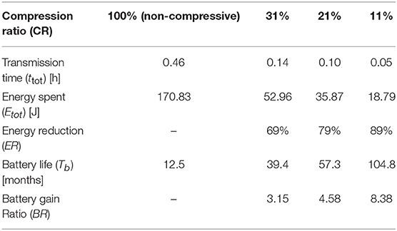
Table 4. Daily sensor energy consumption and battery lifetime gains due to wireless data transmission for various CRs.

Similar calculations are performed to estimate E_tot and T_b for CR = 21, 31% as well as CR = 100% (non-compressive transmission) shown in Table 4. The latter case is the one most widely considered in the literature in comparative studies on energy savings quantification in wireless sensors (e.g., O'Connor et al., 2013, 2014; Klis and Chatzi, 2016b). In this respect, Table 4 reports energy reduction and battery gain ratio for all CR <100% examined with respect to CR = 100% given as

$\begin{array}{lll}\hfill \text{ER}& =& \frac{{E_{tot}|}_{CR=100}-{E_{tot}|}_{CR}}{{E_{tot}|}_{CR=100}}\times \text{100}\%\text{ and}\\ \hfill {\text{T}}_b& =& \frac{{T_b|}_{CR}}{{T_b|}_{CR=100}},& (24)\end{array}$

respectively. Evidently, battery life expectancy increases dramatically as CR reduces: it more than triples for CR = 31% compared to non-compressive sampling/transmission, while it increases more than 8 times for CR = 11%. In this respect, through collective consideration of the data in Tables 3, 4, it can be concluded that the considered approaches effectively support more sustainable wireless monitoring systems having reduced maintenance costs and environmental impact associated with sensors battery replacement which can be scheduled at much longer intervals without significant deterioration to the accuracy of the estimated modal properties compared to Nyquist data sampling.

Note, however, that in a practical setting, the choice of CR (and corresponding battery lifetime gains) is normally dictated by the sought level of accuracy in extracting modal properties according to the monitoring purpose and objectives. If accurate modal properties estimation in the absolute sense is desired (e.g., for updating computational models of as-built structures, or for designing/assessing the performance of vibration control devices, such as tuned mass dampers, to reduce dynamic response of structures) higher CR values should be adopted (e.g., CR > 31%). In such cases, battery lifetime gains may be relatively low but, at the same time, these gains may be a less important practical consideration. On the antipode, lower CR values (e.g., CR = 21% or lower) may be adopted in monitoring campaigns for which extending sensor battery lifetime becomes a priority over modal extraction accuracy. One such example is in long-term/permanent structural monitoring deployments aiming to detect structural damage (e.g., due to natural deterioration or after an extreme event), in which case reducing battery replacement frequency, and thus maintenance costs, becomes important and may be a main criterion for installing a monitoring system in the first place (e.g., O'Connor et al., 2014), while accuracy of modal properties in the absolute sense is less important since changes to modal properties (as a function of environmental conditions) are of interest.

In every case, the data furnished in Tables 3, 4 are only indicative and should be used/interpreted comparatively rather than in an absolute. Indeed, recorded measurements considered to derive modal properties have been obtained by a wired sensor network and, therefore, do not account for the influence of errors that may be encountered in WSNs, such as loss of synchronization. Moreover, power consumption (and thus battery lifetime gains) varies from sensor to sensor in a WSN and is dependent on several factors including environmental conditions, distance from sensors to base station, data communication protocols, etc. In this regard, field deployment of WSNs operating on PSBS and STCS-rwPBDN is required to appraise the quality of modal properties and battery gains in an absolute application-specific sense; such consideration falls outside the scope of this work.

Concluding Remarks

The applicability and performance of two recently proposed approaches for output-only modal identification supporting low energy consumption wireless sensors has been comparatively demonstrated through numerical assessment using field recorded acceleration data. Both the approaches aim to reduce wireless data transmission payloads by considering compressed structural acceleration responses acquired non-uniformly in time at sub-Nyquist average sampling rates. The first, STCS-rwBPDN, approach aims to recover acceleration time-histories in time-domain from low-rate randomly acquired measurements using the rwBPDN algorithm of compressing sensing. The accuracy and efficiency of this operation requires knowledge of the signal support in the frequency domain prior to transmission of compressed measurements from sensor nodes to a central server where time-domain reconstruction takes place. This knowledge is gained through sampling and interrogation of full-length acceleration data at the sensing nodes as well as sensors/server exchange of pertinent information. In this regard, STCS-rwBPDN can recover the time trace of response acceleration signals in a deterministic setting and, therefore, can be coupled at the post-processing back-end with any standard OMA technique for modal properties extraction. Nevertheless, this flexibility comes at the cost of a relatively sophisticated wireless data communication strategy as well the necessity to sample signals at Nyquist frequency or above at sensors front-end. The second, PSBS, approach is effectively a spectral estimation technique aiming to recover second-order statistics (i.e., correlation or PSD functions) of response acceleration signals treated as stationary random processes and acquired through low-rate deterministic non-uniform-in-time multi-coset sampling. Compared to STCS-rwBPDN, the main practical advantage of the PSBS-based approach is its simplicity of wireless communication within WSNs as well as minimal on-sensor data interrogation. Low-rate multi-coset samples can be acquired using some pre-specified sampling pattern at each sensor and communicated as-recorded directly to a server. This high level of data transmission simplicity is made possible by the inherent signal agnostic attribute of PSBS which does not require any prior knowledge about signal spectral support. However, PSBS approach cannot retrieve time traces of the acquired signals and this limits the system identification methodologies that can be applied at the back end of the approach to those relying on only second-order signal statistics for modal properties extraction. One such method is the FDD which was herein coupled with PSBS to deliver mode shapes and natural frequencies directly from the low-rate multi-coset sampled response accelerations.

The validation of the two approaches was carried out by considering field-recorded acceleration data obtained from conventional wired sensor deployments in an operating on-shore wind turbine and in a highway overpass (bridge) open to traffic. The recorded data have been compressed to different levels (CRs) and processed by both approaches. PSBS captured successfully salient frequency domain information for the dataset of the wind turbine for CR as low as 11% (i.e., using 89% less measurements from the conventionally sampled dataset). This demonstrates the potential of the method to treat real-life data that may deviate from perfect stationary signal conditions. Similarly, STCS-rwBPDN was shown to recover faithfully time traces of the wind turbine data set at same low CR levels (11%). In view of these results, it is concluded that both methods are equally promising for SHM of wind turbines using low-rate acceleration measurements. Moreover, STCS-rwBPDN coupled with standard NeXT-ERA was able to retrieve quality estimates of mode shapes and natural frequencies of the bridge case-study again at CR = 11%. PSBS was also able to capture with high accuracy the same mode shapes for CR = 21% while only the two most significant ones were retrieved at CR = 11% satisfactorily.

In view of the herein reported numerical results, it is concluded that both the considered approaches are capable for accurate output-only system identification of large-scale civil infrastructure while being, to a good extend, complementary. Moreover, it is noted that both approaches can be used to acquire alternative types of signals to acceleration data, such as tilt measurements and dynamic strains considered in SHM. It is thus envisioned that smart sensing nodes may incorporate both these approaches for reducing data transmission payloads in WSNs which will allow operators to switch between the two depending on their monitoring needs at any given time: time-series recovery at, perhaps, some increased data transmission requirements and more intense on-sensor processing or modal properties recovery at minimum wireless data exchange and with minimum on-sensor data interrogation.

Still, note that all datasets considered in this work pertain to wired sensors and, therefore, are free from errors that are more common in WSNs, such as missing data or gaps in data due to data loss in wireless transmission, loss of synchronization among sensors, etc. The extent of such errors and its potential impact to the quality of monitoring (e.g., accuracy of extracted mode shapes and natural frequencies) is application-specific depending on factors, such as the technology and quality of the sensor nodes used, the topology of WSN, the nature and scale of the monitored structure, the environmental conditions etc. Moreover, the same factors influence sensor energy consumption and ultimately battery lifetime. In this regard, consideration of long-term real-life field deployments of WSNs operating on the examined approaches is further warranted to verify the accuracy and battery life prolongation of the approaches for full-fledged monitoring of large-scale civil engineering structures. This consideration is left for future work.

Data Availability

The datasets generated for this study are available on request to the corresponding author.

Author Contributions

AG and EC conceived the study. KG performed all data processing related to the PSBS approach. RK and VD performed all data processing related to the STCS approach. KG produced a first draft of the article which was finalized by critical input by AG and EC on introduction, results interpretation, and concluding remarks.

Funding

KG acknowledges the partial financial support received through a Ph.D. studentship by City, University of London. EC would further like to acknowledge support of the ALbert Lück Foundation and the ERC Starting Grant WINDMIL (#679843) on the topic of Smart Monitoring, Inspection and Life-Cycle Assessment of Wind Turbines.

Conflict of Interest Statement

KG is currently employed by AKT-II.

The remaining authors declare that the research was conducted in the absence of any commercial or financial relationships that could be construed as a potential conflict of interest.

Acknowledgments

Sections The Multi-Channel Power Spectrum Blind Sampling (PSBS) Approach, STCS-rwBPDN Approach for Time Domain Signal Recovery, and part of section Assessment for Mode Shape Extraction Under Operational Loading Conditions of this paper form part of the Ph.D. thesis of KG (Gkoktsi, 2018) supervised by AG.

References

Ariananda, D. D., and Leus, G. (2012). Compressive wideband power spectrum estimation. IEEE Trans. Signal Proc. 60, 4775–89. doi: 10.1109/TSP.2012.2201153

CrossRef Full Text | Google Scholar

Avendaño-Valencia, L. D., Chatzi, E. N., Koo, K. Y., and Brownjohn, J. M. W. (2017). Gaussian process time-series models for structures under operational variability. Front. Built Environ. 3:69. doi: 10.3389/fbuil.2017.00069

CrossRef Full Text | Google Scholar

Bao, Y., Beck, J. L., and Li, H. (2010). Compressive sampling for accelerometer signals in structural health monitoring. Struct. Health Monitor. 10, 235–246. doi: 10.1177/1475921710373287

CrossRef Full Text | Google Scholar

Becker, S., Bobin, J., and Candès, E. J. (2011). NESTA: a fast and accurate first-order method for sparse recovery. SIAM J. Imaging Sci. 4, 1–39. doi: 10.1137/090756855

CrossRef Full Text | Google Scholar

Bendat, J. S., and Piersol, A. G. (2010). Random Data: Analysis and Measurement Procedures. 4th Edn. Hoboken, NJ: John Wiley & Sons Inc.

Google Scholar

Brincker, R., and Ventura, C. E. (2015). Introduction to Operational Modal Analysis. Hoboken, NJ: John Wiley & Sons Inc.

Google Scholar

Candès, E. J., and Plan, Y. (2011). A probabilistic and RIPless theory of compressed sensing. IEEE Trans. Inform. Theory 57, 7235–7254. doi: 10.1109/TIT.2011.2161794

CrossRef Full Text | Google Scholar

Candès, E. J., and Romberg, J. (2007). Sparsity and incoherence in compressive sampling. Inv. Probl. 23, 969–985. doi: 10.1088/0266-5611/23/3/008

CrossRef Full Text | Google Scholar

Candès, E. J., Romberg, J., and Tao, T. (2006). Robust uncertainty principles: exact signal reconstruction from highly incomplete frequency information. IEEE Trans. Inform. Theory 52, 489–509. doi: 10.1109/TIT.2005.862083

CrossRef Full Text | Google Scholar

Candès, E. J., and Tao, T. (2006). Near-optimal signal recovery from random projections; universal encoding strategies? IEEE Trans. Inform. Theory 52, 5406–5425. doi: 10.1109/TIT.2006.885507.

CrossRef Full Text | Google Scholar

Chatzia, E. N., and Spiridonakos, M. D. (2015). “Structural identification and monitoring based on uncertain/limited information,” in EVACES'15, 6th International Conference on Experimental Vibration Analysis for Civil Engineering Structures (Dbendorf). doi: 10.1051/matecconf/20152401003

CrossRef Full Text | Google Scholar

Donoho, D. L. (2006). Compressed sensing. IEEE Trans. Inform. Theory 52, 1289–1306. doi: 10.1109/TIT.2006.871582

CrossRef Full Text | Google Scholar

Eslani, N., Aghagolzadeh, A., and Andargoli, S. M. H. (2014). “Recovery of compressive video sensing via dictionary learning and forward prediction,” in 7th International Symposium on Telecommunications (Tehran). doi: 10.1109/ISTEL.2014.7000819

CrossRef Full Text

Farrar, C. R., and Worden, K. (2012). Structural Health Monitoring: A Machine Learning Perspective. Hoboken, NJ: John Wiley & Sons Inc.

Google Scholar

Fuentes, R., Mineo, C., Pierce, S. G., Worden, K., and Cross, E. J. (2019). A probabilistic compressive sensing framework with applications to ultrasound signal processing. Mech. Syst. Signal Process. 117, 383–402. doi: 10.1016/j.ymssp.2018.07.036.

CrossRef Full Text | Google Scholar

Gkoktsi, K. (2018). Compressive techniques for sub-Nyquist data acquisition & processing in vibration-based structural health monitoring of engineering structures (PhD Thesis). University of London, London.

Google Scholar

Gkoktsi, K., and Giaralis, A. (2017). Assessment of sub-Nyquist deterministic and random data sampling techniques for operational modal analysis. Struct. Health Monitor. 16, 630–646. doi: 10.1177/1475921717725029

CrossRef Full Text | Google Scholar

Gkoktsi, K., and Giaralis, A. (2019). A multi-sensor sub-Nyquist power spectrum blind sampling approach for low-power wireless sensors in operational modal analysis applications. Mech. Syst. Signal Process. 116, 879–899. doi: 10.1016/j.ymssp.2018.06.049

CrossRef Full Text | Google Scholar

Gkoktsi, K., Giaralis, A., and TauSiesakul, B. (2016). “Sub-Nyquist signal-reconstruction-free operational modal analysis and damage detection in the presence of noise,” in Proceedings of SPIE on Sensors and Smart Structures Technologies for Civil, Mechanical, and Aerospace Systems, 9803. doi: 10.1117/12.2219194

CrossRef Full Text | Google Scholar

Gkoktsi, K., Tausiesakul, B., and Giaralis, A. (2015). “Multi-channel sub-Nyquist cross-spectral estimation for modal analysis of vibrating structures,” in Proceedings of the 22nd International Conference on Systems, Signals and Image Processing, 287–290.

Google Scholar

Klis, R., and Chatzi, E. N. (2016a). Data recovery via hybrid sensor networks for vibration monitoring of civil structures. Int. J. Sust. Mater. Struct. Syst. 2, 161–184. doi: 10.1504/IJSMSS.2015.078373

CrossRef Full Text | Google Scholar

Klis, R., and Chatzi, E. N. (2016b). Vibration monitoring via spectro-temporal compressive sensing for wireless sensor networks. Struct. Infrastr. Eng. 13, 195–209. doi: 10.1080/15732479.2016.1198395

CrossRef Full Text | Google Scholar

Klis, R., Chatzi, E. N., and Spiridonakos, M. (2016). “Validation of vibration monitoring via spectro-temporal compressive sensing for wireless sensors networks using bridge deployment data,” in Proceedings of the 8th International Conference on Bridge Maintenance, Safety and Management (IABMAS 2016).

Limongelli, M. P., Chatzi, E. N., Döhler, M., Lombaert, G., and Reynders, E. (2016). Towards extraction of vibration-based damage indicators,” in EWSHM-8th European Workshop on Structural Health Monitoring (Bilbao).

Google Scholar

Lynch, J. P. (2007). An overview of wireless structural health monitoring for civil structures. Philosoph. Trans. R. Soc. A365, 345–372. doi: 10.1098/rsta.2006.1932

CrossRef Full Text | Google Scholar

Nagayama, T., Spencer, B. F. Jr, and Jennifer, A. Rice. (2009). Autonomous decentralized structural health monitoring using smart sensors. Struct. Control Health Monitor. 16, 842–859. doi: 10.1002/stc.352

CrossRef Full Text | Google Scholar

Nesterov, Y. (2005). Smooth minimization of non-smooth functions. Math. Programm. 103, 127–152. doi: 10.1007/s10107-004-0552-5

CrossRef Full Text | Google Scholar

Novakovic, A., Meyer, J., Bischoff, R., Feltrin, G., Motavalli, M., El-Hoiydi, A., et al. (2009). Low Power Wireless Sensor Network for Monitoring Civil Infrastructure. Technical Report, Empa, Swiss Federal Laboratories for Materials Testing and Research. CSEM, Swiss Center for Electronics and Microtechnology.

O'Connor, S. M., Lynch, J. P., and Gilbert, A. C. (2013). Implementation of a Compressive Sampling Scheme for Wireless Sensors to Achieve Energy Efficiency in a Structural Health Monitoring System,” in SPIE Smart Structures and Materials + Nondestructive Evaluation and Health Monitoring SPIE, 11.

Google Scholar

O'Connor, S. M., Lynch, J. P., and Gilbert, A. C. (2014). Compressed sensing embedded in an operational wireless sensor network to achieve energy efficiency in long-term monitoring applications. Smart Mater. Struct. 23:085014. doi: 10.1088/0964-1726/23/8/085014

CrossRef Full Text | Google Scholar

Park, J. Y., Wakin, M. B., and Gilbert, A. C. (2014). Modal analysis with compressive measurements. IEEE Trans. Signal Process. 62, 1655–1670. doi: 10.1109/TSP.2014.2302736

CrossRef Full Text | Google Scholar

Razaviyayn, M., Tseng, H.-W., and Luo, Z.-Q. (2014). “Dictionary learning for sparse representation: complexity and algorithms,” Proceedings-ICASSP, IEEE International Conference on Acoustics, Speech and Signal Processing (Florence). doi: 10.1109/ICASSP.2014.6854604

CrossRef Full Text | Google Scholar

Reynders, E., Gersom, W., and De Roeck, G. (2013). Output-only structural health monitoring in changing environmental conditions by means of nonlinear system identification. Struct. Health Monitor. 13, 82–93. doi: 10.1177/1475921713502836

CrossRef Full Text | Google Scholar

Shi, H., Worden, K., and Cross, E. J. (2016). A non-linear cointegration approach with applications to structural health monitoring. J. Phys. 744:012025. doi: 10.1088/1742-6596/744/1/012025

CrossRef Full Text | Google Scholar

Straub, D., Eleni, C., Elizabeth, B., Wim, C., Döhler, M., Faber, M. H., et al. (2017). “Value of information: a roadmap to quantifying the benefit of structural health monitoring,” in ICOSSAR-12th International Conference on Structural Safety & Reliability (Vienna).

Google Scholar

Tausiesakul, B., and González-Prelcic, N. (2013). “Power spectrum blind sampling using minimum mean square error and weighted least squares,” in 2013 Asilomar Conference on Signals, Systems and Computers (Pacific Grove, CA), 153–157.

Google Scholar

Vaswani, N., and Zhan, J. (2016). Recursive recovery of sparse signal sequences from compressive measurements: a review. IEEE Trans. Signal Proc. 64, 3523–3549. doi: 10.1109/TSP.2016.2539138

CrossRef Full Text | Google Scholar

Venkataramani, R., and Bresler, Y. (2001). Optimal sub-Nyquist nonuniform sampling and reconstruction for multiband signals. IEEE Trans. Signal Process. 49, 2301–2313. doi: 10.1109/78.950786

CrossRef Full Text | Google Scholar

Wang, W., Wang, P., Zhou, W., and Li, H. (2015). “The study of damage identification based on compressive sampling,” in Proceedings SPIE 9437, Structural Health Monitoring and Inspection of Advanced Materials, Aerospace, and Civil Infrastructure 2015, 94371L. doi: 10.1117/12.2084061

CrossRef Full Text | Google Scholar

Wang, Y., and Hong, H. (2015). Damage identification scheme based on compressive sensing. J. Comp. Civil Eng. 29:04014037. doi: 10.1061/(ASCE)CP.1943-5487.0000324

CrossRef Full Text | Google Scholar

Yang, Y., and Nagarajaiah, S. (2015). Output-only modal identification by compressed sensing: non-uniform low-rate random sampling. Mech. Syst. Signal Process. 56–57, 15–34. doi: 10.1016/j.ymssp.2014.10.015

CrossRef Full Text | Google Scholar

Zou, Z., Bao, Y., Li, H., and Spencer, B. F. (2015). Embedding compressive sensing-based data loss recovery algorithm into wireless smart sensors for structural health monitoring. IEEE Sens. J. 15, 797–808. doi: 10.1109/JSEN.2014.2353032

CrossRef Full Text | Google Scholar