Critical Evaluation of Metaheuristic Algorithms for Weight Minimization of Truss Structures

Introduction

Structural optimization has always been a topic of interest for both the research community and the practicing engineers. It is commonly acknowledged that many real-life problems, featuring a large number of design variables, as well as non-linear objective function(s) and constraints, are quite demanding due to characteristics such as high dimensionality, multimodality, and non-convex feasible regions. In order to address this, researchers were led to Mathematical Programming (MP) and Optimality Criteria (OC) methods (Feury and Geradin, 1978). In MP, the optimization problem is decomposed into simpler subproblems producing designs of good quality which, however, are not necessarily optimal. In OC methods, simple recursion formulas are derived based on assumptions on the optimum design. These formulas may be simple and practical, but often do not converge for highly redundant structures (Feury and Geradin, 1978). Moreover, they do not address the problem properly, in mathematical terms. Interestingly, analytical global sizing optimization of trusses is actually feasible, based on the Cylindrical Algebraic Decomposition algorithm, as shown recently in Charalampakis and Chatzigiannelis (2018).

In contemporary optimization research, metaheuristics, i.e., stochastic algorithms inspired by principles of evolution, swarm intelligence, or other physical phenomena, enriched with simple probabilistic and/or statistical methods, have been established as a prominent tool for solving complex problems. These algorithms possess certain important advantages, such as easy implementation and good performance without being dependent on the gradient or other problem-specific information (Eiben and Smith, 2003). As a result, many applications of metaheuristics in the size optimization of trusses, in particular, have been presented in the literature.

Arguably, the most widely used member of the metaheuristic family is Genetic Algorithms (GAs), which originate from the work of Holland (1975). In GAs, a population of individuals is evolved using appropriate mutation, crossover, and selection operators. Based on Darwin's principles of natural selection and survival of the fittest, promising genetic information is propagated into future generations providing solutions to the optimization problem. Application of GAs to truss size optimization can be found in Koumousis and Georgiou (1994), Rajan (1995), and Coello and Christiansen (2000).

Another popular method of optimization is Simulated Annealing (SA). It is inspired by the annealing process of physical systems which, being at a high-energy state, are gradually cooled down to their minimum energy level. This process was first formulated into an optimization algorithm by Kirkpatrick et al. (1983). An application of SA for size optimization of trusses can be found in Lamberti (2008).

More recently, Geem et al. (2001) proposed Harmony Search (HS) for solving combinatorial optimization problems. HS was inspired by the harmony sought by music players as they improvise the pitches of their instruments. This algorithm has also been used for size optimization of trusses (Lee and Geem, 2004; Lamberti and Pappalettere, 2009; Degertekin, 2012).

In the category of Swarm Intelligence algorithms, Karaboga and Basturk (2008) proposed the Artificial Bee Colony (ABC) algorithm, a stochastic algorithm inspired by the foraging behavior of honey bees. An application of ABC for the size optimization of trusses can be found in Sonmez (2011).

In the same category, Particle Swarm Optimization (PSO) is based on the social sharing of information among members, which produces behavioral patterns that offer an evolutionary advantage (i.e., avoid predators, seek food, and mates). The method, introduced by Kennedy and Eberhart (1995), searches the design space by adjusting the velocities of moving “particles.” As they move, the particles are stochastically attracted toward both their personal best position and the best position found by the whole “swarm” (Clerc and Kennedy, 2002). Many applications of PSO for the size optimization of trusses can be found in the literature (Ray and Saini, 2001; Fourie and Groenwold, 2002; Schutte and Groenwold, 2003; Li et al., 2007; Perez and Behdinan, 2007; Dimou and Koumousis, 2009; Talatahari et al., 2013).

Recently, Rao et al. (2011) proposed a method called “teaching-learning-based optimization” (TLBO), inspired by the learning process of students who are influenced by their teachers as well as their fellow students. Several applications of TLBO for the size optimization of trusses can be found in the literature (Degertekin and Hayalioglu, 2013; Camp and Farshchin, 2014; Dede and Ayvaz, 2015).

Further, the literature is abundant with algorithms inspired by physical phenomena. In Big Bang—Big Crunch (BB-BC), proposed by Erol and Eksin (2006), a random and disordered population, produced at the Big Bang phase, is qualitatively averaged to a single position during the Big Crunch phase. Repeating cycles of these phases guide the algorithm toward optimality. Applications of this method for the size optimization of trusses can be found in Camp (2007) and Kaveh and Talatahari (2009b). Other studies on size optimization of trusses utilize Colliding Bodies Optimization algorithm (CBO) (Kaveh and Ghazaan, 2015; Kaveh and Mahdavi, 2015a,b), which is based on an analogy with one or two-dimensional collisions between bodies, Enhanced Bat Algorithm (EBA) (Kaveh and Zakian, 2014), Ray optimization (RO) (Kaveh and Khayatazad, 2013), Charged System Search (CSS) (Kaveh and Talatahari, 2010), etc.

Notably, Differential Evolution (DE), introduced by Storn and Price (1997), is a stochastic optimization method that is not based on any natural paradigm. An initial version of the algorithm, termed “Genetic Annealing,” was first published in a programmer's magazine in 1994 (Price et al., 2005). Several applications of DE for the size optimization of trusses can be found in the literature (Wu and Tseng, 2010; Bureerat and Pholdee, 2016). Other studies on the same topic that are not nature-inspired are the Adaptive Dimensional Search (Hasançebi and Azad, 2015) and the Guided Stochastic Search (Kazemzadeh Azad and Hasançebi, 2015). In the latter, problem-specific information is utilized as the stochastic optimization process is actually guided by the principle of virtual work.

Finally, researchers have attempted to combine the better features of different algorithms by means of hybridization in order to achieve lighter truss designs, as in Hybrid Particle Swarm—Swallow Swarm (HPSSO) (Kaveh et al., 2014a), Hybrid Particle Swarm—Ant Colony Strategy—Harmony Search (HPSACO) (Kaveh and Talatahari, 2009a), and Swarm Intelligence—Chaos Theory in Chaotic Swarming of Particles (CSP) (Kaveh et al., 2014b).

Metaheuristic algorithms are commonly compared based on mathematical functions with clearly defined characteristics, e.g., unimodal/multimodal, basic/expanded/hybrid, separable/non-separable, convex/non-convex. These characteristics cannot be clearly measured when considering truss size optimization. On the other hand, studies on truss size optimization do not focus on the comparison between algorithms. Usually, only the best final design is compared which may have been found using an excessive computational budget or, in certain cases, with constraint violations. Thus, a need for an overall and unbiased comparison is evident. There are certain publications in the literature regarding this topic (e.g., Keane, 1996; Hasançebi et al., 2009). However, the list of examined algorithms is limited, while there is also a need for more detailed statistical analysis. As measure of the complexity, the number of design variables D, as well as the degree of static indeterminacy SI is indicated for each problem. Some preliminary results on the problem have been presented by Charalampakis (2016), which are greatly revised and extended herein.

Motivated by the above, in this work, an unbiased framework for meaningful comparison between different metaheuristic optimization methods is defined. A strict computational budget is predetermined, according to the dimensionality of the problem. Performance is always measured with respect to function evaluations, i.e., truss analyses, instead of generations or optimization steps. All function evaluations are carefully accounted for. A large sample is collected and analyzed for each algorithm and each problem, to ensure valid statistics. To quantify the robustness of an algorithm, in this study the probability that an arbitrary run will provide a solution of a certain quality (i.e., the probability of a “successful” design) is measured. This is very useful in real-life engineering as it provides a meaningful measure of confidence regarding the optimized design of a structure that has not been studied before or cannot be studied thoroughly due to resource limitations. The lightest solutions which do not violate constraints, produced either herein or (to the best of our knowledge) in the literature, are utilized to screen successful from unsuccessful designs. The success rate of each algorithm is not only evaluated at the end but also monitored throughout the analysis, which reveals interesting information regarding the relative convergence rate.

Based on this framework, a critical evaluation of a number of metaheuristic algorithms is presented, including variants of GAs, PSO, ABC, SA, and DE. The comparison is based on several benchmark problems of varying complexity (number of design variables D = 4–200, degree of static indeterminacy SI = 0–50). Most of these problems have been studied by numerous researchers using a large variety of methods; this allows for absolute rather than relative comparison. The differences in performance between the algorithms are shown and explained. In addition, often a slightly better design is produced, as compared to the existing literature.

Problem Statement

The size optimization problem of a truss with D variables can be formally stated as follows.

Minimize the objective function:

$\begin{array}{ll}f(\text{x})=W(\text{x})+P(\text{x})& (1)\end{array}$

which is subject to:

(a) side constraints x_L ≤ x ≤ x_U (note that vector inequalities are applied element-by-element);

(b) additional constraints (depending on the problem) regarding element stress, buckling stress and/or node displacements.

In Equation (1), x = {x₁, x₂, …, x_D} = a vector which contains the areas of the cross-section of each group of elements, x_L and x_U = vectors which define the minimum and maximum areas, respectively, $W(\text{x})={\displaystyle \sum _{i=1}^D}(L_i{x}_i{\rho }_i)=$ structural weight of the truss, L_i and ρ_i = total length and specific weight of the ith group of bars, and P(x) = penalty function, which is a common method to transform the constrained optimization problem into an unconstrained problem.

The penalty function should follow the so-called “minimum penalty rule,” which is not easy to achieve. This rule dictates that the penalty should be kept as small as possible, yet large enough to keep infeasible solutions from being optimal (Coello, 2002). If the penalty is too large and the optimum solution lies at the boundary of the feasible region, the algorithm will be driven back from the boundary, inside the feasible region, in a strong manner. Also, it will be difficult for the algorithm to move from one feasible region to another if there are more than one, unless they lie very close to each other. On the contrary, using a small penalty will lead to a fruitless exploration of the infeasible region, and thus wasted computational effort, because the penalty will be small as compared to the objective value itself. Since, it is expected that many of the problems examined herein will have optimum solutions lying on the boundary between feasible and infeasible regions, these issues are of importance. There are many types of penalty functions which cannot be examined here; for a survey on the state-of-the-art, see Coello (2002). Since, it is very difficult to define a criterion to quantify what is a “small” violation of the constraints, in this study a static penalty rule is used with a small constant term to keep all best solutions strictly within the feasible domain, i.e., no violation at all is accepted. A normalized constraint violation function is defined as follows:

$\begin{array}{ll}{v}_n^j=\frac{v_o^j}{v_a^j}-1,& (2)\end{array}$

where, $v_n^j$ is the normalized violation of the jth optimization constraint (stress, displacement, buckling stress, etc.), $v_o^j$ is the corresponding value computed for a candidate solution, and $v_a^j$ is the allowable constraint limit. The penalty function is of the form:

$\begin{array}{ll}P(\text{x})={\displaystyle \sum _{j=1}^{N_c}}{\delta }^j\left(A{v}_n^j+B\right),& (3)\end{array}$

where, A = 10⁶, B = 10³, N_c = the number of constraints and δ^j = the activation key defined as:

$\begin{array}{ll}{\delta }^j=\{\begin{array}{c}1,v_n^j>0\\ 0,v_n^j\le 0\end{array}.& (4)\end{array}$

The constant B is used to create a step-like rule, which adds a significant penalty for slight violations. This has proved to be particularly effective and ensures that the best solutions found are devoid of any violations.

Metaheuristic Algorithms

Basic Features of the Trade Study

The following assumptions/rules have been used equally for all algorithms:

1) The same configuration was used for each algorithm in all test problems. For well-established methods, internal parameters were set according to literature. For newly established algorithms, the best combination of parameters was found via parametric analysis.

2) The number of structural analyses required in the optimization process was chosen as the best performance indicator to compare algorithms of different nature and configuration.

3) Thirty independent runs with different random seeds were conducted for each test case and each optimization algorithm in order to obtain statistically significant results. The conclusions are supported by t-tests regarding the significance of the differences between algorithms.

4) A robust random number generator of L'Ecuyer with Bays-Durham shuffle and added safeguards (Press et al., 2002) was used. Henceforth, r = random variable with uniform distribution in the interval (0,1), sampled anew each time it is required, and r = corresponding vector.

5) For each test problem, a value-to-reach (VTR) defines the limit between success and failure. The VTR is 1% heavier than the best feasible design obtained in this study or reported in the literature. Hence, “successful” designs lie very close to the optimum region of design space. The final design is usually more fine-tuned when the VTR threshold is reached early in the optimization process.

6) Regarding the computational budget, it obviously needs to be analogous to the problem difficulty which is generally acknowledged that increases non-linearly in D. This rapid growth in difficulty is commonly referred to as “curse of dimensionality” (Bellman, 1957); however, the allocated computing resources cannot follow this pattern. For this reason, in this study a linear function is used, i.e., the computational budget is set to 2500D structural analyses and the best design is achieved strictly within this limit. This budget balances two conflicting aspects: (a) it is high enough to achieve good designs (often better than those reported in the literature); (b) it is not too excessive to conflict with limitations on computing resources.

7) The unit system utilized is the same as in the original statement of the problem, in order to avoid rounding errors during comparisons.

Cross-sectional areas of elements are rounded to three decimal digits before performing structural analysis in double precision without any further rounding. Literature designs including more than three decimal digits are exactly reproduced in this paper; however, the total weight is re-evaluated and may be slightly different from the source value. The inversion of the stiffness matrix is performed using Gauss-Jordan elimination with full pivoting (Press et al., 2002).

Algorithm Description

Standard Genetic Algorithm (SGA)

The pseudocode of the so-called standard genetic algorithm (SGA) is as follows:

1. Random initialization of the population;

2. Fitness calculation;

3. Selection of individuals to form the new population;

4. Crossover and mutation;

5. Repetition of steps (2–5) until some termination condition is satisfied.

The particular implementation of SGA used herein includes jump and creep mutation, as well as elitism. Jump mutation randomly flips a bit in the genotype, while creep mutation randomly increases or decreases a gene in the phenotype by a single step. Elitism directly transfers the better individual(s) from the previous generation to the next, ensuring that the solution quality will not decrease during evolution. The parameters of SGA are set as follows: gene length L_g = depending on the problem so that the step $(x_U^i-x_L^i)/\left(2^{L_g^i}-1\right)\le {10}^{-3}\forall i\in \left\{1,2,\dots ,D\right\}$; population size P = 50; single crossover with probability 0.7; jump mutation with probability 1/P; creep mutation with probability L_c/D/P ($L_c={\displaystyle \sum _{i=1}^D}{L}_g^i=$ chromosome length in bits); tournament selection with 2 individuals; and elitism (with 1 elite individual).

Hybrid Genetic Algorithm (HGA)

The standard GA formulation is hybridized by combining the search space reduction method (SSRM) and a local optimization algorithm to form the Hybrid Genetic Algorithm (HGA). SSRM is a systematic method which gradually reduces the search space. It facilitates the optimization algorithm by focusing on the promising areas which lead to better solutions. The SSRM embedded in HGA was presented in Charalampakis and Koumousis (2008) and later employed in several cases (e.g., Marano et al., 2011). It is based on a statistical analysis of a population of P candidate designs, where each one is assigned a weight w depending on its quality. For minimization problems:

$\begin{array}{ll}{w}_k=\frac{max(f)}{f_k},k\in \left\{1,2,\dots ,P\right\},& (5)\end{array}$

where max (f) = max {f₁, f₂, …, f_P} is the worst objective value in the population, which corresponds to a weight of unity. The weighted mean value of the design variable i is then calculated as:

$\begin{array}{ll}{m}_i=\frac{{\displaystyle \sum _{k=1}^P}(w_k{x}_{ik})}{{\displaystyle \sum _{k=1}^P}(w_k)},i=\left\{1,2,\dots ,D\right\},& (6)\end{array}$

where x_ik is the value of the ith variable of the kth candidate design. The descriptive weighted standard deviation of the design variable i is given as:

$\begin{array}{ll}{s}_i=\sqrt{\frac{{\displaystyle \sum _{k=1}^P}\left(w_k{\left(x_{ik}-m_i\right)}^2\right)}{{\displaystyle \sum _{k=1}^P}(w_k)}}.& (7)\end{array}$

The new trial lower and upper bounds of the design variable i are formed symmetrically around m_i:

$\begin{array}{ll}\begin{array}{c}{\bar{x}}_{L,j}^i=m_i-q{s}_i\\ {\bar{x}}_{U,j}^i=m_i+q{s}_i\end{array},& (8)\end{array}$

where j is an index for SSRM steps and q is a scalar parameter. Finally, the new range of values of the design variable i is the intersection (common part) of the previous range and the trial range:

$\begin{array}{ll}\left[x_{L,j+1}^i,x_{U,j+1}^i\right]=\left[x_{L,j}^i,x_{U,j}^i\right]\cap \left[{\bar{x}}_{L,j}^i,{\bar{x}}_{U,j}^i\right],& (9)\end{array}$

Based on Equation (9), the search space is not allowed to expand. Instead, it is gradually reduced on a variable-by-variable basis, if justified by the statistical analysis. The scalar q controls the aggressiveness of SSRM. Small values may stochastically lead to exclusion of a promising area in subsequent SSRM steps; large values cancel the beneficial effect of SSRM. In this study, q = 3 is set which is a rather conservative choice (Charalampakis and Koumousis, 2008). The chromosomes of the existing population are substituted by their closest counterpart in the new mapping. If a variable falls out of a new bound, it is set equal to it.

Regarding variable discretization, the gene length is set to 10 bits irrespective of the problem at hand. This leads to a relatively small chromosome length, which greatly facilitates the GA. Refining of the solutions is achieved through SSRM, which is triggered automatically. For the test problems considered in this study, this happens every 5,000, 10,000, 20,000, and 50,000 function evaluations when D = {4}, D = {8, 10, 17}, D = {29} and D = {200}, respectively.

A local optimization algorithm, namely the Greedy Descend Hill Climber (GDHC) (Eiben and Smith, 2003), is also embedded in the HGA. The final 5,000 function evaluations of each run are dedicated to GDHC. The best solution found so far becomes seed; this solution is continuously improved by alternating the bits of the chromosome from left to right, keeping the best result as a reference. When a full cycle has been concluded without improvement of the best result, the local optimum has been found and the process is terminated. If the limit of 5,000 function evaluations is reached prior to finding the local optimum, the reference solution becomes final.

Enhanced Particle Swarm Optimization (EPSO)

In the basic PSO algorithm, the population consists of P particles. Each particle is assigned a position and velocity vector, determined at time instant k by x_k and v_k, respectively. The particles are initialized randomly in the box-constrained design space, so that:

$\begin{array}{ll}{\text{x}}_L\le {\text{x}}_0^m\le {\text{x}}_U\forall m\in \left\{1,2,\dots ,P\right\}.& (10)\end{array}$

The initial velocities of the particles are also chosen randomly:

$\begin{array}{ll}-{\text{v}}_0^{max}\le {\text{v}}_0^m\le {\text{v}}_0^{max}\forall m\in \left\{1,2,\dots ,P\right\},& (11)\end{array}$

where ${\text{v}}_0^{max}=\gamma ({\text{x}}_U-{\text{x}}_L)$ and γ = a scalar parameter. The position vector of a particle m at the next time instant k + 1 is given by:

$\begin{array}{ll}{\text{x}}_{k+1}^m={\text{x}}_k^m+{\text{v}}_{k+1}^m.& (12)\end{array}$

Note that the time step Δt between the distinct time instants is taken equal to unity. The velocity vector ${\text{v}}_{k+1}^m$ is given as:

$\begin{array}{ll}{\text{v}}_{k+1}^m=w_k{\text{v}}_k^m+c_1{\text{r}}_1\circ ({\text{p}}_k^m-{\text{x}}_k^m)+c_2{\text{r}}_2\circ ({\text{p}}_k^g-{\text{x}}_k^m),& (13)\end{array}$

where, w_k = inertia factor at time instant k; c₁, c₂ = cognitive and social parameters, respectively; ${\text{p}}_k^m=$ best-ever position vector of particle m up to and including time instant k; ${\text{p}}_k^g=$ best-ever position vector amongst all particles up to and including time instant k; and the ∘ operator indicates element-by-element multiplication. Note that these formulas are compatible with the diverse “classical” version of PSO (Wilke et al., 2007). The side constraints of Equations (10) and (11) are enforced after each time step.

It is known that standard PSO suffers from convergence rate problems, due to the delicate balance between exploration and exploitation that is required. This was clear in the problems considered in this study, so an enhanced variant is used instead. This variant (EPSO) is based on the work by Fourie and Groenwold (2002) and has been successfully applied in a parameter identification problem (Charalampakis and Dimou, 2010, 2015). The differences with respect to the basic PSO algorithm are the following:

∘ If a period of h consecutive steps passes without the best solution found by the whole swarm being improved, then it is postulated that the velocities are large and “overshooting” prevents the algorithm from locating better solutions. Therefore, a reduction is applied to both the inertia factor and the maximum velocity, as follows:

$\begin{array}{ll}\text{If }f({\text{p}}_k^g)=f({\text{p}}_{k-h}^g)\text{ then }\{\begin{array}{c}{w}_{k+1}=a{w}_k\\ {\text{v}}_{k+1}^{max}=\beta {\text{v}}_k^{max}\end{array}\text{ else }\{\begin{array}{c}{w}_{k+1}=w_k\\ {\text{v}}_{k+1}^{max}={\text{v}}_k^{max}\end{array}.& (14)\end{array}$

∘ The craziness operator imposes a random velocity vector to a particle which hence strays from the swarm and examines other regions of the search space. A probability P_cr is used to activate the operator, as follows:

$\begin{array}{ll}\text{If }r<P_{cr}\text{ then randomly assign }{\text{v}}_{k+1}^m\text{ with -}{\text{v}}_{k+1}^{max}\le {\text{v}}_{k+1}^m\le {\text{v}}_{k+1}^{max}.& (15)\end{array}$

∘ The worst individual is moved to the best ever position found by the swarm.

∘ If the velocity ${\text{v}}_k^m$ leads to an improvement of ${\text{p}}_k^g$ then, instead of Equation (12), the so-called “elite velocity” rule is applied for particle m:

$\begin{array}{ll}{\text{x}}_{k+1}^m={\text{p}}_k^g+c_3{\text{r}}_3\circ {\text{v}}_k^m,& (16)\end{array}$

where c₃ = a scalar parameter. Note the difference between the current implementation and the work by Fourie and Groenwold (2002), where a single random variable r₃ is multiplied by the velocity vector ${\text{v}}_k^m$.

In this study, the parameters of EPSO are set as follows: P = 20, c₁ = 0.5, c₂ = 1.6, γ = 0.4, w₀ = 1.40, h = 3, a = 0.99, β = 0.95, P_cr = 0.22, and c₃ = 1.30.

Artificial Bee Colony (ABC)

According to the ABC method, the colony of artificial bees is divided into two equal groups, i.e., the employed bees and the onlookers. Also, the number of food sources (possible solutions) around the hive is equal to the number of employed bees. Initially, the ABC initializes randomly SN/2 food source positions, where SN = total colony size. Next, the food source positions are subjected to repeated cycles of improvement as follows.

The employed bee i modifies the position vector of the associated food source i:

$\begin{array}{ll}{\bar{x}}_{ij}=x_{ij}+(2r-1)(x_{ij}-x_{kj}),& (17)\end{array}$

where i, k ∈ {1, 2, …, SN/2} = random indices with i ≠ k and j ∈ {1, 2, …, D} = a randomly chosen dimension of the D-dimensional vector x_i to be modified. A greedy selection is performed between the current and modified vector; the best either becomes or remains the food source i.

Next, the employed bees share the information with the onlooker bees. An onlooker bee chooses each food source with a probability given by:

$\begin{array}{ll}{p}_i=\frac{fi{t}_i}{{\displaystyle \sum _{k=1}^{SN/2}}fi{t}_k},& (18)\end{array}$

where fit_i = the fitness of food source i. For minimization problems, this can be evaluated by:

$\begin{array}{ll}fi{t}_i=\frac{1}{1+f_i},& (19)\end{array}$

where f_i = the objective value of food source i. The onlooker bee also modifies the selected food source according to Equation (17) and applies a greedy selection criterion between the current and modified vector.

Finally, if a food source has not been improved over a period of LIMIT cycles, then the associated employed bee becomes a scout. This means that the food source is re-initialized as:

$\begin{array}{ll}\text{x}={\text{x}}_L+\text{r}\circ ({\text{x}}_U-{\text{x}}_L).& (20)\end{array}$

In this study, the parameters of the ABC algorithm are set as follows: SN = 50 and LIMIT = SN/2 × D.

Differential Evolution (DE)

In the classic DE algorithm, a population of P individuals is initialized randomly within the design space, as follows:

$\begin{array}{ll}\begin{array}{l}{\text{x}}_L\le {\text{x}}_{i,0}\le {\text{x}}_U\forall i\in \left\{1,2,\dots ,P\right\}\\ {\text{P}}_{\text{x},g}=({\text{x}}_{i,g}),i\in \left\{1,2,\dots ,P\right\},g\in \left\{0,1,\dots ,g_{max}\right\}\\ {\text{x}}_{i,g}=(x_{j,i,g}),j\in \left\{1,2,\dots ,D\right\}.\end{array},& (21)\end{array}$

where P_x,g = array of P vectors (= candidate solutions); x_i,g = D-dimensional vector (= candidate solution); g_max = the maximum number of generations; i, g, j = indices for vectors, generations, and design variables; and the parentheses indicate an array.

A mutated population P_v,g = (v_i,g) is created from the current population P_x,g in each generation g, as given by:

$\begin{array}{ll}{\text{v}}_{i,g}={\text{x}}_{r0,g}+F({\text{x}}_{r1,g}-{\text{x}}_{r2,g}),& (22)\end{array}$

where, r₀, r₁ and r₂ are random integers in {1, 2, …, P}, mutually different and also different from the index i; x_r0,g = base vector; and F = a scalar parameter. Note that after the formation of the mutated population using Equation (22), all design variables are relocated within their respective boundaries, if necessary.

In the next step, a trial population P_u,g = (u_i,g) is created, consisting of members taken from both the parent and mutated populations, as follows:

$\begin{array}{ll}{\text{u}}_{i,g}=(u_{j,i,g})=\{\begin{array}{c}{v}_{j,i,g},\text{if}(r\le C_r\text{ or }j=j_{rand})\\ x_{j,i,g},\text{otherwise}\end{array},& (23)\end{array}$

where j_rand = a random index in {1, 2, …, P} which makes certain that a minimum of one design variable will be taken from the mutant vector v_i,g; and C_r = a parameter with values in the range [0,1].

The last step of DE is a greedy selection criterion. In the case of minimization problems, it is given by:

$\begin{array}{ll}{\text{x}}_{i,g+1}=\{\begin{array}{c}{\text{u}}_{i,g},\text{if }f({\text{u}}_{i,g})\le f({\text{x}}_{i,g})\\ {\text{x}}_{i,g},\text{otherwise}\end{array}.& (24)\end{array}$

The aforementioned classic DE implementation is denoted as rand/1/bin (Price et al., 2005), or DE1 herein for short. In general, it is acknowledged that DE1 exhibits intense exploration capability and thus is more suitable for multimodal problems (Qin et al., 2009). Following recommendations in Price et al. (2005) and Rönkkönen et al. (2005), F = 0.5 and a high value of C_r = 0.9 is selected which is anticipated to lead to good performance with non-separable functions. The population size is taken equal to 50 for all problems.

Another popular DE variant is denoted as best/1/bin (Price et al., 2005) in which the currently best vector of the population is used as a base vector. In addition, jitter is introduced to F and, thus, Equation (22) becomes:

$\begin{array}{ll}\begin{array}{l}{\text{v}}_{i,g}={\text{x}}_{best,g}+F_j({\text{x}}_{r1,g}-{\text{x}}_{r2,g})\\ F_j=F+d(r-0.5)\end{array},& (25)\end{array}$

where d = 0.001 = the magnitude of jitter. This variant was tested in this study and found to be too greedy, as it showed great initial performance which was quickly followed by stagnation in the more difficult problems. Instead, another DE variant is included which is denoted as DE3 or “rand-best/1/bin” (Charalampakis and Dimou, 2015). Let us define r_b as the expected ratio of evaluations with a random base vector to the total number of evaluations. If r < r_b, then evolution proceeds according to rand/1/bin with jitter. Conversely, best/1/bin is used. Based on the information presented in a separate section, a high value r_b = 0.90 is chosen to promote exploration.

From the very beginning, DE has proved to be a very efficient and robust optimization algorithm. Of course, its performance is dependent to a certain degree on both the strategy for the generation of trial vectors and the values of control parameters. Although there exist suggested values for parameters, there is no specific setting that is equally suitable for all problems or even at different optimization stages of a single problem. For this purpose, several adaptive algorithms have been proposed, such as SaDE (Qin et al., 2009), JADE (Zhang and Sanderson, 2009), and SaNSDE (Yang et al., 2008). In this study, SaDE is considered as the final DE variant, in which four competing strategies are employed simultaneously, namely rand/1/bin, rand-to-best/2/bin, rand/2/bin, and current-to-rand/1, with K = 4 = the total number of strategies. The probability of selecting each strategy is initialized to 1/K and the stochastic universal selection method is used to determine which strategy is going to be adapted for each vector in the population. The successes and failures of each strategy are recorded to the corresponding memory of the last LP = 50 generations, where LP = learning period. Once the memory overflows, new results replace the earliest ones. At generation G > LP, the probability of choosing the kth strategy is given by:

$\begin{array}{ll}{p}_{k,G}=\frac{S_{k,G}}{{\displaystyle \sum _{k=1}^K}{S}_{k,G}},& (26)\end{array}$

where

$\begin{array}{ll}{S}_{k,G}=\frac{{\displaystyle \sum _{g=G-LP}^{G-1}}n{s}_{k,g}}{{\displaystyle \sum _{g=G-LP}^{G-1}}n{s}_{k,g}+{\displaystyle \sum _{g=G-LP}^{G-1}}n{f}_{k,g}}+\epsilon ,& (27)\end{array}$

where S_k,G = the success rate of the kth strategy; ns_k,g, nf_k,g = the number of successes and failures, respectively, of strategy k at generation g; and ε = 0.01 a small constant value to avoid zero success rate. Parameter F, which is closely related to the convergence speed, is sampled from a normal distribution with mean value 0.5 and standard deviation 0.3, denoted by N(0.5, 0.3). Regarding parameter C_r, it has been observed that good settings generally fall into a small range of values for a given problem (Qin et al., 2009). In SaDE, C_r for the kth strategy is sampled from a normal distribution N(CRm_k, 0.1), where CRm_k is a parameter initialized by the value 0.5. A memory named CRMemory_k stores the values of C_r that produced trial vectors which successfully competed with existing vectors and entered the next population using the kth strategy. When the memory overflows, the earliest entries are replaced. At generation G > LP, CRm_k is overwritten by the median value of CRMemory_k. For more implementation details, see Qin et al. (2009).

Simulated Annealing (SA)

The implementation of the SA algorithm used herein is based on the work by Balling (1991). The algorithm begins with the creation of D random designs in the box-constrained design space x_L ≤ x ≤ x_U. The best of these designs becomes the current design x_c. This preliminary loop is done in order to avoid the possibility that the starting point for the optimization is too poor. Following the selection of a suitable cooling schedule, the current design x_c is subjected to small perturbations to create a candidate design x_a. Whenever, x_a is better than x_c, it replaces it with a probability of 1. For a minimization problem, this is expressed mathematically as:

$\begin{array}{ll}\Delta f=f({\text{x}}_a)-f({\text{x}}_c)\le 0\Rightarrow P({\text{x}}_a\to {\text{x}}_c)=1.& (28)\end{array}$

If x_a is worse than x_c, it still replaces it with a probability given by:

$\begin{array}{ll}\Delta f=f({\text{x}}_a)-f({\text{x}}_c)>0\Rightarrow P({\text{x}}_a\to {\text{x}}_c)=e^{-\Delta f/(K{t}_c)}\le 1,& (29)\end{array}$

where, K = Boltzman parameter and t_c = the current system temperature, corresponding to the cooling cycle c. The Boltzman parameter is not kept constant during optimization. Instead, it is updated prior to using Equation (29) as follows:

$\begin{array}{ll}{K}_{N_a+1}=\frac{K_{N_a}{N}_a+|\Delta f|}{N_a+1},& (30)\end{array}$

where, N_a = number of accepted designs so far, and K_Na = previous Boltzman parameter. Initially, N_a = 0 and K₀ = 1. The starting and final system temperatures are given by:

$\begin{array}{ll}{t}_s=-\frac{1}{ln(P_s)},t_f=-\frac{1}{ln(P_f)},& (31)\end{array}$

where, P_s and P_f = the starting and the final probability of acceptance, respectively. The temperature is reduced gradually in N_c cooling cycles, as follows:

$\begin{array}{ll}{t}_{c+1}=cf\times t_c,& (32)\end{array}$

where, cf ∈ (0, 1) = cooling factor, given by:

$\begin{array}{ll}cf={\left(\frac{t_f}{t_s}\right)}^{\frac{1}{N_c-1}}.& (33)\end{array}$

At each cooling cycle, a number of inner loops of perturbation/improvement of the current design x_c is executed. For each loop, an array of integers representing the design variables (1 to D) is shuffled. According to the sequence indicated in the shuffled array, each design variable i is in turn perturbed to form the candidate design x_a according to:

$\begin{array}{ll}{x}_{ia}=x_{ic}+(2r-1)d_i,& (34)\end{array}$

where d_i = the magnitude of perturbation of variable i. Note that the side constraints x_L ≤ x_a ≤ x_U are re-enforced after using Equation (34). It has been observed that inner loops are more important at low temperatures. For this reason, the repetitions I of the inner loop are not kept constant but instead, they are determined as follows:

$\begin{array}{ll}I=round\left(I_s+\left(I_f-I_s\right)\frac{t_c-t_s}{t_f-t_s}\right),& (35)\end{array}$

where, I_s and I_f = the starting and the final number of repetitions of inner loops, respectively. Note that in SA the current design is occasionally replaced by a poorer design due to Equation (29). This means that even if a better design replaces the current design due to Equation (28), it may not be the best ever design. For our purposes, it is desirable to keep track of the best design found so far during the optimization process. This best design x_b is updated after each function evaluation.

The driving force of the algorithm is based on three pillars: (i) high temperatures observed at the beginning of the cooling cycle encourage acceptance of poorer designs (ii) poorer designs with small Δf have higher probability of acceptance than poorer designs with large Δf (iii) the temperature is gradually decreased during the cooling process and, thus, the probability of accepting a poorer design is reduced accordingly. This gradually shifts the focus from the exploration of the search space to the exploitation of the most promising solution.

In this study, the parameters of the SA algorithm are set as follows: P_s = 0.5, P_f = 1E − 07, N_c = 300, I_s = 1, I_f = 3, d = 0.01(x_U − x_L).

Test Problems

18-Bar Truss (D = 4, SI = 0)

The planar 11-node, 18-bar truss shown in Figure 1 is subjected to concentrated loads of P = 20 kips acting on the free nodes of the upper chord. The same material is used for all members (E = 10,000 ksi and ρ = 0.1 lb/in³). A symmetrical stress limit σ_max = −σ_min = 20 ksi is imposed for both tension and compression. In addition, the Euler buckling limit of the ith bar is calculated as:

$\begin{array}{ll}{\sigma }_i^E=-\frac{\beta E{A}_i}{L_i^2},& (36)\end{array}$

where, L_i, A_i = length and area of the ith bar, respectively, and β = 4 = a constant determined from geometry. The problem features four design variables (D = 4) which correspond to the following bar groups: (i) 1, 4, 8, 12, and 16; (ii) 2, 6, 10, 14, and 18; (iii) 3, 7, 11, and 15; (iv) 5, 9, 13, and 17. The areas of each group of elements can vary between 0.10 and 50 in².

FIGURE 1

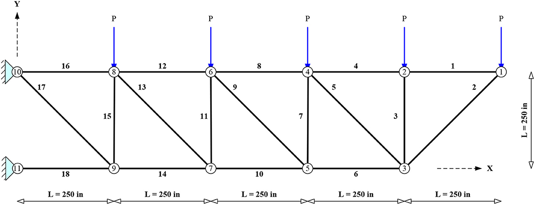
Figure 1. Planar 18-bar truss.

This problem has been solved in the literature either considering only sizing variables (Lee and Geem, 2004; Sonmez, 2011), or combining layout and sizing variables (Lamberti, 2008). Note that the truss is statically determinate, which means that the force acting in each bar is independent of the cross-sectional areas of the bars. The forces can be evaluated analytically using simple equilibrium equations (Charalampakis and Chatzigiannelis, 2018).

The optimization becomes more challenging if there are displacement constraints. The exact global optimum for a 6 in. tip displacement constraint and four-element groups (D = 4), obtained with the Cylindrical Algebraic Decomposition method, has been evaluated in Charalampakis and Chatzigiannelis (2018). This result is used as a target to evaluate the relative performance of metaheuristic methods by setting VTR = 9568.715 × 1.01 = 9664.402 lb.

Table S1 shows that all DE variants, EPSO, and SA practically converged to the analytical solution of the optimization problem, while HGA and ABC exhibited larger statistical dispersion. The average progress of the best solution, as well as the evolution of the success rate, are shown in Figure 2. It can be seen that EPSO and DE variants find the optimum region very quickly; 100% success rate is reached after only ~350D analyses. SA ranks next, requiring ~1250D analyses for 100% success whereas HGA reaches ~95% success at the end. Although it appears that ABC is not trapped into local optima, its progress is slow, and many structural analyses are required to obtain good results.

FIGURE 2

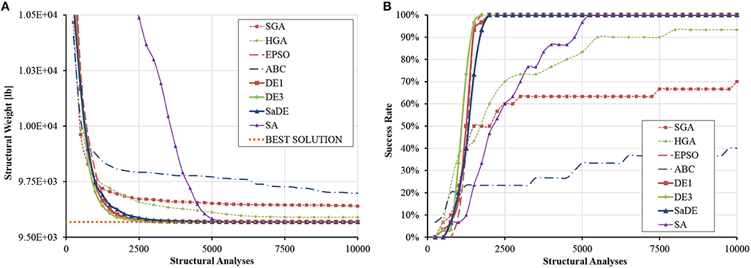
Figure 2. Size optimization of the planar 18-bar truss (A) average progress of the best solution (B) evolution of success rate.

25-Bar Tower (D = 8, SI = 7)

The spatial 25-bar tower with 10 nodes shown in Figure 3 has been studied extensively in the literature. The same material is used for all members (E = 10,000 ksi, ρ = 0.1 lb/in³). The cross-sectional area of each bar may vary between 0.01 and 35 in². Bars are grouped in eight groups (D = 8) with different compressive stress limit but the same tensile stress limit (see Table 1). In addition, displacements of top nodes 1 and 2 must be <0.35 in. in all directions. Two independent loading conditions are applied, as shown in Table 2.

FIGURE 3

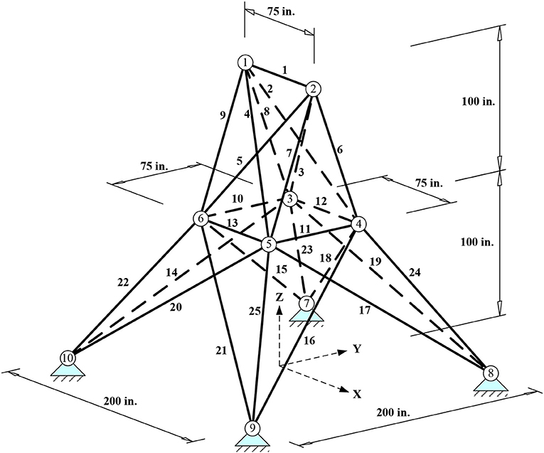
Figure 3. Spatial 25-bar tower.

TABLE 1

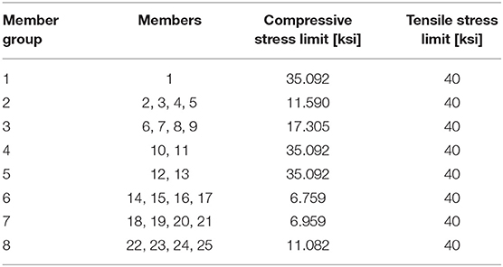
Table 1. Member grouping and stress limits for the spatial 25-bar tower.

TABLE 2

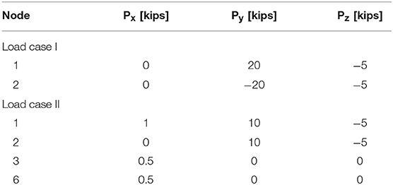
Table 2. Load cases for the spatial 25-bar tower.

Table S2 shows that DE1 and DE3 obtained the same best design, which is slightly better than the one found in literature in terms of weight [including MSPSO (Talatahari et al., 2013) by a very small margin]. This design was hence used as reference (VTR = 545.172 × 1.01 = 550.623 lb). The statistical data shown in Table S3 indicate that EPSO ranked right after DE in terms of best weight but was less robust than ABC and HGA. The average progress of the best solution and the variation of the success rate of each algorithm measured against the number of structural analyses are compared in Figure 4. It can be seen that DE1 and DE3 could reach 100% success after ~750D analyses, while SaDE follows at ~1250D analyses. SA, being the only method not employing a population of solutions but rather perturbing/improving a single solution, was the slowest to converge.

FIGURE 4

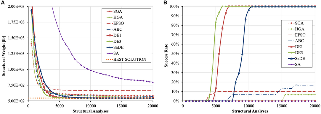
Figure 4. Size optimization of the spatial 25-bar tower (A) average progress of the best solution (B) evolution of success rate.

10-Bar Truss (D = 10, SI = 2)

Figure 5 shows the geometry and forces acting on a cantilever truss consisting of 10 bars and 6 nodes which has been analyzed by many researchers. Two loading cases are considered: in case I, P₁ = 100 kips and P₂ = 0; in case II, P₁ = 150 kips and P₂ = 50 kips. The same material is used for all members (E = 10,000 ksi and ρ = 0.1 lb/in³). The cross-sectional area of each bar may vary between 0.10 and 35 in². The stress limit is set to ±25 ksi, while the displacement of the free nodes must be limited to 2 in. in all directions.

FIGURE 5

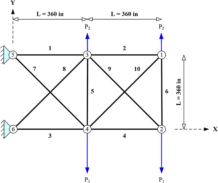
Figure 5. Planar 10-bar truss.

Regarding load case I, Table S4 shows that the best result was discovered by DE3 and used as reference (VTR = 5060.855 × 1.01 = 5111.464 lb). It is clear from Figure 6 that EPSO, DE1 and DE3 variants find the optimum region very quickly, as 100% success rate is reached after only ~500D analyses. SaDE follows next, producing very good results but with a slower convergence rate. Interestingly, SA may be the slowest to converge, but its final results are comparable to EPSO. HGA follows next, reaching ~60% at the end. The small difference between SGA and HGA during the first 10,000 analyses is due to the coarser discretization of the search space (16 and 10 bits per variable for SGA and HGA, respectively). The SSRM is triggered at 10,000 analyses while GDHC is introduced at 20,000 analyses, as shown in Figure 6A. Table S5 reveals the very small standard deviation of the results obtained by DE1 and DE3, as well as the small final ranges for all design variables.

FIGURE 6

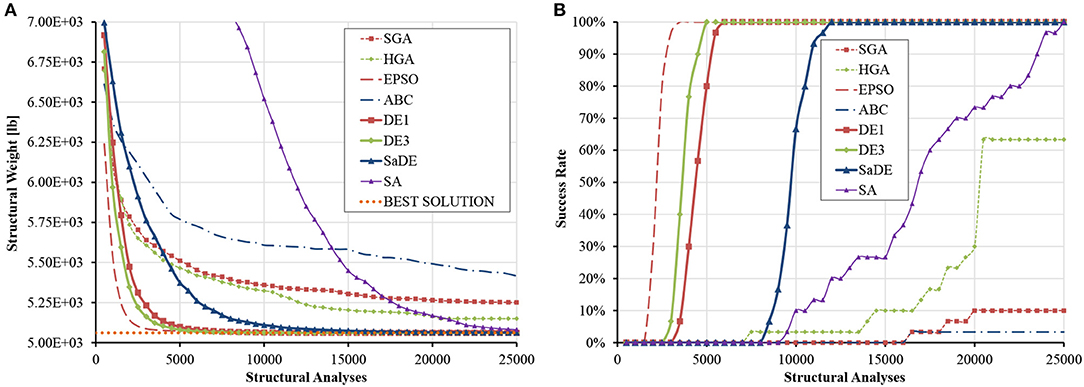
Figure 6. Size optimization of the planar 10-bar truss (load case I) (A) average progress of the best solution (B) evolution of success rate.

Regarding load case II, Table S6 shows that the best solution was discovered by DE3 and used as reference (VTR = 4676.932 × 1.01 = 4723.701 lb). The average progress of the best solution and the evolution of the success rate are presented in Figure 7, whereas a statistical analysis of the results is given in Table S7. The same conclusions can be drawn as in load case I. Once again, the final variable ranges for DE variants are very narrow.

FIGURE 7

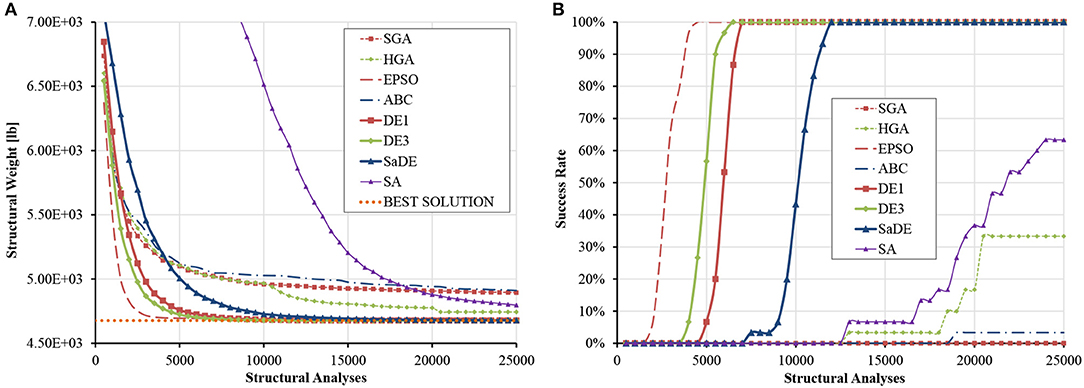
Figure 7. Size optimization of the planar 10-bar truss (load case II) (A) average progress of the best solution (B) evolution of success rate.

17-Bar Truss (D = 17, SI = 3)

The planar 17-bar with 9 nodes shown in Figure 8 has been studied in Berke and Khot (1987), Adeli and Kumar (1995), and Lee and Geem (2004). The same material is used for all members (E = 30000 ksi and ρ = 0.268 lb/in³). The structure is subject to a vertical force of 100 kips at node 9. The cross-sectional area of each bar may vary between 0.1 and 50 in². The stress limit is 50 ksi for both tension and compression, while the displacement of free nodes must be < ±2 in. Since no design variable linking was used, the problem dimensionality is D = 17.

FIGURE 8

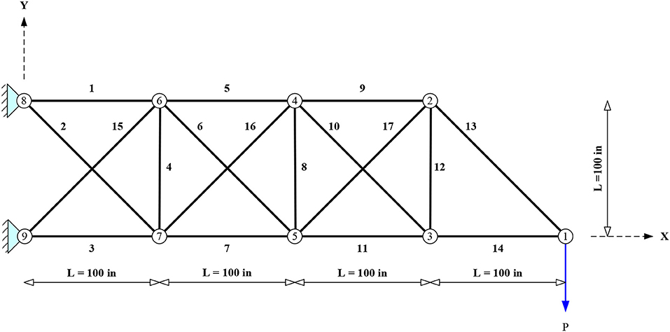
Figure 8. Planar 17-bar truss.

It can be seen from Table S8 that the best design was obtained by DE3. The corresponding structural weight was taken as target to compute VTR = 2581.895 × 1.01 = 2607.714 lb. The statistical data are given in Table S9 confirm the robustness of DE1 and DE3 that achieved a standard deviation on optimized weight equal to 0.047 and 0.086 lb, respectively, and converged practically to the same optimized weight. The other algorithms ranked in the following order: SaDE, EPSO, SA, HGA, and ABC.

The average progress of the best solution and the variation of the success rate of each algorithm with respect to the number of structural analyses are compared in Figure 9. It can be seen that DE1, DE3 could reach 100% success after ~900D analyses. SaDE also reached 100 success but much later. EPSO was the best algorithm in the early stages of the optimization process but about 20% of the runs failed to succeed at the end. SA achieved a 65% success rate when measured at the end of the analyses.

FIGURE 9

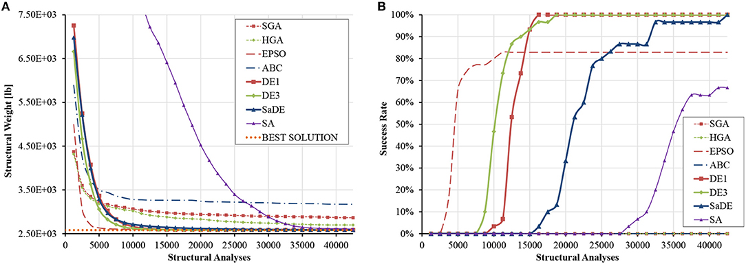
Figure 9. Size optimization of the planar 17-bar truss (A) average progress of the best solution (B) evolution of success rate.

200-Bar Truss (D = 29, SI = 50)

Figure 10 shows a planar 200-bar truss consisting of 200 bars and 77 nodes. The same material is used for all members (E = 30,000 ksi and ρ = 0.268 lb/in³). The structure is subjected to three independent loading conditions: (i) 1.0 kips acting in the positive x-direction at nodes 1, 6, 15, 20, 29, 34, 43, 48, 57, 62, and 71; (ii) 10 kips acting in the negative y-direction at nodes 1, 2, 3, 4, 5, 6, 8, 10, 12, 14, 15, 16, 17, 18, 19, 20, 22, 24, 26, 28, 29, 30, 31, 32, 33, 34, 36, 38, 40, 42, 43, 44, 45, 46, 47, 48, 50, 52, 54, 56, 57, 58, 59, 60, 61, 62, 64, 66, 68, 70, 71, 72, 73, 74, 75; (iii) the first two load cases acting together. Bars are linked in 29 groups (D = 29), as shown in Table 3, and their cross-sectional area may vary between 0.1 and 35 in². The structure is optimized with respect to limitations on member stresses that cannot exceed ±10 ksi; no displacement constraints are imposed.

FIGURE 10

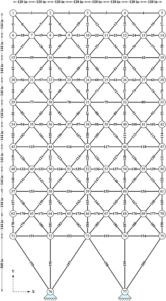
Figure 10. Planar 200-bar truss.

TABLE 3

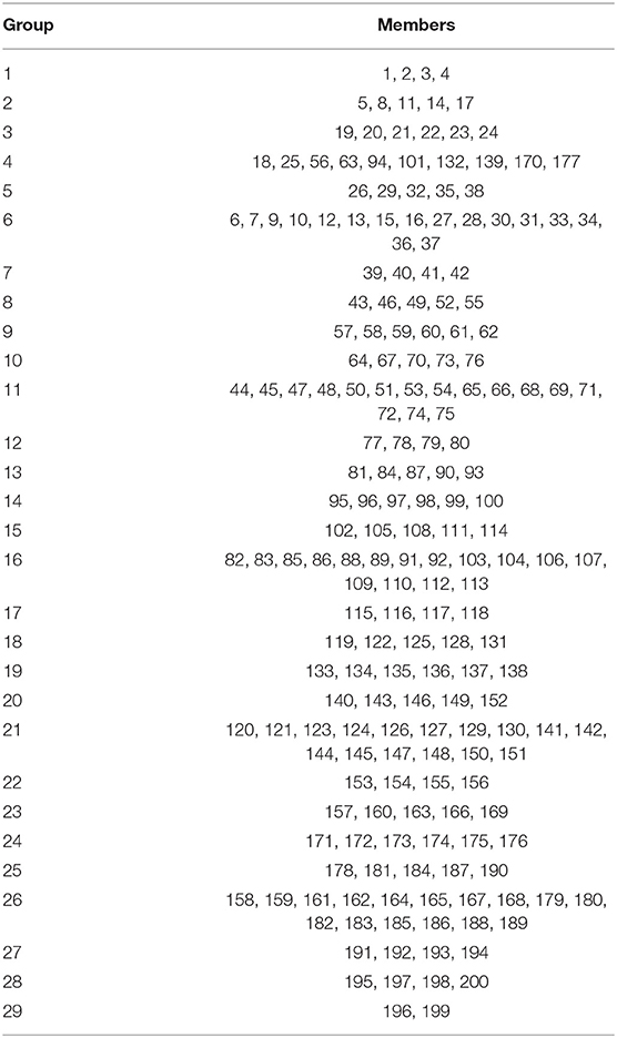
Table 3. Bar group members for the planar 200-bar truss (D = 29).

This optimization problem has been solved with both gradient-based and metaheuristic algorithms as an example of average-scale structure. Some optimum designs for this problem are presented in Table S10. Overall, the two best solutions were obtained by Coster and Stander (1996), although these designs slightly violate a few constraints. In order to correct this, cross-sectional areas of some element groups were increased by 0.001 in². The modified designs turned feasible and the VTR is computed as 25452.332 × 1.01 = 25706.855 lb.

The statistical data given in Table S11 indicate that DE variants are definitely superior over the other metaheuristic algorithms considered in this study. In particular, DE1 and DE3 converged to designs that are, on average, only 0.58–0.67% heavier than the target best design of Coster and Stander (1996), while SaDE produced designs that are, on average, 3.21% heavier. Remarkably, all DE variants exhibited at least one order lower standard deviations than the other algorithms. HGA ranked next in terms of average weight and standard deviation. ABC was comparable to HGA as far as best weight is concerned, but its standard deviation was more than three times larger. The average progress of the best design and the evolution of success rate with respect to the number of structural analyses are plotted in Figure 11 for all algorithms. SA shows an almost linear convergence rate, ranking last. It can be seen that only DE1 and DE3 reached a significant success rate, ranging between 85 and 90%, demonstrating excellent fine-tuning capabilities. SaDE barely missed producing successful runs, with the best design of 25794.837 lb achieved within 2500D analyses. Finally, Table S12 indicates that the superiority of DE3 is statistically very significant against all algorithms with the exception of DE1, with which no safe conclusion can be drawn.

FIGURE 11

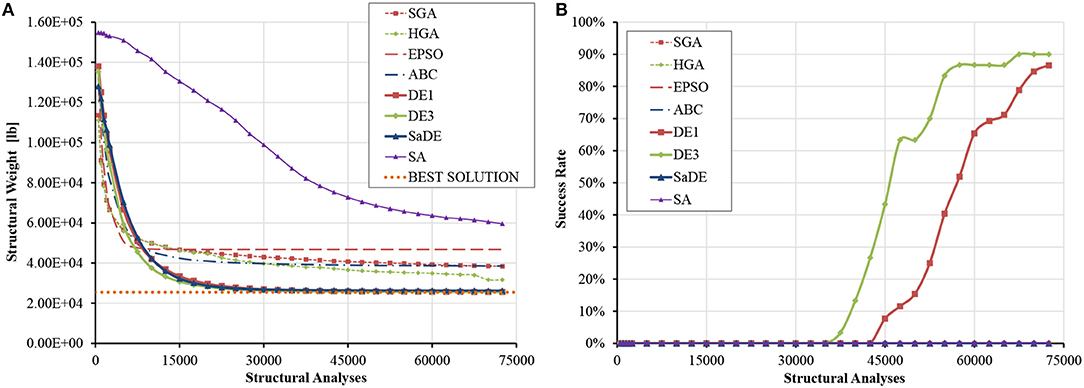
Figure 11. Size optimization of the planar 200-bar truss (D = 29) (A) average progress of the best solution (B) evolution of success rate.

200-Bar Truss (D = 200, SI = 50)

In order to compare the algorithms in a large-scale problem, the previously described planar 200-bar truss is re-examined without bar grouping; thus D = 200. Note that the best designs of the previous example are actually valid in this case as well, although not optimal anymore. Table S13 presents the statistical data gathered from optimization runs. It can be seen that the best design was found by DE1 (VTR = 21999.715 × 1.01 = 22219.712 lb); this design is quoted in Table S14. DE1 and DE3 were overall the best algorithms, followed by SaDE. Next comes ABC although the standard deviation of this algorithm was about 25% larger than that of HGA. The average progress of the best design measured against the number of structural analyses is shown in Figure 12A. It is confirmed that DE1 and DE3 are definitely superior over the other algorithms, exhibiting remarkable scalability with respect to problem dimensionality. SA again shows an almost linear convergence rate, which is not enough to surpass other algorithms within the selected computational budget. Figure 12B shows that success rate never exceeded 10%, because, for such a difficult problem, the VTR is too strict for a computational budget that increases linearly in D.

FIGURE 12

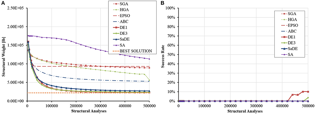
Figure 12. Size optimization of the planar 200-bar truss (D = 200) (A) average progress of the best solution (B) evolution of success rate.

Concluding Remarks

In this study the relative performance of variants of Genetic Algorithms (SGA, HGA), Particle Swarm Optimization (EPSO), ABC, Differential Evolution (DE1, DE3, and SaDE), and SA in sizing optimization problems of truss structures including up to 200 design variables was investigated. The comparison was based on a framework that is both unbiased and meaningful. In order to clearly assess the differences between algorithms, rigorous statistical analysis with large samples was used, based on common computational budget depended on the problem dimensionality, careful accounting for all function evaluations and monitoring of the success rate of each algorithm during the analyses.

Regarding the algorithms, SGA provides a baseline performance while the HGA, which combines a SSRM with a local optimizer, showed improved performance with respect to SGA. The difference became more clear for larger problems because of the relatively small chromosome length, as the coarse discretization appears to be very beneficial to the HGA. Refinement of the solutions is achieved through SSRM. The local search initiated 5,000 function evaluations before the end of each run. Except for the largest problem (200 bar truss with 200 design variables), the local optimum was usually found before the end of each run. The local search was invariably beneficial since the normal progress of the GA at this stage of optimization is usually very limited. Intermediate applications of the local search may improve performance; however, it is known that with GAs there is always the possibility of premature convergence when a single individual is much better than the other members of the population.

Simple PSO was tested in the preliminary versions of this study and produced very poor results; it was clear that the algorithm could not maintain a stable exploration/exploitation balance. Thus, an enhanced PSO algorithm (EPSO) was examined instead. It resulted very competitive in small to medium problems but failed in the larger problems. This is due to the scheme of Equation (14) employed to reduce maximum velocity and inertia factor. If h = 3 steps have passed without improving the global best position of the swarm, it is assumed that large velocities prevent progress due to overshooting. However, in large-scale problems, unjustified reduction of maximum velocity and inertia factor leads to search stagnation, as the particles literally freeze in place.

ABC is not easily trapped into local optima but has slow convergence because a single design variable is changed per mutant vector. The present results indicate that ABC could not compete with EPSO and DE variants in most test cases.

As far as it concerns DE variants, DE1 is based on rand/1/bin and DE3 is a stochastic mixture of rand/1/bin and best/1/bin. These variants combined particularly good convergence rate with robustness, stability, and scalability. DE3 showed improved convergence rate in the small-scale problems. A very greedy DE variant, based solely on best/1/bin, was also tested in the preliminary versions of this study and found to be very competitive only in small problems. Regarding SaDE, it appears that the advantage of its adaptive nature is traded-off by a small hysteresis (delay) in the convergence rate, as compared to DE1 and DE3. Note that the latter algorithms utilize fixed settings that were expected to work well based on the specific problem characteristics. This information may not be available for other problems, which makes SaDE and similar self-adapting algorithms a very good choice.

SA is the only method examined in this study which perturbs/improves a single solution. The lack of synergistic information within a population had the obvious effect that SA did not show explosive initial performance. Nevertheless, its progress was clear and it is evident that the Metropolis test (Equation 29) is a powerful method to escape local optima. For most of the small problems, this was enough to allow SA to rank among the best. For the planar 200-bar truss, the large dimensionality did not allow SA to compete within the strict computational budget. A more sophisticated control of the Boltzmann parameter than Equation (30) would improve its performance.

Overall, DE was superior over the rest of the algorithms and found very competitive designs, which in some cases were even better than those reported in the literature.

Data Availability Statement

All datasets generated for this study are included in the manuscript/Supplementary Files.

Author Contributions

AC had the research idea, drafted the article, and contributed to the numerical analysis of the examples and the statistical analysis of the results. GT contributed to the conception and design of the work, and interpretation of the results.

Conflict of Interest

The authors declare that the research was conducted in the absence of any commercial or financial relationships that could be construed as a potential conflict of interest.

Supplementary Material

The Supplementary Material for this article can be found online at: https://www.frontiersin.org/articles/10.3389/fbuil.2019.00113/full#supplementary-material

References

Adeli, H., and Kumar, S. (1995). Distributed Genetic Algorithm for structural optimization. J. Aerosp. Eng. 8, 156–163. doi: 10.1061/(ASCE)0893-1321(1995)8:3(156)

CrossRef Full Text | Google Scholar

Balling, R. J. (1991). Optimal steel frame design by Simulated Annealing. J. Struct. Eng. 117, 1780–1795. doi: 10.1061/(ASCE)0733-9445(1991)117:6(1780)

CrossRef Full Text | Google Scholar

Bellman, R. (1957). Dynamic Programming. Princeton, NJ: Princeton University Press.

Google Scholar

Berke, L., and Khot, N. S. (1987). “Structural optimization using optimality criteria,” in Computer Aided Optimal Design: Structural and Mechanical Systems, eds E. Atrek, R. H. Gallagher, K. M. Ragsdell, and O. C. Zienkiewicz (Berlin, Heidelberg: Springer), 271–311. doi: 10.1007/978-3-642-83051-8_7

CrossRef Full Text | Google Scholar

Bureerat, S., and Pholdee, N. (2016). Optimal truss sizing using an adaptive Differential Evolution algorithm. J. Comput. Civ. Eng. 30:04015019. doi: 10.1061/(ASCE)CP.1943-5487.0000487

CrossRef Full Text | Google Scholar

Camp, C. V. (2007). Design of space trusses using big bang–big crunch optimization. J. Struct. Eng. 133, 999–1008. doi: 10.1061/(ASCE)0733-9445(2007)133:7(999)

CrossRef Full Text | Google Scholar

Camp, C. V., and Farshchin, M. (2014). Design of space trusses using modified teaching–learning based optimization. Eng. Struct. 62–63, 87–97. doi: 10.1016/j.engstruct.2014.01.020

CrossRef Full Text | Google Scholar

Charalampakis, A. E. (2016). “Comparison of metaheuristic algorithms for size optimization of trusses,” in 11th HSTAM International Congress on Mechanics (Athens), 27–30.

Google Scholar

Charalampakis, A. E., and Chatzigiannelis, I. (2018). Analytical solutions for the minimum weight design of trusses by cylindrical algebraic decomposition. Arch. Appl. Mech. 88, 39–49. doi: 10.1007/s00419-017-1271-8

CrossRef Full Text | Google Scholar

Charalampakis, A. E., and Dimou, C. K. (2010). Identification of Bouc–Wen hysteretic systems using Particle Swarm Optimization. Comput. Struct. 88, 1197–1205. doi: 10.1016/j.compstruc.2010.06.009

CrossRef Full Text | Google Scholar

Charalampakis, A. E., and Dimou, C. K. (2015). Comparison of evolutionary algorithms for the identification of Bouc-Wen hysteretic systems. J. Comput. Civ. Eng. 29:04014053. doi: 10.1061/(ASCE)CP.1943-5487.0000348

CrossRef Full Text | Google Scholar

Charalampakis, A. E., and Koumousis, V. K. (2008). Identification of Bouc–Wen hysteretic systems by a hybrid evolutionary algorithm. J. Sound Vib. 314, 571–585. doi: 10.1016/j.jsv.2008.01.018

CrossRef Full Text | Google Scholar

Clerc, M., and Kennedy, J. (2002). The particle swarm - explosion, stability, and convergence in a multidimensional complex space. IEEE Trans. Evol. Comput. 6, 58–73. doi: 10.1109/4235.985692

CrossRef Full Text | Google Scholar

Coello, C. A. (2002). Theoretical and numerical constraint-handling techniques used with evolutionary algorithms: a survey of the state of the art. Comput. Methods Appl. Mech. Eng. 191, 1245–1287. doi: 10.1016/S0045-7825(01)00323-1

CrossRef Full Text | Google Scholar

Coello, C. A., and Christiansen, A. D. (2000). Multiobjective optimization of trusses using Genetic Algorithms. Comput. Struct. 75, 647–660. doi: 10.1016/S0045-7949(99)00110-8

CrossRef Full Text | Google Scholar

Coster, J. E., and Stander, N. (1996). Structural optimization using augmented Lagrangian methods with secant Hessian updating. Struct. Optim. 12, 113–119. doi: 10.1007/BF01196943

CrossRef Full Text | Google Scholar

Dede, T., and Ayvaz, Y. (2015). Combined size and shape optimization of structures with a new meta-heuristic algorithm. Appl. Soft Comput. 28, 250–258. doi: 10.1016/j.asoc.2014.12.007

CrossRef Full Text | Google Scholar

Degertekin, S. O. (2012). Improved harmony search algorithms for sizing optimization of truss structures. Comput. Struct. 92–93, 229–241. doi: 10.1016/j.compstruc.2011.10.022

CrossRef Full Text | Google Scholar

Degertekin, S. O., and Hayalioglu, M. S. (2013). Sizing truss structures using teaching-learning-based optimization. Comput. Struct. 119, 177–188. doi: 10.1016/j.compstruc.2012.12.011

CrossRef Full Text | Google Scholar

Dimou, C. K., and Koumousis, V. K. (2009). Reliability-based optimal design of truss structures using Particle Swarm Optimization. J. Comput. Civ. Eng. 23, 100–109. doi: 10.1061/(ASCE)0887-3801(2009)23:2(100)

CrossRef Full Text | Google Scholar

Eiben, A. E., and Smith, J. E. (2003). Introduction to Evolutionary Computing. New York: Springer. doi: 10.1007/978-3-662-05094-1

CrossRef Full Text | Google Scholar

Erol, O. K., and Eksin, I. (2006). A new optimization method: Big Bang–Big crunch. Adv. Eng. Softw. 37, 106–111. doi: 10.1016/j.advengsoft.2005.04.005

CrossRef Full Text | Google Scholar

Feury, C., and Geradin, M. (1978). Optimality criteria and mathematical programming in structural weight optimization. Comput. Struct. 8, 7–17. doi: 10.1016/0045-7949(78)90155-4

CrossRef Full Text | Google Scholar

Fourie, P. C., and Groenwold, A. A. (2002). The Particle Swarm Optimization algorithm in size and shape optimization. Struct. Multidiscip. Optim. 23, 259–267. doi: 10.1007/s00158-002-0188-0

CrossRef Full Text | Google Scholar

Geem, Z. W., Kim, J. H., and Loganathan, G. V. (2001). A new heuristic optimization algorithm: harmony search. Simulation 76, 60–68. doi: 10.1177/003754970107600201

CrossRef Full Text | Google Scholar

Hasançebi, O., and Azad, S. K. (2015). Adaptive dimensional search: a new metaheuristic algorithm for discrete truss sizing optimization. Comput. Struct. 154, 1–16. doi: 10.1016/j.compstruc.2015.03.014

CrossRef Full Text | Google Scholar

Hasançebi, O., Çarbaş, S., Dogan, E., Erdal, F., and Saka, M. P. (2009). Performance evaluation of metaheuristic search techniques in the optimum design of real size pin jointed structures. Comput. Struct. 87, 284–302. doi: 10.1016/j.compstruc.2009.01.002

CrossRef Full Text | Google Scholar

Holland, J. H. (1975). Adaptation in Natural and Artificial Systems. Ann Arbor, MI: University of Michigan Press.

Google Scholar

Karaboga, D., and Basturk, B. (2008). On the performance of Artificial Bee Colony (ABC) algorithm. Appl. Soft Comput. 8, 687–697. doi: 10.1016/j.asoc.2007.05.007

CrossRef Full Text | Google Scholar

Kaveh, A., Bakhshpoori, T., and Afshari, E. (2014a). An efficient hybrid particle swarm and swallow swarm optimization algorithm. Comput. Struct. 143, 40–59. doi: 10.1016/j.compstruc.2014.07.012

CrossRef Full Text | Google Scholar

Kaveh, A., and Ghazaan, M. I. (2015). A comparative study of CBO and ECBO for optimal design of skeletal structures. Comput. Struct. 153, 137–147. doi: 10.1016/j.compstruc.2015.02.028

CrossRef Full Text | Google Scholar

Kaveh, A., and Khayatazad, M. (2013). Ray optimization for size and shape optimization of truss structures. Comput. Struct. 117, 82–94. doi: 10.1016/j.compstruc.2012.12.010

CrossRef Full Text | Google Scholar

Kaveh, A., and Mahdavi, V. R. (2015a). Colliding bodies optimization for size and topology optimization of truss structures. Struct. Eng. Mech. 53, 847–865. doi: 10.12989/sem.2015.53.5.847

CrossRef Full Text | Google Scholar

Kaveh, A., and Mahdavi, V. R. (2015b). Two-dimensional colliding bodies algorithm for optimal design of truss structures. Adv. Eng. Softw. 83, 70–79. doi: 10.1016/j.advengsoft.2015.01.007

CrossRef Full Text | Google Scholar

Kaveh, A., Sheikholeslami, R., Talatahari, S., and Keshvari-Ilkhichi, M. (2014b). Chaotic swarming of particles: a new method for size optimization of truss structures. Adv. Eng. Softw. 67, 136–147. doi: 10.1016/j.advengsoft.2013.09.006

CrossRef Full Text | Google Scholar

Kaveh, A., and Talatahari, S. (2009a). Particle swarm optimizer, ant colony strategy and harmony search scheme hybridized for optimization of truss structures. Comput. Struct. 87, 267–283. doi: 10.1016/j.compstruc.2009.01.003

CrossRef Full Text | Google Scholar

Kaveh, A., and Talatahari, S. (2009b). Size optimization of space trusses using Big Bang–Big Crunch algorithm. Comput. Struct. 87, 1129–1140. doi: 10.1016/j.compstruc.2009.04.011

CrossRef Full Text | Google Scholar

Kaveh, A., and Talatahari, S. (2010). Optimal design of skeletal structures via the charged system search algorithm. Struct. Multidiscip. Optim. 41, 893–911. doi: 10.1007/s00158-009-0462-5

CrossRef Full Text | Google Scholar

Kaveh, A., and Zakian, P. (2014). Enhanced bat algorithm for optimal design of skeletal structures. Asian J. Civ. Eng. 15, 179–212. Available online at: https://ajce.bhrc.ac.ir/Portals/25/PropertyAgent/2905/Files/5878/179.pdf

Google Scholar

Kazemzadeh Azad, S., and Hasançebi, O. (2015). Computationally efficient discrete sizing of steel frames via guided stochastic search heuristic. Comput. Struct. 156, 12–28. doi: 10.1016/j.compstruc.2015.04.009

CrossRef Full Text | Google Scholar

Keane, A. J. (1996). “A brief comparison of some evolutionary optimization methods,” in Modern Heuristic Search Methods, eds. V. J. Rayward-Smith, I. H. Osman, C. R. Reeves, and G. D. Smith (Chichester: John Wiley), 255–272.

Google Scholar

Kennedy, J., and Eberhart, R. C. (1995). “Particle swarm optimization,” in IEEE International Conference on Neural Networks IV (Piscataway, NJ: IEEE Press), 1942–1948. doi: 10.1109/ICNN.1995.488968

CrossRef Full Text | Google Scholar

Kirkpatrick, S., Gelatt, C. D., and Vecchi, M. P. (1983). Optimization by Simulated Annealing. Sci. New Ser. 220, 671–680. doi: 10.1126/science.220.4598.671

PubMed Abstract | CrossRef Full Text | Google Scholar

Koumousis, V. K., and Georgiou, P. G. (1994). Genetic Algorithms in discrete optimization of steel truss roofs. J. Comput. Civ. Eng. 8, 309–325. doi: 10.1061/(ASCE)0887-3801(1994)8:3(309)

CrossRef Full Text | Google Scholar

Lamberti, L. (2008). An efficient Simulated Annealing algorithm for design optimization of truss structures. Comput. Struct. 86, 1936–1953. doi: 10.1016/j.compstruc.2008.02.004

CrossRef Full Text | Google Scholar

Lamberti, L., and Pappalettere, C. (2009). “An improved harmony-search algorithm for truss structure optimization,” in 12th International Conference Civil Structural and Environmental Engineering Computing, ed. B. H. V. Topping (Stirlingshire: Civil-Comp Press).

Google Scholar

Lee, K. S., and Geem, Z. W. (2004). A new structural optimization method based on the harmony search algorithm. Comput. Struct. 82, 781–798. doi: 10.1016/j.compstruc.2004.01.002

CrossRef Full Text | Google Scholar

Li, L. J., Huang, Z. B., Liu, F., and Wu, Q. H. (2007). A heuristic particle swarm optimizer for optimization of pin connected structures. Comput. Struct. 85, 340–349. doi: 10.1016/j.compstruc.2006.11.020

CrossRef Full Text | Google Scholar

Marano, G. C., Quaranta, G., and Monti, G. (2011). Modified Genetic Algorithm for the dynamic identification of structural systems using incomplete measurements. Comput. Civ. Infrastruct. Eng. 26, 92–110. doi: 10.1111/j.1467-8667.2010.00659.x

CrossRef Full Text | Google Scholar

Perez, R. E., and Behdinan, K. (2007). Particle swarm approach for structural design optimization. Comput. Struct. 85, 1579–1588. doi: 10.1016/j.compstruc.2006.10.013

CrossRef Full Text | Google Scholar

Press, W. H., Teukolsky, S. A., Vetterling, W. T., and Flannery, B. P. (2002). Numerical Recipes in C++: the Art of Scientific Computing. Cambridge: Cambridge University Press.

Google Scholar

Price, K. V., Storn, R. M., and Lampinen, J. A. (2005). Differential Evolution : a Practical Approach to Global Optimization. Berlin; Heidelberg: Springer-Verlag.

Google Scholar

Qin, A. K., Huang, V. L., and Suganthan, P. N. (2009). Differential Evolution algorithm with strategy adaptation for global numerical optimization. IEEE Trans. Evol. Comput. 13, 398–417. doi: 10.1109/TEVC.2008.927706

CrossRef Full Text | Google Scholar

Rajan, S. D. (1995). Sizing, shape, and topology design optimization of trusses using Genetic Algorithm. J. Struct. Eng. 121, 1480–1487. doi: 10.1061/(ASCE)0733-9445(1995)121:10(1480)

CrossRef Full Text | Google Scholar

Rao, R. V., Savsani, V. J., and Vakharia, D. P. (2011). Teaching–learning-based optimization: a novel method for constrained mechanical design optimization problems. Comput. Des. 43, 303–315. doi: 10.1016/j.cad.2010.12.015

CrossRef Full Text | Google Scholar

Ray, T., and Saini, P. (2001). Engineering design optimization using a swarm with an intelligent information sharing among individuals. Eng. Optim. 33, 735–748. doi: 10.1080/03052150108940941

CrossRef Full Text | Google Scholar

Rönkkönen, J., Kukkonen, S., and Price, K. V. (2005). “Real-parameter optimization with Differential Evolution,” in 2005 IEEE Congress on Evolutionary Computation (Edinburgh: IEEE), 506–513. doi: 10.1109/CEC.2005.1554725

CrossRef Full Text | Google Scholar

Schutte, J. F., and Groenwold, A. A. (2003). Sizing design of truss structures using particle swarms. Struct. Multidiscip. Optim. 25, 261–269. doi: 10.1007/s00158-003-0316-5

CrossRef Full Text | Google Scholar

Sonmez, M. (2011). Artificial Bee Colony algorithm for optimization of truss structures. Appl. Soft Comput. 11, 2406–2418. doi: 10.1016/j.asoc.2010.09.003

CrossRef Full Text | Google Scholar

Storn, R. M., and Price, K. V. (1997). Differential Evolution – a simple and efficient heuristic for global optimization over continuous spaces. J. Glob. Optim. 11, 341–359. doi: 10.1023/A:1008202821328

CrossRef Full Text | Google Scholar

Talatahari, S., Kheirollahi, M., Farahmandpour, C., and Gandomi, A. H. (2013). A multi-stage particle swarm for optimum design of truss structures. Neural Comput. Appl. 23, 1297–1309. doi: 10.1007/s00521-012-1072-5

CrossRef Full Text | Google Scholar

Wilke, D. N., Kok, S., and Groenwold, A. A. (2007). Comparison of linear and classical velocity update rules in Particle Swarm Optimization: notes on diversity. Int. J. Numer. Methods Eng. 70, 962–984. doi: 10.1002/nme.1867

CrossRef Full Text | Google Scholar

Wu, C.-Y., and Tseng, K.-Y. (2010). Truss structure optimization using adaptive multi-population Differential Evolution. Struct. Multidiscip. Optim. 42, 575–590. doi: 10.1007/s00158-010-0507-9

CrossRef Full Text | Google Scholar

Yang, Z., Tang, K., and Yao, X. (2008). “Self-adaptive Differential Evolution with neighborhood search,” in 2008 IEEE Congress on Evolutionary Computation (IEEE World Congress on Computational Intelligence) (Hong Kong: IEEE), 1110–1116. doi: 10.1109/CEC.2008.4630935

CrossRef Full Text | Google Scholar

Zhang, J., and Sanderson, A. C. (2009). JADE: adaptive Differential Evolution with optional external archive. IEEE Trans. Evol. Comput. 13, 945–958. doi: 10.1109/TEVC.2009.2014613

CrossRef Full Text | Google Scholar