Framework to Approximate the Value of Information of Bridge Load Testing for Reserve Capacity Assessment

Introduction

Civil infrastructure represents 30% of the annual global expenditure of the construction economy, evaluated at more than $10 trillion (World Economic Forum, 2016). Due to safe design and construction practices, infrastructure often has reserve capacity that is well above code requirements. An accurate reserve capacity assessment is challenging since the deterministic approach to estimate parameter values, which is suitable at the design stage, is not appropriate to assess existing structures (Hendy et al., 2016). Field measurements, collected through monitoring, help engineers improve assessments of reserve capacity of existing structures.

The interpretation of field measurements to improve knowledge of structural behavior is called structural identification (Catbas et al., 2013). To compare aging structure behavior with code load-carrying requirements, a model-based approach is usually necessary (Smith, 2016). In such cases, data from monitoring are used to improve model prediction accuracy when extrapolation is required. Model-free approaches are used only to perform behavior interpolation and the emergence of anomalies, such as the detection of structural degradation (Brownjohn et al., 2011).

The task of building behavior models, such as finite-element (FE) models, requires numerous assumptions, leading to several sources of uncertainties. The aim of structural identification is to improve knowledge on structural behavior and ultimately assess the structural safety through the estimation of reserve capacity. Most studies of structural identification have used either a residual-minimization strategy or the traditional Bayesian model updating (BMU) framework, which usually assume that uncertainties have zero-mean independent Gaussian forms (Beck and Katafygiotis, 1998; Katafygiotis and Beck, 1998; Lam et al., 2015). These assumptions are usually not compatible with the context of civil infrastructure since most modeling assumptions, such as idealized boundary conditions, present systematic uncertainties (Pasquier et al., 2014). Since little information is usually available, the estimation of correlation values between prediction errors is challenging and may influence the posterior parameter estimates (Simoen et al., 2013). To meet this challenge, traditional implementations of BMU must be modified, and this leads to complex formulations (Simoen et al., 2013; Pai et al., 2018). Several multiple-model approaches for structural identification have been developed using BMU (Dubbs and Moon, 2015), such as hierarchical BMU (Behmanesh et al., 2015) and parametrized BMU (Brynjarsdóttir and O'Hagan, 2014). While these approaches may be suitable for interpolation applications, such as damage detection, they are not suitable for extrapolation applications, such as reserve capacity assessments, due to the increase in uncertainty from hyper-parameterization (Li et al., 2016). Goulet and Smith (2013) presented a new structural identification methodology called error-domain model falsification (EDMF). Systematic uncertainties are explicitly taken into account in a way that is compatible with practical engineering knowledge (Pasquier and Smith, 2015). EDMF provides more accurate (albeit less precise) model-parameter identification when compared with traditional BMU and can be used for extrapolation applications (Proverbio et al., 2018c).

Measurements collected during load testing have been used to improve serviceability assessment (Goulet et al., 2010). Studies (Miller et al., 1994; Richard et al., 2010) involving destructive tests on reinforced concrete full-scale bridges show that non-linear finite-element models (NLFEA) are required to improve structural safety assessments involving ultimate limit states. Studies combining model calibration and NFLEA have been conducted (Zheng et al., 2009; Pimentel et al., 2010). However, they require the definitions of structural characteristics, such as constitutive laws of materials, that are seldom known precisely and are not directly related to the structural behavior during normal load conditions (Schlune et al., 2012; Cervenka et al., 2018). Recently, methodologies for reserve capacity assessments has been presented for full-scale case studies using a population-based probabilistic approach (Pai et al., 2018; Proverbio et al., 2018c). In these studies, only structural parameters that can be identified during load tests are updated while remaining parameters are taken to have conservative values as recommended by design guidelines. In addition, estimates include model uncertainties for prediction, and therefore conservative values of the reserve capacity are obtained.

The measurement system, usually designed by engineers using qualitative rules of thumb, influences directly the outcomes of structural identification. Quantitative studies on optimal sensor placement have been recently carried out to maximize the information gain for bridge load testing. The sensor placement task is usually seen as a discrete optimization task. As the number of possible sensor configurations increases exponentially with the number of sensors and locations, most studies have used a sequential search (greedy algorithms) to reduce the computational effort (Kammer, 2005). Most researchers have used a sensor placement objective function that selects sensor locations based on their expected information content, such as maximizing the determinant of Fisher information matrix (Udwadia, 1994; Heredia-Zavoni and Esteva, 1998), minimizing the information entropy in posterior model-parameter distribution (Papadimitriou et al., 2000; Papadimitriou, 2004; Papadimitriou and Lombaert, 2012; Argyris et al., 2017), and maximizing information entropy in multiple-model predictions (Robert-Nicoud et al., 2005a).

To reduce the redundancy in sensor location information content when multiple sensors are used, the concept of joint entropy was introduced (Papadopoulou et al., 2014) using a hierarchical algorithm. This algorithm was extended to account for mutual information between sensor types and static load tests (Bertola et al., 2017). Although information gain is critical, the definition of the optimal sensor configuration must include multiple performance criteria, such as cost of monitoring and the robustness of information gain to test hazards. Recently, a comprehensive framework to design measurement system based on a multi-criteria decision analysis (MCDA) was presented (Bertola et al., 2019). This study shows that the best measurement system depends on asset-manager preferences. However, the influence of the expected monitoring outcomes to support asset managers during reserve capacity assessment was not investigated.

Information collected during monitoring comes at a cost that may not be justified by its influence on asset manager actions. The value of information (VoI) is a measure of how information benefits decision making under uncertainty (Raiffa and Schlaifer, 1961). Within Bayesian Frameworks, VoI has been extensively used to evaluate the benefit of structural health monitoring systems (SHM) (Straub et al., 2017). The principal limitation is that VoI estimation is computationally expensive (Straub, 2014). Quantitative frameworks have been proposed (Pozzi et al., 2010; Zonta et al., 2014; Thöns, 2018). Nevertheless, they used only idealized structural systems, reducing their practical applications. Additionally, many applications have been proposed for maintenance and operations over time based on Bayesian dynamic networks (BDN) (Weber et al., 2012; Luque and Straub, 2016) or partially-observable Markov decision process (POMDP) (Ellis et al., 1995; Papakonstantinou and Shinozuka, 2014a,b). POMDP methodologies have been extended for multi-element systems (Fereshtehnejad and Shafieezadeh, 2017) and continuous and non-linear states (Schöbi and Chatzi, 2016). However, most studies have been performed assuming that each system component behaves independently (Li and Pozzi, 2019). Including system-level interactions that are present in practical applications generates additional computational challenges.

Additionally, VoI has been used as an objective function for sensor-placement tasks and shown to provide better configurations than independent entropy-based objective functions (Malings and Pozzi, 2016a). A disadvantage of using the VoI as a sensor placement objective function is again the long computation times (Malings and Pozzi, 2016b). Additionally, greedy approaches that are used in the optimization task of sensor placement may lead to sub-optimal decisions since the VoI metric is not submodular (Malings and Pozzi, 2019).

For structural identification purposes, the task differs from operation and maintenance as it is not time-dependent. Methodologies developed for operation and maintenance of infrastructure, such as POMDP, are thus not suitable. A methodology to select the optimal sequence of measurements and intervention actions based on pre-posterior analysis and using a greedy search was presented for a simplified structure (Goulet et al., 2015). For a full-scale case study, the expected identifiability of parameter values and prediction ranges was proposed based on simulated measurements and the EDMF framework (Goulet and Smith, 2012). The work was extended in Pasquier et al. (2017) to quantify the expected utility of measurement systems for remaining fatigue life estimations. However, this methodology is applicable only to fast critical reserve capacity calculations, such as remaining fatigue life.

This paper presents a framework to evaluate the VoI of load testing for reserve capacity assessment for several limit states on a full-scale case study. The aim is to determine if the information collected during monitoring at a given cost is justified by its potential to influence asset managers in their decisions. As this framework is based on EDMF rather than traditional BMU, the approach to estimate the expected information gain of monitoring differs significantly (Bertola et al., 2017). This means that traditional VoI quantifications must be adapted. Additionally, a new approach by levels of approximation is employed to prevent unnecessary computationally expensive VoI analyses when faster upper bound estimations may be sufficient to reject the hypothesis that monitoring is useful. The design approach where the detail level of an analysis increases only when more accurate predictions are necessary, such as in Muttoni et Fernandez (Muttoni and Ruiz, 2012), for structural design. This approach provides a practical strategy in the assessment of the VoI of bridge load testing when decisions require complex reliability analyses. In cases where load testing is appropriate, VoI helps select alternatives of measurement systems (Bertola et al., 2019), where the expected information gain is estimated using the joint entropy objective function.

The study is organized as follows. Background methodologies which are necessary to the understanding of the paper are first presented in section Background. Section Level-of-Approximation Approach to Evaluate the Value of Information of Bridge Load Testing for Reserve-Capacity Assessment shows the framework to evaluate the value of information of bridge load testing for reserve capacity assessment using a level of approximation approach. Results in terms of value of information of multiple measurement system scenarios of a full-scale case study are then provided in section Case Study and results are discussed in section Discussion.

Background

In this section, background methodologies that are necessary for the understanding of this study, are presented. First, the structural identification methodology, called error-domain model falsification, is presented. Then, the sensor placement algorithm for static measurements, called hierarchical algorithm, is described.

Structural Identification—Error-Domain Model Falsification

Error-domain model falsification (EDMF), is an easy-to-use methodology for structural identification (Goulet and Smith, 2013). A population of behavior model instances are generated, and their predictions are compared with field measurements in order to identify plausible model instances of a parameterized model class.

At a sensor location i, model predictions g_k(i,Θ_k) are generated by assigning a vector of parameter values Θ_k. The model class involves a finite element parametric model that includes characteristics, such as material properties, geometry, boundary conditions, and excitations, as well as the quantification of both model (U_i,gk) and measurement (U_i,ŷ) uncertainties. The real structural response R_i, that is unknown in practice, is linked to the measured value ŷ_i at sensor location i among n_y monitored locations using Equation (1).

$\begin{array}{ll}{g}_k(i,{\Theta }_k)+U_{i,g_k}=R_i={\widehat{y}}_i+U_{i,\widehat{y}}\forall i\in \left\{1,\dots ,n_y\right\}& (1)\end{array}$

Following Robert-Nicoud et al. (2005c), U_i,gk and U_i,ŷ are combined in a unique source U_i,c using Monte-Carlo sampling. Equation (1) is then transformed in Equation (2), where the residual r_i quantifies the difference between the model prediction and the field measurement at a sensor location i.

$\begin{array}{ll}{g}_k(i,{\Theta }_k)-{\widehat{y}}_i=U_{i,c}=r_i& (2)\end{array}$

In EDMF, plausible models are selected by falsifying instances for which residuals exceed threshold bounds, given combined uncertainties and a target reliability of identification. First the target of reliability ϕ is fixed. Traditionally, a value of 95% is taken (Goulet and Smith, 2013). The Šidák correction (Šidák, 1967), is used to maintain a constant level of confidence when multiple measurements are compared to model-instance predictions. Then, threshold bounds, t_i,low and t_i,high are calculated using Equation (3). These bounds express the shortest intervals through the probability density function (PDF) of combined uncertainties f_Ui(u_i) at a measurement location i, including the probability of identification ϕ.

$\begin{array}{ll}{\forall i=1,\dots ,n_y:\varphi }^{1/n_y}={\displaystyle {\int }_{u_{i,low}}^{u_{i,high}}}{f}_{U_i}(u_i)d{u}_i& (3)\end{array}$

The candidate model set is defined using Equation (4), where ${\Omega }_k^{″}$ is the candidate model set (CMS) built of unfalsified model instances. Candidate models are set to be equally likely since little information is usually available to describe the combined uncertainty distribution (Robert-Nicoud et al., 2005b). Thus, they are assigned an equal probability, while falsified model instances are assigned a null probability.

$\begin{array}{ll}{\Omega }_k^{″}=\{{\theta }_k\in {\Omega }_k|\forall i\in \{1,\dots ,n_y\}{t}_{i,low}\le g_k\left(i,{\Theta }_k\right)-{\widehat{y}}_i\le t_{i,high}\}& (4)\end{array}$

If all model instances are falsified, this means that no model predictions are compatible with measurements given uncertainty sources. This situation can happen if the initial model instance set does not effectively reflect the true behavior. Provided that the initial sampling is adequate, this means that the model class is not correct. In such cases, the data interpretation using EDMF leads to reevaluation of assumptions and a new model class is generated (Pasquier and Smith, 2016), which is an important advantage of EDMF compared with other structural identification approaches.

Sensor-Placement Algorithm—Hierarchical Algorithm

A measurement system design framework is used to rationally select the appropriate measurement system when structural information is incomplete. The first step involves building the numerical model and selecting the model class. Then, prediction data from a population of model instances are generated using a sampling procedure. This prediction set is the typical input to evaluate expected information gained by sensor locations using a sensor placement algorithm. The optimal measurement system is then defined using a multi-criteria approach, taking into account multiple performance criteria, such as information gain and cost of monitoring as well as asset manager preferences.

Information entropy was introduced as a sensor-placement objective function for system identification by Papadimitriou et al. (2000). At each sensor location i, the range of model instance predictions is subdivided into N_I,i intervals. The interval width is evaluated using combined uncertainty U_i,c(Equation 2) (Robert-Nicoud et al., 2005a). The probability that model instance prediction g_i,j falls inside the jth interval is equals to $P(g_{i,j})=\frac{m_{i,j}}{\sum m_{i,j}}$, where m_i,j is the number of model instances falling inside this specific interval. The information entropy H(g_i) is evaluated at a sensor location i using Equation (5).

$\begin{array}{ll}H\left(g_i\right)=-{{\displaystyle \sum }}_{j=1}^{N_{I,i}}P\left(g_{i,j}\right)\text{ lo}{\text{g}}_{2}P\left(g_{i,j}\right)& (5)\end{array}$

Sensor locations with high values for H(g_i) are attractive locations since sensors are most effective when placed in locations that have high disorder in model-instance predictions. When physics-based systems are monitored, measurements are typically correlated. To assess the redundancy of information gain between sensor locations, joint entropy as new objective function was proposed by Papadopoulou et al. (2014). Joint entropy H(g_i,i+1) assesses the information entropy amongst sets of predictions to account for mutual information between sensors. For a set of two sensors, the joint entropy is calculated using Equation (6), where P(g_i,j, g_{i+1, k}) is the joint probability that model instance predictions falls inside the jth interval at sensor i and the kth interval at sensor i+1.

$\begin{array}{ll}H\left(g_{i,i+1}\right)=-{{\displaystyle \sum }}_{k=1}^{N_{I,i+1}}{{\displaystyle \sum }}_{j=1}^{N_{I,i}}P\left(g_{i,j},g_{i+1,k}\right)\text{ lo}{\text{g}}_{2}P\left(g_{i,j},g_{i+1,k}\right)& (6)\end{array}$

where k ∈ {1, …, N_I,i+1} and N_I,i+1 is the maximum number of prediction intervals at the i+1 location and i + 1 ∈ {1, …, n_s} with the number of potential sensor locations n_s. Due to the redundancy in information gain between sensors, the joint entropy is less than or equal to the sum of the individual information entropies. Equation (7) can be rewritten as Equation (10), where I(g_i,i+1) is the mutual information between sensor i and i+1.

$\begin{array}{ll}H\left(g_{i,i+1}\right)=H\left(g_i\right)+H\left(g_{i+1}\right)-I\left(g_{i,i+1}\right)& (7)\end{array}$

If multiple static load tests are performed, mutual information at a sensor location i occurs between the measurements, as it does between sensors. The hierarchical algorithm is an optimization strategy introduced by Papadopoulou et al. (2014) to calculate the joint entropy of sensor configurations in a reasonable computational time, following a greedy-search strategy. This algorithm was adapted to take into account mutual information between static load tests (Bertola et al., 2017) as well as dynamic data (Bertola and Smith, 2019).

Bertola et al. (2019) have proposed a multi-objective approach for measurement system design. Five conflicting performance criteria are taken into account to recommend a measurement system: information gain, cost of monitoring, sensor installation, ability to detect outliers, and robustness of information gain in case of the best sensor failure. Recommendations are made based on asset manager preferences and is found using the SMAA-PROMETHEE methodology (Corrente et al., 2014).

Level-Of-Approximation Approach to Evaluate the Value Of Information of Bridge Load Testing for Reserve Capacity Assessment

In this section, a framework that assesses the value of information of bridge load testing for reserve capacity estimation using an approach by levels of approximation is presented. The first section provides an overview of the framework. Then, each step of the framework is presented in detail throughout the following sections.

Framework Presentation

The reserve capacity (RC) of existing bridges is usually defined as the additional carrying capacity compared with code requirements for a specific limit state. When traffic loading is the leading action, the reserve capacity is the ratio between the carrying capacity of the structural system using a conservative approach Q_cons and the code traffic load Q_d.

For existing structures, reserve capacity is usually assessed after monitoring. First, structural identification is conducted and parameter values Θ_CMS that most influence the model predictions at the test conditions are identified. The reserve capacity estimation is an extrapolation task; values for parameters at test conditions may not be representative of the behavior at ultimate limit state loading conditions. For example, boundary conditions, such as pinned supports may have rotational rigidity during load tests. This rigidity cannot be used to calculate conservative estimates of reserve capacity at the ultimate limit state. Therefore, a subset of the plausible parameter values obtained under load test conditions Θ_CMS,LS is taken into account for the estimation of ultimate carrying capacity of the structural system Q(Θ_CMS,LS). Remaining parameters influencing the reserve capacity that cannot be identified during load testing are taken to have design values. Reserve capacity is then assessed using Equation (8). Prior to measurements, the value of reserve capacity estimated after monitoring RC(Θ_CMS,LS) is thus unknown.

$\begin{array}{ll}RC({\Theta }_{CMS,LS})=\frac{Q({\Theta }_{CMS,LS})}{Q_d}& (8)\end{array}$

The value of information (VoI) quantifies the amount of money asset managers are willing to pay for information prior making a decision. In this study, the VoI is used to evaluate the influence of load-testing information on asset manager decisions related to reserve capacity assessment. The VoI is calculated using Equation (9) (Zonta et al., 2014), where C_{prior monitoring} is the action cost if no monitoring information is available and C_{after monitoring} is the cost of actions after monitoring.

$\begin{array}{ll}VoI=C_{priormonitoring}-C_{aftermonitoring}& (9)\end{array}$

Prior to monitoring, the bridge is assumed to present insufficient reserve capacity (RC(Θ_CMS,LS) < 1), and the C_{prior monitoring} is equal to the cost of intervention C_int, where int stands for intervention. C_int is assumed to be the lowest possible cost of interventions that could include either structural improvements, load reduction, or better load definition.

Information collected during load testing may influence reserve capacity assessments through the identification of unknown model parameter values (Equation 8), and this can modify asset managers operational costs after monitoring. C_{after monitoring} includes possible asset manager decisions after monitoring associated with their probability of occurrence as well as the cost of monitoring. In this study, a simple binary scheme of possible asset manager decisions is assumed. If the bridge presents a reserve capacity (RC(Θ_CMS,LS) ≥ 1) after monitoring, no action is required and a “do nothing” scenario, with an associated cost of C_not, is preferred. If the bridge does not have reserve capacity (RC(Θ_CMS,LS) < 1), asset managers proceed to interventions with the unchanged associated cost C_int.

When the bridge RC is assessed using load testing, the VoI for a given limit state is influenced by three factors: i) the amount of money saved (C_int − C_not) by avoiding unnecessary interventions when monitoring reveals a reserve capacity; ii) the probability of finding RC(Θ_CMS,LS) ≥ 1 after monitoring, called P(RC⁺) and iii) costs of monitoring C_mon. Equation (9) is consequently rewritten in Equation (10). Asset managers are willing to cover monitoring expenses only if expected savings exceed monitoring costs. Monitoring is recommended when VoI > 0, while VoI < 0 suggests that interventions should proceed without monitoring.

$\begin{array}{ll}VoI={\left(C_{int}-C_{not}\right)}^{*}P\left(R{C}^{+}\right)-C_{mon}& (10)\end{array}$

With,

$\begin{array}{ll}P\left(R{C}^{+}\right)\equiv ProbabilitythatRC\left({\Theta }_{CMS,LS}\right)\ge 1aftermonitoring& (11)\end{array}$

The estimation of P(RC⁺) is computationally expensive. For instance, this estimation requires the evaluation of the expected information gain of monitoring using a measurement system design methodology. Additionally, the influence of model parameters on reserve capacity assessments using FE model predictions is needed. Nevertheless, upper bounds of P(RC⁺), corresponding to upper bounds of VoI, can be computed. These upper bounds are assessed using optimistic estimates of model instance discriminations and reserve capacity assessments.

The level of approximation is a design approach where the level of detail of an analysis increases only when more accurate predictions are necessary. For example, see Muttoni et Fernandez for structural design (Muttoni and Ruiz, 2012). In the case of structural design, if a simple conservative model provides a lower bound of load capacity that already fulfills code requirements, no further analysis is needed and engineers avoid the costs of building detailed models.

Figure 1 presents the level-of-approximation (LoA) approach for RC assessment using bridge load testing. Four levels are depicted, where the accuracy of the VoI estimation and the time devoted to the analysis increases with the LoA. In the first three LoAs, an upper bound of P(RC⁺) is estimated. Therefore, each LoA represents an upper bound estimation of the VoI of monitoring. For example, in LoA 1, a perfect model instance discrimination is assumed, and no uncertainties are included in the reserve capacity assessment. Due to these assumptions, the value of ${P\left(R{C}^{+}\right)}_{LoA1}$ is overestimated. When increasing the level of approximation, less optimistic assumptions are involved and thus P(RC⁺) decreases and becomes more accurate. As other assumptions are reevaluated in each LoA, the framework must be performed until LoA 4 is reached to confirm that monitoring is recommended. When the computed VoI is negative despite using an upper bound estimation, no monitoring should be performed and increasing prediction accuracy is meaningless. If VoI > 0, the next step of the estimation of the VoI should be performed, requiring additional information and increasing the cost of the analysis.

FIGURE 1

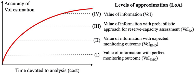
Figure 1. Accuracy of the value of information (VoI) estimation of bridge load testing for reserve capacity assessment as function of time devoted to the analysis.

The inequality VoI > 0 is rearranged in Equation (12). The left-hand side corresponds to the ratio between cost savings and costs of monitoring, called the $\frac{potentialbenefit}{cost}$ ratio, and must be larger than the inverse of P(RC⁺)to justify monitoring. As this ratio is typically an input of the analysis, the estimation of $\frac{1}{P\left(R{C}^{+}\right)}$ provides a threshold of the minimum $\frac{potentialbenefit}{cost}$ ratio to justify load testing.

$\begin{array}{ll}\frac{C_{int}-C_{not}}{C_{mon}}>\frac{1}{P\left(R{C}^{+}\right)}& (12)\end{array}$

To illustrate the potential of the framework, three scenarios are presented in Figure 2 along with their assessments of probability and benefit-cost ratios. In the first scenario, the upper bound of P(RC⁺), calculated in LoA 1, leads to the conclusion that the benefit-cost ratio does not justify monitoring. Therefore, the analysis stops and interventions should proceed without monitoring. For the second scenario, the benefit-cost ratio is significantly larger than $\frac{1}{P\left(R{C}^{+}\right)}$ after the first LoA. The second LoA of VoI is thus performed and a new upper bound of $\frac{1}{P\left(R{C}^{+}\right)}$ is calculated, leading to the conclusion that monitoring is not justified. In this scenario, the analysis terminates with LoA2 and monitoring is not recommended. In the third scenario, the VoI estimation is performed until the fourth level, which corresponds to the most accurate estimation of P(RC⁺). As the true benefit-cost ratio of this scenario is larger than the threshold given by $\frac{1}{P\left(R{C}^{+}\right)}$, monitoring is recommended.

FIGURE 2

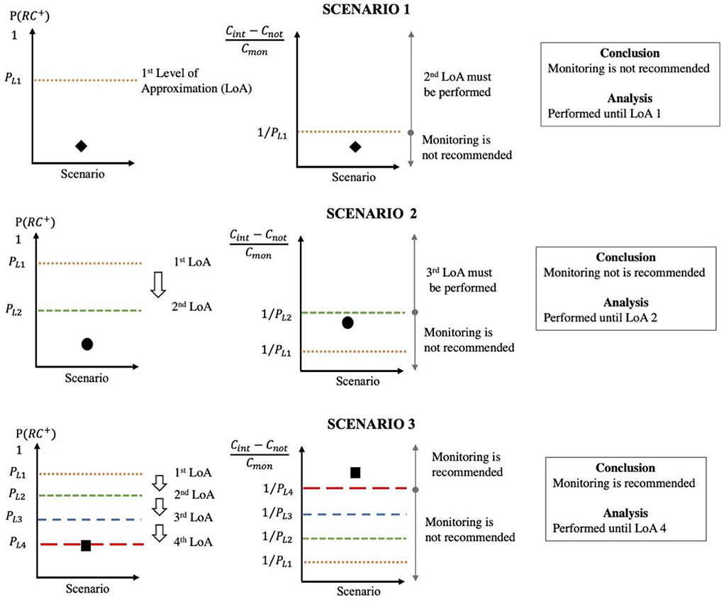
Figure 2. Illustrative scenarios of the level of approximation approach to evaluate the minimum benefit–cost ratio $\frac{C_{int}-C_{not}}{C_{mon}}$ that justifies monitoring.

Figure 3 shows the framework to evaluate the VoI of bridge load testing. Each step of the framework is described in detail in subsections below. The task definition involves generating the structural behavior model, selecting model parameters that influence predictions, defining possible measurement systems and critical limit states. The aim of preliminary RC assessments is to evaluate if the load testing can influence the structural-safety assessment. If this condition is fulfilled, the RC is estimated according to the level of approximation strategy described in Figure 1. The first three levels evaluate an upper bound of VoI. Therefore, the if VoI < 0, interventions are necessary. LoA1 [section LoA 1—Value of Information With Perfect Monitoring Outcome (VoI_PMO)] requires generation a population of model instances with predictions of reserve capacity. This level involves the assumption of perfect distinction of model instances and provides a simple RC assessment. LoA2 [section LoA 2—Value of Information With Expected Monitoring Outcome (VoI_EMO)] includes a measurement system design framework to evaluate the expected information gain using additional information of model instance predictions under test conditions. LoA3 [section LoA 3—Value of Information With a Probabilistic Approach for Reserve-Capacity assessment (VoI_PA)] involves a probabilistic approach to assess the population-based RC, while the fourth level includes uncertainties related to the monitoring into the estimation of the VoI. LoA4 [section LoA 4—Value of Information (VoI)] presents an accurate VoI estimation, based on the probabilistic definition of the P(RC⁺), while lower LoAs involve more approximate assessments. Based on the VoI distribution, hypothesis testing is introduced to determine whether monitoring provides effective support to decision making. In case VoI > 0, is it thus recommended to monitor the structure, while if VoI < 0 interventions are needed. A detailed description of each step of the framework is provided below.

FIGURE 3

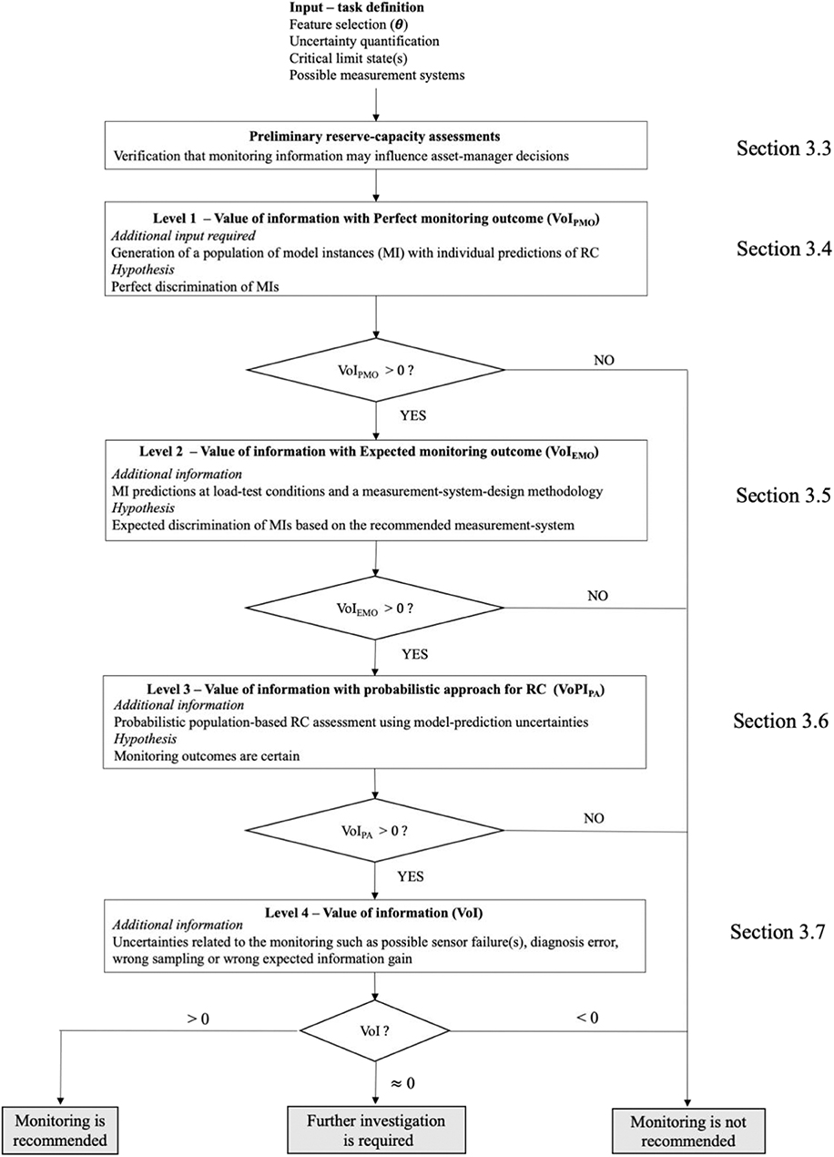
Figure 3. Framework of the evaluation of the value of information of bridge load testing for reserve capacity estimation based on a level of approximation approach.

Task Definition

This section describes the preliminary steps that are required before performing the structural identification task. The physics-based model of the structure is constructed and analyzed to obtain quantitative predictions of structural behavior, such as deflections under load test conditions and reserve capacity estimations. Model parameters that have the highest impact on predictions are selected based on a sensitivity analysis. Significant non-parametric uncertainties are usually involved as the results of geometrical and mathematical simplifications are present in the FE model. These uncertainties must be estimated as they influence the structural-identification outcome.

Load testing conditions, such as the bridge excitation, available sensor types, the number of sensors, and their possible locations are chosen by engineers. Eventually, critical limit states are selected and the costs of intervention for each specific scenario are estimated. Altogether, these preliminary steps allow the evaluation of the value of information of the bridge load testing for reserve capacity assessment.

Preliminary Reserve Capacity Assessments

This section describes the initial calculation of reserve capacity. The aim is to evaluate whether the information collected during the load testing influences the RC assessment. For monitoring to be worthwhile, two conditions are necessary. When conservative parameter values Θ_cons are assumed, the calculated reserve capacity is expected to be lower than 1 (Equation 13). On the contrary, when optimistic model parameter values Θ_opt–taken as upper bounds of model-parameter ranges—are assumed, values of reserve capacity >1 are expected (Equation 14). The first condition implies that, for the current level of knowledge, the bridge does not satisfy code requirements. Structural improvements are thus necessary. The second condition implies that the outcome of the bridge load testing may help avoid unnecessary interventions by revealing hidden sources of reserve capacity.

$\begin{array}{ll}RC\left({\Theta }_{cons}\right)=\frac{Q_{max}\left({\Theta }_{cons}\right)}{Q_d\left({\gamma }_Q\right)}<1& (13)\end{array}$

$\begin{array}{ll}RC\left({\Theta }_{opt}\right)=\frac{Q_{max}\left({\Theta }_{opt}\right)}{Q_d\left({\gamma }_Q\right)}>1& (14)\end{array}$

LoA 1—Value of Information With Perfect Monitoring Outcome (VoI_PMO)

In this section, the ${P\left(R{C}^{+}\right)}_{LoA1}$ is estimated. First, a population of model instances is generated using traditional sampling techniques. Each model instance has a unique set of model parameter values that influence model predictions. In this section, two assumptions are made. First, the measurement system is assumed to perfectly differentiate model instances (assumption of perfect monitoring outcome), which implies that the CMS will consist of a single model instance after monitoring. Then, the reserve capacity is assessed using this unique candidate model. As the outcome of the monitoring is unknown (i.e., which model instance will be identified), the ${P\left(R{C}^{+}\right)}_{LoA1}$ depends on the ratio between the number of model instances $n_{MI}\left(R{C}^{+}\right)$ having RC(Θ_MI,LS) ≥ 1 over the total number of model instances n_MI. The VoI_PMO is calculated using Equation (15), which includes an estimation of the monitoring cost C_mon. This estimation is an upper bound of the true value of information. If VoI_PMO < 0, the cost of monitoring is not justified by the benefit-cost ratio. Therefore, monitoring should not be performed. If VoI_PMO > 0, the analysis of LoA 2 is required.

$\begin{array}{ll}Vo{I}_{PMO}={\left(C_{int}-C_{not}\right)}^{*}{P(R{C}^{+})}_{LoA1}-C_{mon}& (15)\end{array}$

with,

$\begin{array}{ll}{P\left(R{C}^{+}\right)}_{LoA1}=\frac{n_{MI}\left(RC\left({\Theta }_{MI,LS}\right)\ge 1\right)}{n_{MI}}& (16)\end{array}$

LoA 2—Value of Information With Expected Monitoring Outcome (VoI_EMO)

In LoA 2, the ${P\left(R{C}^{+}\right)}_{LoA2}$ is estimated using a set of candidate models, rather than a unique instance. A population of candidate models is likely to be identified when complex structures are analyzed in presence of several sources of systematic uncertainties (Goulet and Smith, 2013). The optimistic assumption of a perfect parameter value identification is replaced by the model instance discrimination based on the expected information gain of the monitoring system. When compared with LoA1, larger ranges of parameter values are thus used for reserve capacity assessments. As conservative values within the parameter ranges are considered, lower reserve capacity assessments are obtained in LoA2.

A sensor placement algorithm (section Sensor-Placement Algorithm—Hierarchical Algorithm) provides information of expected model instance discrimination. Based on this framework, model instances are separated in sets based of their predictions and combined uncertainty distributions at sensor locations. Interval widths depend on the uncertainty level at sensor locations (Equation 5). Each model instance set (MIS) represents model instances that could not be discriminated based on measurements, while model instances in different sets will be discriminated by measurements.

Figure 4 presents an example of definition of the model instance sets (MISs). The hierarchical algorithm is used to discriminate model instances based on their predictions. In this example, four intervals (I_w,i). are defined based on the prediction range and uncertainties. For a given interval I_w,j, the MIS_j corresponds to all model instances in this interval and n_MI,j is the number of model instances in MIS_j. Each MIS represents a potential identification outcome of monitoring ${\theta }_{n^{*}}$. Then, the reserve capacity of each MIS is assessed.

FIGURE 4

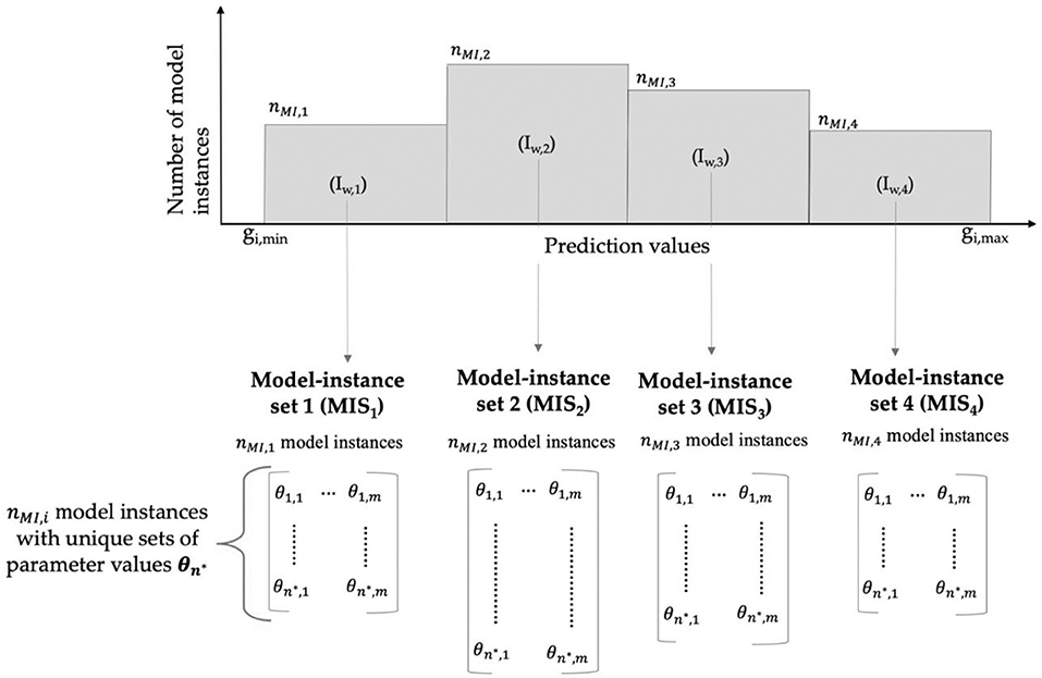
Figure 4. Illustration of the concept of model instance set (MIS) obtained using the hierarchical algorithm (section Sensor-Placement Algorithm—Hierarchical Algorithm).

In LoA 2, the main approximation lies in the reserve capacity calculation for a MIS. The reserve capacity of a MIS_j is taken as the minimum value of RC among instances in the set RC_{min, j} = min(RC_MI,j). Additionally, the probability that a MIS_j is the true CMS is equal to P_j = n_MI,j/n_MI, where n_MI,j is the number of model instances in this MIS. The ${P\left(R{C}^{+}\right)}_{LoA2}$is calculated using the sum of the MIS probability with RC_{min, j} ≥ 1 called $P\left(R{C}_{min}^{+}\right)$. The VoI_EMO is calculated using Equation (17), where N_MIS is the total number of MIS. Additionally, the cost of monitoring is evaluated based on the measurement-system-design framework. As VoI_EMO is an upper bound of the VoI, the monitoring is not justified if VoI_EMO < 0. In case VoI_EMO > 0, a more refined approach is required to evaluate the reserve capacity.

$\begin{array}{ll}Vo{I}_{EMO}={(C_{int}-C_{not})}^{*}{P(R{C}^{+})}_{LoA2}-C_{mon}& (17)\end{array}$

with,

$\begin{array}{ll}{P(R{C}^{+})}_{LoA2}={\displaystyle \sum _j^{N_{MIS}}}{P}_j(R{C}_{min,j}^{+})& (18)\end{array}$

LoA 3—Value of Information With a Probabilistic Approach for Reserve Capacity Assessment (VoI_PA)

In this section, the assessment of the reserve capacity for a population of model instances is further refined by taking into account model uncertainties. In order to assess the reserve capacity of a model instance population, the methodology shown in Figure 5 is adopted from (Proverbio et al., 2018c). For example, serviceability requirements in steel structures imply that the maximum stress in each element is lower than the yield stress. With reference to Figure 5A, stress predictions are computed for each model instance. Then, the total model uncertainty is calculated by combining all source of uncertainties related to the FE model class using the Monte Carlo method (Figure 5B). In Figure 5C, the model uncertainty is added to the discrete distribution of stress predictions and the limit state condition is depicted using a vertical line. In this example, since the entire stress distribution lies below the yield stress, the reserve capacity is assessed by increasing the design load using a load factor LF. Design traffic loads are increased until the probability of failure of the model population equals the target failure probability $p_f^{limitstate}$ defined by design codes. The value of SLS reserve capacity for a specific MIS is equal to the value of load factor LF_set for which the MIS failure probability p_f is equal to $p_f^{limitstate}$. Figure 5D shows the stress distribution at failure. In such situations RC_LF,j = LF_j. The ${P(R{C}^{+})}_{LoA3}$ is calculated using the sum of the MIS probability with LF_j ≥ 1, called $P(R{C}_{LF}^{+})$. Compared to LoA 2, the estimation of ${P(R{C}^{+})}_{LoA3}$ is modified due to the new method for computing the RC of a population of model instances.

FIGURE 5

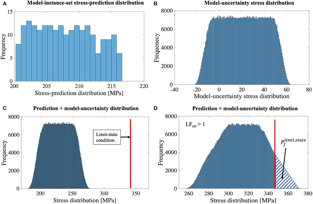
Figure 5. Probabilistic approach for model-instance-population reserve capacity assessment. (A) Model instance population stress prediction; (B) model uncertainty distribution; (C) combination of population and model uncertainty distributions; (D) stress prediction including model uncertainty at failure (load factor LF > 1). The area on the right side of the limit-state condition corresponds to the target failure probability P_f. Original figure based on the concepts of Proverbio et al. (2018c).

Once the reserve capacity of each set of model instances is computed, the VoI_PA is obtained using Equation (19). The VoI_PA is an upper bound of the VoI as, at this stage, it is not reduced by any additional source of uncertainty. When VoI_PA > 0, LoA 4 should be performed. In situations where VoI_PA < 0, monitoring is not recommended.

$\begin{array}{ll}Vo{I}_{PA}={(C_{int}-C_{not})}^{*}{P(R{C}^{+})}_{LoA3}-C_{mon}& (19)\end{array}$

with.

$\begin{array}{ll}{P(R{C}^{+})}_{LoA3}={\displaystyle \sum _j^{N_{MIS}}}{P}_j(R{C}_{LF,j}^{+})& (20)\end{array}$

LoA 4—Value of Information (VoI)

This section discusses the assumption of a perfect information in the VoI estimation. In previous sections, it was assumed that the outcome of the monitoring was exact. However, uncertainties, such as sensor failures may affect field measurements while simplifications often reduce the accuracy of methodologies for sensor placement and structural identification. To evaluate the VoI, each uncertainty source that may affect the estimation of P(RC⁺) has to be evaluated.

Then, all uncertainty sources are combined into the global uncertainty u_tot, which corresponds to the confidence level associated with the VoI estimation. Each uncertainty source u_v is thus defined by a probability distribution having a minimum value u_v,low ≥ 0, and a maximum value u_v,high ≤ 1. Consequently, uncertainty sources can only reduce the VoI estimation as they account probabilistically for the risk of an inaccurate evaluation of P(RC⁺). Equation (21) describes the VoI in probabilistic terms by including the global source of uncertainty u_tot.

$\begin{array}{ll}VoI={(C_{int}-C_{not})}^{*}{P(R{C}^{+})}_{LoA4}-C_{mon}& (21)\end{array}$

with,

$\begin{array}{ll}{{P(R{C}^{+})}_{LoA4}=u}_{tot}^{*}{\displaystyle \sum _j^{N_{MIS}}}{P}_j(R{C}_{LF,j}^{+})& (22)\end{array}$

In order to establish whether monitoring is worthwhile, hypothesis testing is performed (Figure 6). The null hypothesis (i.e., monitoring is worthwhile) adopts a lower bound P_LoA4,low of P(RC⁺), thus minimizing the benefit-cost ratio. The alternative hypothesis (i.e., monitoring is unworthy) adopts an upper bound P_LoA4,high of P(RC⁺), which minimizes the benefit-cost ratio. The upper and lower bounds are fixed at one standard deviation from the mean value of P(RC⁺). When the true benefit-cost ratio lies in this range (dashed area on Figure 6), further investigation is required.

FIGURE 6

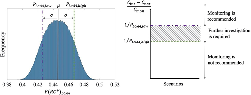
Figure 6. Probabilistic definition of P(RC⁺) and hypothesis testing to justify or reject monitoring.

Parameter Space Sampling Uncertainty

The ${P(R{C}^{+})}_{LoA4}$ estimation is affected by the initial population of model instances. To evaluate the uncertainty related to the model population (u₁), the quality of parameter sampling is investigated. First, each parameter domain r is divided in NP subintervals, for which the corresponding prediction ranges are sufficiently distinct according to engineering judgement. Then, for each subinterval, the observed distribution O and the expected distribution E of samples are compared. A uniform distribution is assumed for the uncertainty u₁, with upper bound equal to 1 and lower bound equal to u_1,low(Equation 23). u_1,low is calculated, similarly to the Pearson's chi-squared test (Pearson, 1900) based on the expected and observed distribution in each parameter domain. When the expected sample distribution and the observed sample distribution are similar, u_1,low approaches 1.

$\begin{array}{ll}{u}_1~Uniform(u_{1,low}=1-{\displaystyle \sum _r^{N_{para}}}\left(\frac{1}{N{P}_{MIS,r}}{\displaystyle \sum _s^{N{P}_{MIS,r}}}\frac{{\left(O_{r,s}-E_{r,s}\right)}^2}{E_{r,s}}\right);1)& (23)\end{array}$

Uncertainty Related to the Expected Information Gain Evaluation

The expected information gain by the measurement system affects the estimation of ${P(R{C}^{+})}_{LoA4}$. Model instances are clustered according to their predictions. At a sensor location i, the initial prediction range — between the smallest prediction g_{i, min} and the largest prediction g_{i, max} — is subdivided into several intervals. The width of each interval is constant and defined based on the combined uncertainty U_i,c (Equation 2). The number of intervals multiplied by the width of each interval is usually larger than the range of model predictions. Since the interval width is fixed, the interval configuration has to be defined. Traditional implementations of the hierarchical algorithm (Papadopoulou et al., 2014; Bertola et al., 2017) selected arbitrary to start intervals on g_i,min.

The selected interval starts influences the assessment of the expected information gain and thus influences the ${P(R{C}^{+})}_{LoA4}$ and eventually the VoI estimation. The uncertainty on the expected information gain is evaluated based on the possible variation of the P(RC⁺), when another choice on the starting point of intervals is made. As no additional information exists, the uncertainty is assumed to have a uniform distribution between a minimum value u_2,low and a maximum value equal to 1 (Equation 24). u_2,low is calculated as the ratio between the evaluations of P(RC⁺), when model-instance the first interval at a sensor location is set on g_i,min and g_i,max, respectively. As the choice in the hierarchical algorithm may either under-estimate or over-estimate P(RC⁺), the lower bound of u_2,low is conservative.

$\begin{array}{ll}{u}_2~Uniform(u_{2,low}=min\left(1;\frac{{\displaystyle {\sum }_l^{N_{MIS}}}{P}_l\left(R{\displaystyle C_{LF,l}^{+}}\right)}{{\displaystyle {\sum }_j^{N_{MIS}}}{P}_j\left(R{\displaystyle C_{LF,j}^{+}}\right)}\right);1)& (24)\end{array}$

Sensor Failure Uncertainty

Bridge load testing requires installing sensor directly on the structure and usually the monitoring is performed during a short period of time. Few sensors may fail, which affects the information gained by the measurement system (Reynders et al., 2013). The uncertainty u₃ assesses the robustness of the information gain to a sensor failure. In this study, the loss of information is evaluated using the variation P(RC⁺) resulting from a sensor failure. In order to determine the magnitude of u₃, the best sensor (i.e., the first sensor selected by the hierarchical algorithm) is assumed to fail and the consequent loss of information is assessed. When the best sensor is removed, P(RC⁺) is equal to $\sum _l^{N_{MIS}^{*}}{P}_l\left(R{C}_l^{+}\right)$. As each sensor is equally likely to fail, the situation in which the best sensor is out of order represents the worst-case scenario. The distribution of uncertainty u₃ is thus assumed to be uniform (Equation 25), and the lower bound u_{3, low} is calculated.

$\begin{array}{ll}{u}_3~Uniform(u_{3,low}=\frac{{\displaystyle {\sum }_l^{N_{MIS}^{*}}}{P}_l(R{C}_l^{+})}{{\sum }_j^{N_{MIS}}{P}_j(R{C}_j^{+})};1)& (25)\end{array}$

Diagnosis Error Uncertainty

Once field measurements are collected, the falsification procedure for model-based diagnosis is performed to determine plausible model instances using a target of reliability (Equation 3). An error in the diagnosis occurs when the correct model is rejected while incorrect models are accepted, leading to wrong conclusions on the parameter identification and then to an inaccurate reserve capacity assessment.

Figure 7 presents the probability of diagnosis error as function of the number of measurements. The probability of a false rejection of the correct model, called type-I error, increases with the number of measurements, while the probability of false acceptance of incorrect models, called type-II error, decreases with the number of measurements. The simultaneous occurrence of type-I and type-II errors is the probability of diagnosis error.

FIGURE 7

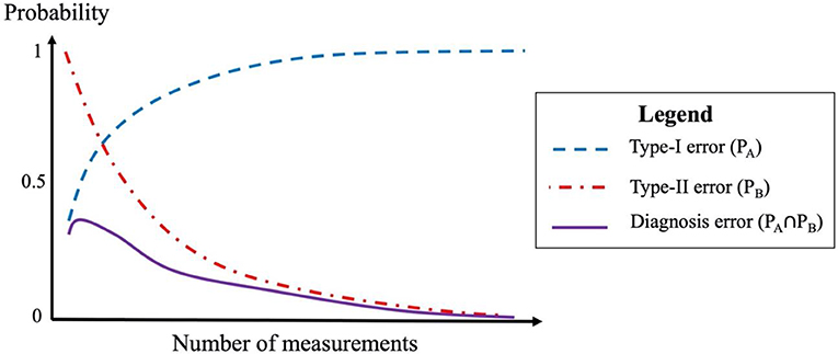
Figure 7. Qualitative example of the probability of diagnosis error as function of number of measurements.

Pasquier et al. (2013) demonstrated that adding new measurements can be beneficial since it improves the robustness of the structural identification to diagnosis error. The sensitivity of the diagnosis error to misevaluation of model uncertainties was investigated. The present study includes a conservative estimation of the probability of diagnosis error P_diag as function of the number of measurements. A similar approach was adopted in Papadopoulou et al. (2016). The uncertainty of diagnosis error is estimated using a uniform distribution (Equation 26). The lower bound u_{4, low} increases when the diagnosis error decreases.

$\begin{array}{ll}{u}_4~Uniform(u_{4,low}=1-P_{diag};1)& (26)\end{array}$

Case Study

The Exeter Bascule Bridge

The Exeter Bascule Bridge (UK) crosses a canal connected to the river Exe. The bridge has a single span of 17.3 m and a total width of about 8.2 m, carrying the traffic and a footway. Built in 1972, the bridge is designed to be lifted to allow the transit of boats. Two longitudinal steel girders are connected to 18 secondary beams. The lightweight deck, consisting of a series of flanked aluminum omega-shaped profiles, is fixed to secondary beams. The South bank edges are simply supported, while the north bank supports are hinges. Two hydraulic jacks, used during lifting operations, are connected to the two longitudinal girders on the north bank side. Figure 8 shows the bridge elevation and a photograph of a static load test. Monitoring devices consist of 11 strain gauges and one precision camera, which is used in combination with a target that is positioned on the bridge. Additionally, five static load configurations can be performed. Consequently, the optimal measurement system is defined by combining 12 potential sensors and five load tests.

FIGURE 8

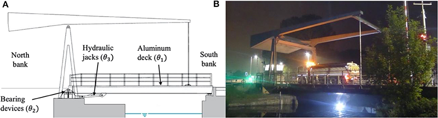
Figure 8. The Exeter Bascule Bridge. (A) Side elevation; (B) photograph of a static load test.

Model Class Selection

Based on a sensitivity analysis at test conditions, three parameters are found to influence the most the structural behavior under this specific loading: the equivalent Young's modulus of the aluminum deck (θ₁), the rotational stiffness of the north bank hinges (θ₂), and the axial stiffness of the hydraulic jacks (θ₃) (Proverbio et al., 2018b). Initial parameter ranges are shown in Table 1. The axial stiffness of hydraulic jacks is used to simulate their contributions as additional load-carrying supports. When the lower bound for θ₃ is used, the two girders are simply supported at the abutments, while the upper bound introduces a semi-rigid support at jack connections.

TABLE 1

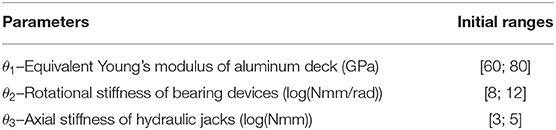
Table 1. Model parameter initial ranges for structural identification.

An initial population of 1,000 model instances is generated using Latin hypercube sampling (McKay et al., 1979). As no additional information is available, parameter ranges are assumed with uniform distributions. The same population is used in order to generate predictions at sensor locations for each load tests. Uncertainties associated with the model class are presented in Table 2. Measurement uncertainties associated with sensor devices are shown in Table 3. They are estimated using manufacturer specifications, conservative engineering judgement, and heuristics. Additional information concerning the model class and uncertainty magnitudes is given in Proverbio et al. (2018a).

TABLE 2

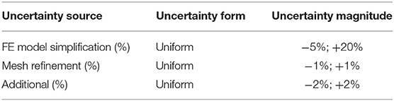
Table 2. Estimation of model-class uncertainties.

TABLE 3

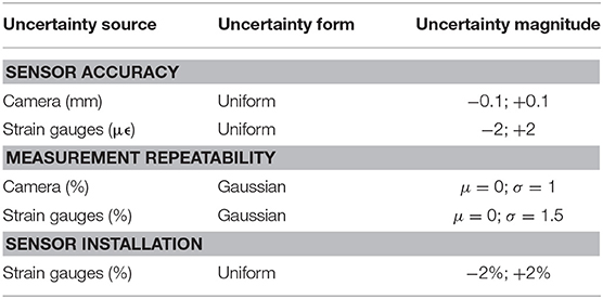
Table 3. Estimation of measurement uncertainties.

Critical Limit States

To evaluate the bridge structural safety, two critical limit states are investigated. Under characteristic design loads, serviceability requirements (SLS) prescribe the maximum Von Mises stress σ_s in each element is lower than the yield strength f_y (Equation 27). The ultimate capacity (ULS) is assessed through the comparison of the maximum bending action M_Ed with its bending capacity M_Rd (Equation 28). Effect of actions are computed under traffic load specifications defined in the current Eurocode EN 1991-2 (EC). Von Mises stress σ_s and bending action M_Ed are computed using the updated model class. When the ultimate capacity is computed, the rotational stiffness of bearing devices is omitted as the support frictional behavior may disappear at high loads. In order to be conservative, the identified values of the rotational stiffness Θ_2,CMS is not taken into account. The lower bound for θ₂ (Table 1) is thus adopted.

$\begin{array}{ll}SLS:{\sigma }_s\left({\Theta }_{1,CMS},{\Theta }_{2,CMS},{\Theta }_{3,CMS}\right)\le f_y& (27)\end{array}$

$\begin{array}{ll}ULS:M_{Ed}\left({\Theta }_{1,CMS},{\Theta }_{3,CMS}\right)\le M_{Rd}=\frac{W_{pl}·f_y}{{\gamma }_{M0}}& (28)\end{array}$

Preliminary Reserve Capacity Assessments

In this section, preliminary assessments of reserve capacity are calculated. The aim is to determine if the information collected during monitoring may influence the structural assessment. Values of reserve capacity computed using Θ_cons and Θ_opt are presented in Table 4. For both limit states, results show that RC(Θ_cons,LS) < 1 and RC(Θ_opt,LS) > 1, thus meeting the two conditions for preliminary assessment. Consequently, the VoI is estimated as described in the following sections.

TABLE 4

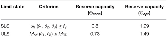
Table 4. Preliminary reserve capacity assessments for serveacibility (SLS) and ultimate (ULS) limit states.

LoA 1—VoI_PMO

In this section, the LoA1 for VoI estimation is presented. Model instances belonging to the population generated are used to obtain individual predictions of reserve capacity for both limit states. Figure 9 shows reserve capacity distributions of model instances. For both limit states, the reserve capacity distribution presents a first peak with a RC < 1 and a lower second peak when RC > 1. Therefore, possible reserve capacity ranges are significantly influenced by the values of model parameters. The monitoring output, based on true measurements, may lead to conclusions that the bridge presents reserve capacity or requires interventions. Estimating the VoI supports asset managers with quantitative information on the potential of bridge monitoring. Additionally, the distribution spread is larger for SLS (Figure 9A) than for ULS (Figure 9B), showing that model-parameter values have greater influence on the SLS assessment.

FIGURE 9

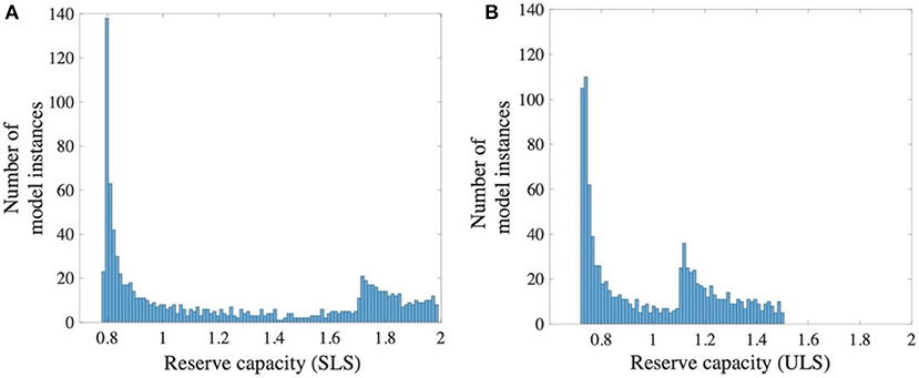
Figure 9. Model-instance reserve capacity distributions. (A) SLS; (B) ULS.

${P(R{C}^{+})}_{LoA1}$ is defined as the ratio between the number of model instances with RC ≥ 1 N_MI(RC⁺) over the total number of model instances N_MI. The evaluation of VoPI_PMO requires computing the costs for the two scenarios (C_int and C_not) and monitoring cost C_mon, which allow defining the minimum benefit-cost ratio that justifies monitoring. Table 5 reports values of ${P(R{C}^{+})}_{LoA1}$ and the minimum benefit-cost ratio for both SLS and ULS. Minimum benefit-cost ratios are smaller for SLS than for ULS, as the number of model instances with a reserve capacity is larger for SLS. Based on true benefit-cost ratio, asset managers can decide whether to proceed with the interventions or to perform the LoA 2.

TABLE 5

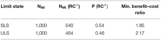
Table 5. Evaluation of the minimum benefit-cost ratio between cost savings C_int−C_not and cost of monitoring C_mon to justify monitoring—LoA 1.

LoA 2—VoI_EMO

In this section, the expected information gain from the measurement system is used to provide more accurate estimations of VoI, according to the framework presented in section Sensor-Placement Algorithm—Hierarchical Algorithm. Following Bertola et al. (2019), the recommended measurement system depends on asset manager preferences. Three scenarios are introduced: low-cost monitoring, equal weight scenario, and maximization of information gain. Recommended measurement systems are presented in Figure 10. These scenarios were obtained taking into account five performance criteria: information gain, monitoring costs, sensor installation, robustness of information gain to sensor failure, and ability to detect outliers. As explained in Bertola et al. (2019), sensor locations close to the hydraulic jack are preferred as this parameter has significant influence on model predictions.

FIGURE 10

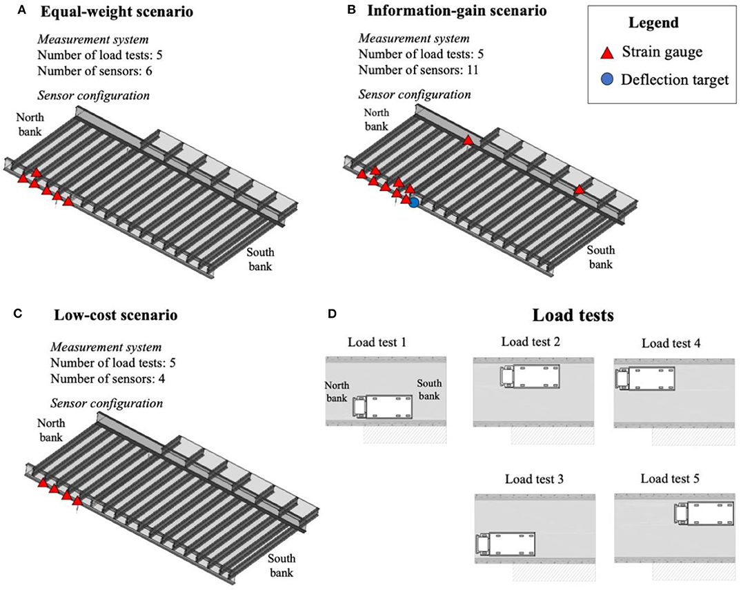
Figure 10. Recommended measurement system as function of asset manager preferences. (A) Equal-weight scenario; (B) Maximization of information-gain scenario; (C) Low-cost scenario. (D) Load tests. Original figure based on the concepts of Bertola et al. (2019).

Table 6 presents characteristics of measurement-system scenarios. Measurement systems differ by the number of sensors (N_sens) installed on the bridge. However, they all involve five load tests (N_loadtest) and thus differ in the number of measurements N_meas, calculated as the multiplication of the number of sensors and the number of load tests. The information gain and the cost of monitoring increase with the number of measurements, showing the conflicting nature of performance criteria. Similarly, the number of MISs (N_MIS) increases significantly with the number of measurements. This result shows that adding more measurements helps discriminate between model instances, thus resulting in a smaller CMS after monitoring. However, this information comes at an additional cost. Therefore, a more precise reserve capacity assessment may not be justified by its benefits in influencing asset manager decisions.

TABLE 6

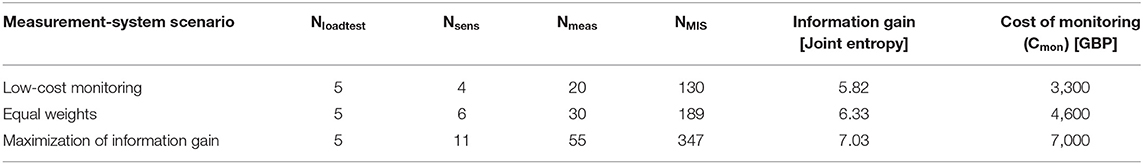
Table 6. Characteristics of monitoring scenarios.

Figure 11 presents RC distributions of MIS for both SLS and ULS using the expected information gain from two monitoring scenarios: low-cost monitoring (Figures 11A,B) and maximization of information gain (Figures 11C,D). For both scenarios, SLS and ULS distributions are similar with the largest likelihood of reserve capacity around RC ≈ 0.8 for SLS and RC ≈ 0.7 for ULS. The SLS reserve capacity range is slightly larger than the ULS range, showing that parameter values influence more the SLS assessment. When comparing measurement system scenarios, reserve capacity distributions are modified, showing that increasing the number of measurements leads to more precise assessments of the expected reserve capacity. Nevertheless, as reserve capacity ranges are large, it may not increase significantly P(RC⁺).

FIGURE 11

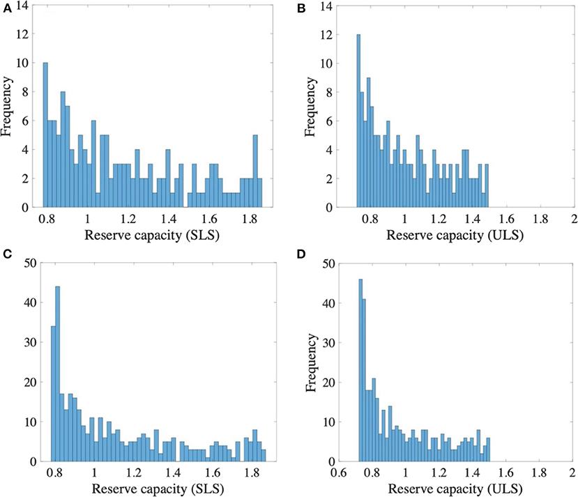
Figure 11. Reserve capacity distributions of model instance-sets using the minimum value of RC in each model instance set (MIS). (A) Low-cost monitoring scenario—SLS; (B) low-cost monitoring scenario—ULS; (C) scenario of maximization of information gain—SLS; (D) scenario of maximization of information gain—ULS.

Table 7 shows values of the minimum benefit-cost ratio to justify monitoring for alternative measurement system scenarios at LoA 2. Results are similar to LoA 1 (Table 5) due to the particular reserve capacity distributions of the initial model instance set (Figure 9). For both limit states, the scenario of maximization of information gain has the largest ${P(R{C}^{+})}_{LoA2}$, showing that increasing the number of measurements increases the probability to find reserve capacity. However, minimum cost savings to justify monitoring are smaller for the low-cost monitoring scenario. This result shows that a more expensive measurement system may not be justified by its effects on asset manager decision. The next section investigates this option by improving the VoI estimation.

TABLE 7

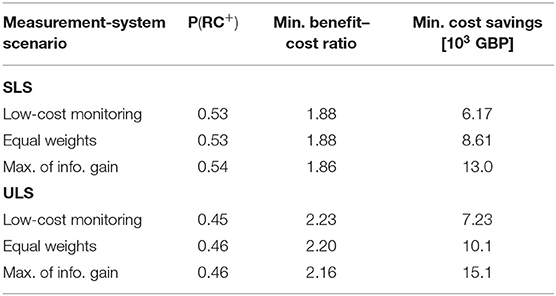
Table 7. Evaluation of the minimum benefit–cost ratio between cost savings C_int−C_not and cost of monitoring C_mon to justify monitoring—LoA 2.

LoA 3—VoI_PA

In this section, the reserve capacity of MIS is assessed by means of a probabilistic approach. First, model class uncertainties are included to predictions of steel stress (SLS) and bending moment (ULS). Then, design loads are progressively increased until the prediction distribution reaches a target of probability of failure, fixed at $P_f^{SLS}=10^{-1}$ for SLS and $P_f^{ULS}=10^{-4}$ for ULS, respectively (Proverbio et al., 2018c).

Figure 12 presents new reserve capacity distributions for both limit states for two measurement system scenarios: low-cost monitoring (Figures 12A,B) and maximization of information gain (Figures 12C,D). Reserve capacity distributions are significantly influenced by the measurement-system scenario. More measurements lead to more precise assessments of the expected reserve capacity. When compared with previous reserve capacity distributions (Figure 11), new distributions exhibit similar shapes. However, reserve capacity values are smaller due to the presence of model uncertainties.

FIGURE 12

Figure 12. Reserve capacity distributions of model instance-sets using the population-based probabilistic approach for RC estimation of MIS. (A) low-cost monitoring scenario—SLS; (B) low-cost monitoring scenario—ULS; (C) scenario of maximization of information gain—SLS; (D) scenario of maximization of information gain—ULS.

For each measurement-system scenario, Table 8 presents evaluations of the minimum benefit-cost ratio to justify monitoring at LoA 3. The ${P\left(R{C}^{+}\right)}_{LoA3}$estimations are similar for all measurement systems. Consequently, the scenario of low-cost monitoring shows the smallest cost savings to justify the monitoring. When compared to LoA 2 (Table 7), minimum benefit-cost ratios are larger as reserve capacity estimations decrease when model uncertainties are taken into account. Additional uncertainties related to the monitoring outcome are introduced in the next section.

TABLE 8

Table 8. Evaluation of the minimum benefit–cost ratio between cost savings C_int−C_not and cost of monitoring C_mon to justify monitoring—LoA 3.

LoA 4—VoI

Monitoring uncertainty sources are evaluated for each measurement-system scenario. Uncertainty sources u_i are chosen as uniform distribution bounded between u_v,low and 1. Results are presented in Table 9.

TABLE 9

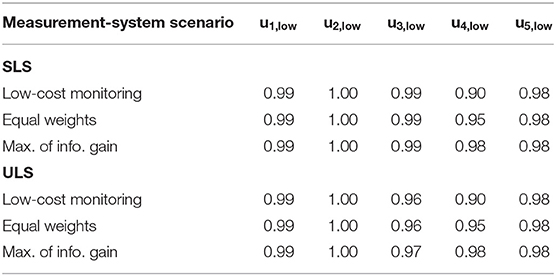
Table 9. Uncertainty evaluations of monitoring scenarios.

The first source of uncertainty u₁ is related to the quality of the sampling used. In this study, 1,000 model instances are generated using LHS for a three-parameter space. Due to the sampling technic used and the number of model instances, parameter distributions are almost uniform (expected distribution). Additionally, u₁ is independent of the measurement-system scenarios.

The accuracy of sensor placement algorithm is evaluated in the second uncertainty source u₂. P(RC⁺) estimations are evaluated for a range of interval starting points, for each measurement system scenario. Results show that the hypothesis to start intervals at minimum values of predictions is conservative and decreases P(RC⁺) estimations by 1–2%. This uncertainty source does thus not affect the VoI estimation.

The uncertainty source u₃ accounts for possible sensor failure(s). The best sensor is assumed to fail and its expected information gain is removed. For each measurement system scenario and limit state, u_{3, low} is calculated using Equation (25).

The risk of diagnosis error, which is function of the number of measurements, is estimated using the uncertainty source u₄. As this uncertainty is related to system identification, the selected critical limit state does not affect u₄. Following a conservative hypothesis of maximum misevaluation of model uncertainties of 100% (Pasquier et al., 2013; Papadopoulou et al., 2016), the probability of diagnosis error is estimated to be 10, 5, and 2% for 20, 30, and 55 field measurements, respectively. u₄ is then calculated using Equation (26).

An additional uncertainty is added to cover potential remaining uncertainty sources. Based on engineering judgment, the additional uncertainty u₅ is taken as a uniform distribution bounded between u_{5, low} equal to 0.98 and 1. Once each uncertainty source is estimated, the global uncertainty u_tot is computed and hypothesis testing is conducted.

Table 10 shows, for each scenario, the minimum benefit-cost ratios to justify monitoring, while Table 11 shows the maximum benefit-cost ratios to avoid monitoring. As small uncertainties are present (Table 9), upper and lower bounds of benefit-cost ratio are similar. For the same measurement system, minimum cost savings are similar to those reported in Table 8. For both limit states, the measurement system scenario of low-cost monitoring presents the smallest minimum cost savings to justify testing the bridge. Minimum costs savings are much larger for ULS than SLS as P(RC⁺) evaluations are much lower for ULS. This result shows that the parameter identification using monitoring is unlikely to influence RC assessment for ULS. Cost savings must be significantly larger to justify monitoring for ULS.

TABLE 10

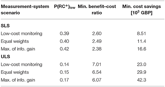
Table 10. Evaluation of the minimum benefit–cost ratio between cost savings C_int−C_not and cost of monitoring C_mon to justify monitoring—LoA 4.

TABLE 11

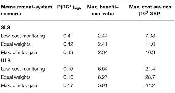
Table 11. Evaluation of the maximum benefit–cost ratio between cost savings C_int−C_not and cost of monitoring C_mon to avoid monitoring—LoA 4.

Figure 13 presents the thresholds of the benefit-cost ratio for each monitoring scenario, which differ by the number of measurements, and both limit states. This figure provides a visualization of results in Tables 10, 11. The dashed areas refer to non-informative values of benefit-cost ratios, for which further investigation is required. When the number of measurements increases, global uncertainties are reduced and thus the two thresholds are closer. This result shows that additional measurements reduce uncertainties on monitoring outcomes. Nevertheless, adding measurements does not significantly improve the minimum benefit-cost ratio to justify monitoring for SLS and may not be justified by the associated increase of monitoring costs. A comparison of monitoring outcomes is presented below.

FIGURE 13

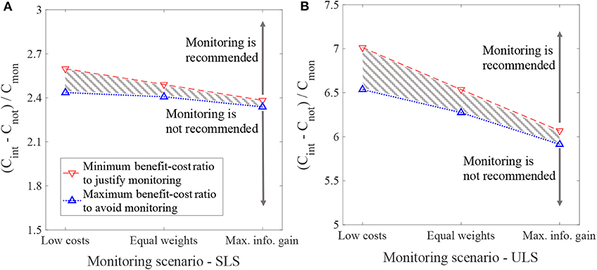
Figure 13. Benefit–cost ratios to justify or reject monitoring for each monitoring scenario. (A) SLS; (B) ULS.

Measurement System Comparison

In this section, the measurement system scenarios are compared using minimum benefit-cost ratio and minimum cost savings to justify monitoring. The aim is to determine which measurement system should be recommended to asset managers, according to its VoI.

For each measurement system scenario, Figure 14A shows the minimum benefit-cost ratio as function of the level of approximation for SLS. Figure 14B shows the minimum cost savings to justify monitoring the bridge. For the estimation of VoI (LoA 4), only the assumption that testing the bridge is unworthy (upper bound of minimum cost savings) is presented (Figure 13). In both cases, the minimum cost savings increases with the LoA, showing the upper bound VoI estimations of the framework, which correspond to lower bound estimations of minimum benefit-cost ratios (Table 10). The scenario of maximization of information gain provides the smallest minimum benefit-cost ratio to justify monitoring. However, the scenario of low-cost monitoring presents the smallest minimum cost savings to justify the bridge load testing and, therefore, it is recommended for SLS. Figures 14C,D present minimum benefit-cost ratios and cost savings to justify monitoring for ULS with similar observations when compared to SLS. The main difference between SLS and ULS is that ULS requires much larger cost savings to justify monitoring.

FIGURE 14

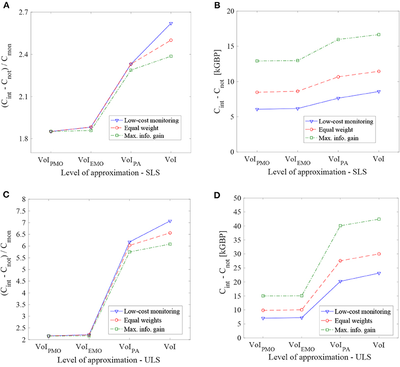
Figure 14. Minimum benefit–cost ratios $\frac{C_{int}-C_{not}}{C_{mon}}$ and cost savings C_int−C_not to justify monitoring as function of the level of approximation. (A) Benefit–cost ratio—SLS; (B) including C_mon evaluation—SLS; (C) benefit–cost ratio—ULS; (D) including C_mon evaluation—ULS.

For both limit states, the low-cost scenario is therefore recommended as it presents the smallest minimum cost savings to justify monitoring. This conclusion differs from the results of the recommended measurement system based on MCDA analysis (Table 6), where the information gain is observed to increase with the number of measurements. The information gain is measured using the joint entropy, which takes into account only the identifiability of model instances. On the contrary, the VoI takes into account the influence of parameter identifiability on reserve capacity assessment. As the VoI estimation requires significantly larger computational time, using a MCDA methodology to reduce the set of possible measurement systems is suggested. Nevertheless, the VoI estimation is recommended when the goal is to select the appropriate measurement system among a set of good alternatives.

Discussion

The following limitations of the work are recognized: the success of any model-based methodology for sensor placement or VoI estimation depends on the quality of the numerical behavior model used to compute predictions. The reliability of model assumptions, such as model-class definition, should be verified via visual inspection. In case a wrong model class is selected, with EDMF, all model instances are typically falsified, thus suggesting a revision of the initial assumptions. This risk was not taken into account in the present study as it still provides useful information to asset managers. When a model class is rejected, the information gained by the monitoring still leads to better understanding of the structural behavior and this understanding helps avoid further wrong assessment of the reserve capacity. In such situations, monitoring remains useful.

In the present study, the ultimate limit state of the case study involves only evaluations at first yield of steel. For case studies requiring NFLEA simulations, such as reinforced concrete bridges, the estimation of uncertainties in non-linear analysis is challenging. Additionally, these uncertainties cannot be significantly reduced using elastic measurements. Before performing reserve capacity assessment, model validation is recommended (Cervenka, 2013). VoI evaluations for static load testing might be inappropriate. Additionally, computing the VoI requires the evaluation of the reserve capacity for a large number of model instance sets and thus may be computationally expensive. Authors thus suggest to limit the scope of the proposed framework to serviceability limit states and ultimate limit states involving evaluation only at first yield, such as for the case study described in this paper.

The parameters that can be identified during static load testing are mostly related to the structural stiffness and boundary conditions. Often these parameters do not dictate the ultimate carrying capacity as they provide little information on the material strength and material non-linear behavior. Future work will involve the use of non-destructive tests to update relevant parameters at ULS.

The estimation of P(RC⁺) is influenced by the initial assumptions of model-parameter distributions. In the Exeter Bascule Bridge, the three model parameters are assumed having uniform distributions between bounds of parameter values, where parameter bounds represent lowest and largest plausible values. These choices were made based on engineering judgement and visual inspection. Wrong initial hypotheses on model parameter distributions may lead to an inaccurate estimation of P(RC⁺).

The VoI estimation of monitoring scenarios also depends on the possible decisions of asset managers. In the present study, only two actions are considered, depending of the bridge reserve capacity. Intervention costs C_imp and do-nothing costs C_not are assumed not to be dependent on the reserve capacity assessment. In the present study, only economic costs are taken into account. Total costs may also include social costs calculated for example as the total travel time delay during interventions, environmental costs of the structural improvement and a lifecycle cost of the “do-nothing” scenarios. These cost refinements may influence the decision on whether the bridge should be monitored.

Conclusions

Efficient asset management of existing civil infrastructure is necessary. This paper contains a proposal for a framework to estimate the value of information (VoI) of bridge load testing for reserve capacity assessment based on the EDMF methodology. Conclusions are as follows:

• The framework provides useful guidance to asset managers to evaluate whether the information from monitoring influences the assessment of reserve capacity, particularly when the critical limit state is either serviceability or ultimate when first yield is a good approximation.

• The approach, using levels of approximation, helps reveal if more accurate estimation of VoI is needed, thus reducing unnecessary complex analyses when controlled-condition monitoring would not provide sufficient information to influence asset-manager actions.

• A full-scale case study demonstrates that the framework supports asset managers in the choice of the optimal measurement system when multiple monitoring scenarios are proposed.

Future work involves comparing the effects of intervention actions, such as load testing and non-destructive tests on the reserve capacity assessment.

Data Availability Statement

The original contributions presented in the study are included in the article, further inquiries can be directed to the corresponding author.

Author Contributions

NB elaborated the methodologies for measurement-system design and value of information. MP assisted in the elaboration of the case study and reserve capacity assessment. IS was actively involved in developing and adapting the data interpretation methodology for the present study. All authors reviewed and accepted the final version.

Funding

The research was conducted at the Future Cities Laboratory at the Singapore-ETH Centre, which was established collaboratively between ETH Zurich and Singapore's National Research Foundation (FI 370074011) under its Campus for Research Excellence and Technological Enterprise program.

Conflict of Interest

MP was employed by the company COWI A/S.

The remaining authors declare that the research was conducted in the absence of any commercial or financial relationships that could be construed as a potential conflict of interest.

Acknowledgments

The authors gratefully acknowledge the University of Exeter (J. Brownjohn, P. Kripakaran, and the Full Scale Dynamics Ltd. [UK]) for support during load tests in the scope of the case study and M. Pozzi (CMU) for the valuable input.

References

Argyris, C., Papadimitriou, C., and Panetsos, P. (2017). Bayesian optimal sensor placement for modal identification of civil infrastructures. J. Smart Cities 2:69–86. doi: 10.18063/JSC.2016.02.001

CrossRef Full Text | Google Scholar

Beck, J. L., and Katafygiotis, L. S. (1998). Updating models and their uncertainties. I: Bayesian statistical framework. J. Eng. Mech. 124, 455–461. doi: 10.1061/(ASCE)0733-9399(1998)124:4(455)

CrossRef Full Text | Google Scholar

Behmanesh, I., Moaveni, B., Lombaert, G., and Papadimitriou, C. (2015). Hierarchical Bayesian model updating for structural identification. Mech. Syst. Signal Process. 64–65, 360–376. doi: 10.1016/j.ymssp.2015.03.026

CrossRef Full Text | Google Scholar

Bertola, N. J., Cinelli, M., Casset, S., Corrente, S., and Smith, I. F. C. (2019). A multi-criteria decision framework to support measurement-system design for bridge load testing. Adv. Eng. Inform. 39, 186–202. doi: 10.1016/j.aei.2019.01.004

CrossRef Full Text | Google Scholar

Bertola, N. J., Papadopoulou, M., Vernay, D. G., and Smith, I. F. C. (2017). Optimal multi-type sensor placement for structural identification by static-load testing. Sensors 17:2904. doi: 10.3390/s17122904

PubMed Abstract | CrossRef Full Text | Google Scholar

Bertola, N. J., and Smith, I. F. C. (2019). A methodology for measurement-system design combining information from static and dynamic excitations for bridge load testing. J. Sound Vib. 463:114953. doi: 10.1016/j.jsv.2019.114953

CrossRef Full Text | Google Scholar

Brownjohn, J. M. W., De Stefano, A., Xu, Y.-L., Wenzel, H., and Aktan, A. E. (2011). Vibration-based monitoring of civil infrastructure: challenges and successes. J. Civil Struct. Health Monit. 1, 79–95. doi: 10.1007/s13349-011-0009-5

CrossRef Full Text | Google Scholar

Brynjarsdóttir, J., and O'Hagan, A. (2014). Learning about physical parameters: the importance of model discrepancy. Inv. Probl. 30:114007. doi: 10.1088/0266-5611/30/11/114007

CrossRef Full Text | Google Scholar

Catbas, F., Kijewski-Correa, T., Lynn, T., and Aktan, A. (2013). Structural Identification of Constructed Systems. Reston, VA: American Society of Civil Engineers.

Google Scholar

Cervenka, V. (2013). Reliability-based non-linear analysis according to fib Model Code 2010. Struct. Concrete 14, 19–28. doi: 10.1002/suco.201200022

CrossRef Full Text | Google Scholar

Cervenka, V., Cervenka, J., and Kadlec, L. (2018). Model uncertainties in numerical simulations of reinforced concrete structures. Struct. Concrete 19, 2004–2016. doi: 10.1002/suco.201700287

CrossRef Full Text | Google Scholar

Corrente, S., Figueira, J. R., and Greco, S. (2014). The SMAA-PROMETHEE method. Eur. J. Oper. Res. 239, 514–522. doi: 10.1016/j.ejor.2014.05.026

CrossRef Full Text | Google Scholar

Dubbs, N., and Moon, F. (2015). Comparison and implementation of multiple model structural identification methods. J. Struct. Eng. 141:04015042. doi: 10.1061/(ASCE)ST.1943-541X.0001284

PubMed Abstract | CrossRef Full Text | Google Scholar

Ellis, H., Jiang, M., and Corotis, R. B. (1995). Inspection, maintenance, and repair with partial observability. J. Infrastruct. Syst. 1, 92–99. doi: 10.1061/(ASCE)1076-0342(1995)1:2(92)

CrossRef Full Text | Google Scholar

Fereshtehnejad, E., and Shafieezadeh, A. (2017). A randomized point-based value iteration POMDP enhanced with a counting process technique for optimal management of multi-state multi-element systems. Struct. Saf. 65, 113–125. doi: 10.1016/j.strusafe.2017.01.003

CrossRef Full Text | Google Scholar

Goulet, J.-A., Der Kiureghian, A., and Li, B. (2015). Pre-posterior optimization of sequence of measurement and intervention actions under structural reliability constraint. Struct. Saf. 52, 1–9. doi: 10.1016/j.strusafe.2014.08.001

CrossRef Full Text | Google Scholar

Goulet, J.-A., Kripakaran, P., and Smith, I. F. C. (2010). Multimodel structural performance monitoring. J. Struct. Eng. 136, 1309–1318. doi: 10.1061/(ASCE)ST.1943-541X.0000232

CrossRef Full Text | Google Scholar

Goulet, J.-A., and Smith, I. F. C. (2012). Predicting the usefulness of monitoring for identifying the behavior of structures. J. Struct. Eng. 139, 1716–1727. doi: 10.1061/(ASCE)ST.1943-541X.0000577

CrossRef Full Text | Google Scholar

Goulet, J.-A., and Smith, I. F. C. (2013). Structural identification with systematic errors and unknown uncertainty dependencies. Comput. Struct. 128, 251–258. doi: 10.1016/j.compstruc.2013.07.009

CrossRef Full Text | Google Scholar

Hendy, C. R., Man, L. S., Mitchell, R. P., and Takano, H. (2016). “Reduced partial factors for assessment in UK assessment standards,” in Maintenance, Monitoring, Safety, Risk and Resilience of Bridges and Bridge Networks, eds T. N. Bittencourt, D. Frangopol, and A. Beck (Leiden: CRC press), 405.

Google Scholar

Heredia-Zavoni, E., and Esteva, L. (1998). Optimal instrumentation of uncertain structural systems subject to earthquake ground motions. Earthq. Eng. Struct. Dyn. 27, 343–362. doi: 10.1002/(SICI)1096-9845(199804)27:4<343::AID-EQE726>3.0.CO;2-F

CrossRef Full Text | Google Scholar

Kammer, D. C. (2005). Sensor set expansion for modal vibration testing. Mech. Syst. Signal Process. 19, 700–713. doi: 10.1016/j.ymssp.2004.06.003

CrossRef Full Text | Google Scholar

Katafygiotis, L. S., and Beck, J. L. (1998). Updating models and their uncertainties. II: model identifiability. J. Eng. Mech. 124, 463–467. doi: 10.1061/(ASCE)0733-9399(1998)124:4(463)

CrossRef Full Text | Google Scholar

Lam, H.-F., Yang, J., and Au, S.-K. (2015). Bayesian model updating of a coupled-slab system using field test data utilizing an enhanced Markov chain Monte Carlo simulation algorithm. Eng. Struct. 102, 144–155. doi: 10.1016/j.engstruct.2015.08.005

CrossRef Full Text | Google Scholar

Li, S., and Pozzi, M. (2019). What makes long-term monitoring convenient? A parametric analysis of value of information in infrastructure maintenance. Struct. Control Health Monit. 26:e2329. doi: 10.1002/stc.2329

CrossRef Full Text | Google Scholar

Li, W., Chen, S., Jiang, Z., Apley, D. W., Lu, Z., and Chen, W. (2016). Integrating bayesian calibration, bias correction, and machine learning for the 2014 sandia verification and validation challenge problem. J. Verif. Valid. Uncert. 1:011004. doi: 10.1115/1.4031983

CrossRef Full Text | Google Scholar

Luque, J., and Straub, D. (2016). Reliability analysis and updating of deteriorating systems with dynamic Bayesian networks. Struct. Saf. 62, 34–46. doi: 10.1016/j.strusafe.2016.03.004

CrossRef Full Text | Google Scholar

Malings, C., and Pozzi, M. (2016a). Conditional entropy and value of information metrics for optimal sensing in infrastructure systems. Struct. Saf. 60, 77–90. doi: 10.1016/j.strusafe.2015.10.003

CrossRef Full Text | Google Scholar

Malings, C., and Pozzi, M. (2016b). Value of information for spatially distributed systems: application to sensor placement. Reliabil. Eng. Syst. Saf. 154, 219–233. doi: 10.1016/j.ress.2016.05.010

CrossRef Full Text | Google Scholar

Malings, C., and Pozzi, M. (2019). Submodularity issues in value-of-information-based sensor placement. Reliabil. Eng. Syst. Saf. 183, 93–103. doi: 10.1016/j.ress.2018.11.010

CrossRef Full Text | Google Scholar

McKay, M. D., Beckman, R. J., and Conover, W. J. (1979). Comparison of three methods for selecting values of input variables in the analysis of output from a computer code. Technometrics 21, 239–245. doi: 10.1080/00401706.1979.10489755

CrossRef Full Text | Google Scholar

Miller, R. A., Aktan, A. E., and Shahrooz, B. M. (1994). Destructive testing of decommissioned concrete slab bridge. J. Struct. Eng. 120, 2176–2198. doi: 10.1061/(ASCE)0733-9445(1994)120:7(2176)

CrossRef Full Text | Google Scholar

Muttoni, A., and Ruiz, M. F. (2012). Levels-of-a pproximation approach in codes of practice. Struct. Eng. Int. 22, 190–194. doi: 10.2749/101686612X13291382990688

CrossRef Full Text | Google Scholar

Pai, S. G. S., Nussbaumer, A., and Smith, I. F. C. (2018). Comparing structural identification methodologies for fatigue life prediction of a highway bridge. Front. Built Environ. 3:73. doi: 10.3389/fbuil.2017.00073

CrossRef Full Text | Google Scholar

Papadimitriou, C. (2004). Optimal sensor placement methodology for parametric identification of structural systems. J. Sound Vib. 278, 923–947. doi: 10.1016/j.jsv.2003.10.063

CrossRef Full Text | Google Scholar

Papadimitriou, C., Beck, J. L., and Au, S.-K. (2000). Entropy-based optimal sensor location for structural model updating. J. Vib. Control 6, 781–800. doi: 10.1177/107754630000600508

CrossRef Full Text | Google Scholar

Papadimitriou, C., and Lombaert, G. (2012). The effect of prediction error correlation on optimal sensor placement in structural dynamics. Mech. Syst. Signal Process. 28, 105–127. doi: 10.1016/j.ymssp.2011.05.019

CrossRef Full Text | Google Scholar

Papadopoulou, M., Raphael, B., Smith, I. F. C., and Sekhar, C. (2014). Hierarchical sensor placement using joint entropy and the effect of modeling error. Entropy 16, 5078–5101. doi: 10.3390/e16095078

CrossRef Full Text | Google Scholar

Papadopoulou, M., Raphael, B., Smith, I. F. C., and Sekhar, C. (2016). Evaluating predictive performance of sensor configurations in wind studies around buildings. Adv. Eng. Inform. 30, 127–142. doi: 10.1016/j.aei.2016.02.004

CrossRef Full Text | Google Scholar

Papakonstantinou, K. G., and Shinozuka, M. (2014a). Planning structural inspection and maintenance policies via dynamic programming and Markov processes. Part I: theory. Reliabil. Eng. Syst. Saf. 130, 202–213. doi: 10.1016/j.ress.2014.04.005

CrossRef Full Text | Google Scholar

Papakonstantinou, K. G., and Shinozuka, M. (2014b). Planning structural inspection and maintenance policies via dynamic programming and Markov processes. Part II: POMDP implementation. Reliabil. Eng. Syst. Saf. 130, 214–224. doi: 10.1016/j.ress.2014.04.006

CrossRef Full Text | Google Scholar

Pasquier, R., Goulet, J.-A., Acevedo, C., and Smith, I. F. C. (2014). Improving fatigue evaluations of structures using in-service behavior measurement data. J. Bridge Eng. 19:04014045. doi: 10.1061/(ASCE)BE.1943-5592.0000619

CrossRef Full Text | Google Scholar

Pasquier, R., Goulet, J.-A., and Smith, I. F. C. (2013). “Model-based data interpretation and diagnosis robustness,” in Safety, Reliability, Risk and Life-Cycle Performance of Structures & Infrastructures, eds G. Deodatis, B. R. Ellingwood, and D. M. Frangopol (New York, NY: Taylor & Francis Group), 2497–2504. doi: 10.1201/b16387-361

CrossRef Full Text | Google Scholar

Pasquier, R., Goulet, J.-A., and Smith, I. F. C. (2017). Measurement system design for civil infrastructure using expected utility. Adv. Eng. Inform. 32, 40–51. doi: 10.1016/j.aei.2016.12.002

CrossRef Full Text | Google Scholar

Pasquier, R., and Smith, I. F. C. (2015). Robust system identification and model predictions in the presence of systematic uncertainty. Adv. Eng. Inform. 29, 1096–1109. doi: 10.1016/j.aei.2015.07.007

CrossRef Full Text | Google Scholar

Pasquier, R., and Smith, I. F. C. (2016). Iterative structural identification framework for evaluation of existing structures. Eng. Struct. 106, 179–194. doi: 10.1016/j.engstruct.2015.09.039

CrossRef Full Text | Google Scholar

Pearson, K. F. R. S. (1900). X. On the criterion that a given system of deviations from the probable in the case of a correlated system of variables is such that it can be reasonably supposed to have arisen from random sampling AU–Pearson, Karl. Lond. Edinb. Dublin Philos. Mag. J. Sci. 50, 157–175. doi: 10.1080/14786440009463897

CrossRef Full Text | Google Scholar

Pimentel, M., Brüwhiler, E., and Figueiras, J. (2010). Extended cracked membrane model for the analysis of RC panels. Eng. Struct. 32, 1964–1975. doi: 10.1016/j.engstruct.2010.02.030

CrossRef Full Text | Google Scholar

Pozzi, M., Zonta, D., Wang, W., and Chen, G. (2010). “A framework for evaluating the impact of structural health monitoring on bridge management,” in Bridge Maintenance, Safety, Management and Life-Cycle Optimization–Proceedings of the 5th International Conference on Bridge Maintenance, Safety and Management (Philadelphia, PA: CRC Press), 161–162. doi: 10.1201/b10430-91

CrossRef Full Text | Google Scholar

Proverbio, M., Bertola, N. J., and Smith, I. F. C. (2018a). Outlier-detection methodology for structural identification using sparse static measurements. Sensors 18:1702. doi: 10.3390/s18061702

PubMed Abstract | CrossRef Full Text | Google Scholar

Proverbio, M., Costa, A., and Smith, I. F. C. (2018b). Sensor data interpretation with clustering for interactive asset-management of urban systems. J. Comput. Civil Eng. 32:04018050. doi: 10.1061/(ASCE)CP.1943-5487.0000793

CrossRef Full Text | Google Scholar

Proverbio, M., Vernay, D. G., and Smith, I. F. C. (2018c). Population-based structural identification for reserve capacity assessment of existing bridges. J. Civil Struct. Health Monit. 8, 363–382. doi: 10.1007/s13349-018-0283-6

PubMed Abstract | CrossRef Full Text | Google Scholar

Raiffa, H., and Schlaifer, R. (1961). Applied Statistical Decision Theory. Boston, MA: Division of Research, Harvard University.

Google Scholar

Reynders, E., Wursten, G., and De Roeck, G. (2013). Output-only structural health monitoring in changing environmental conditions by means of nonlinear system identification. Struct. Health Monit. 13, 82–93. doi: 10.1177/1475921713502836

CrossRef Full Text | Google Scholar

Richard, B., Epaillard, S., Cremona, C., Elfgren, L., and Adelaide, L. (2010). Nonlinear finite element analysis of a 50 years old reinforced concrete trough bridge. Eng. Struct. 32, 3899–3910. doi: 10.1016/j.engstruct.2010.09.003

CrossRef Full Text | Google Scholar

Robert-Nicoud, Y., Raphael, B., Burdet, O., and Smith, I. F. C. (2005c). Model identification of bridges using measurement data. Comput. Aided Civil Infrastruct. Eng. 20, 118–131. doi: 10.1111/j.1467-8667.2005.00381.x

CrossRef Full Text

Robert-Nicoud, Y., Raphael, B., and Smith, I. F. C. (2005a). Configuration of measurement systems using Shannon's entropy function. Comput. Struct. 83, 599–612. doi: 10.1016/j.compstruc.2004.11.007

CrossRef Full Text | Google Scholar

Robert-Nicoud, Y., Raphael, B., and Smith, I. F. C. (2005b). System identification through model composition and stochastic search. J. Comput. Civil Eng. 19, 239–247. doi: 10.1061/(ASCE)0887-3801(2005)19:3(239)

CrossRef Full Text | Google Scholar

Schlune, H., Plos, M., and Gylltoft, K. (2012). Safety formats for non-linear analysis of concrete structures. Mag. Concrete Res. 64, 563–574. doi: 10.1680/macr.11.00046

CrossRef Full Text | Google Scholar

Schöbi, R., and Chatzi, E. N. (2016). Maintenance planning using continuous-state partially observable Markov decision processes and non-linear action models. Struct. Infrastruct. Eng. 12, 977–994. doi: 10.1080/15732479.2015.1076485

CrossRef Full Text | Google Scholar

Šidák, Z. (1967). Rectangular confidence regions for the means of multivariate normal distributions. J. Am. Stat. Assoc. 62, 626–633. doi: 10.1080/01621459.1967.10482935

CrossRef Full Text | Google Scholar

Simoen, E., Papadimitriou, C., and Lombaert, G. (2013). On prediction error correlation in Bayesian model updating. J. Sound Vib. 332, 4136–4152. doi: 10.1016/j.jsv.2013.03.019

CrossRef Full Text | Google Scholar

Smith, I. F. C. (2016). Studies of sensor data interpretation for asset management of the built environment. Front. Built Environ. 2:8. doi: 10.3389/fbuil.2016.00008

CrossRef Full Text | Google Scholar

Straub, D. (2014). Value of information analysis with structural reliability methods. Struct. Saf. 49, 75–85. doi: 10.1016/j.strusafe.2013.08.006

CrossRef Full Text | Google Scholar

Straub, D., Chatzi, E., Bismut, E., Courage, W., Döhler, M., Faber, M. H., et al. (2017). Value of Information: A Roadmap to Quantifying the Benefit of Structural Health Monitoring (Vienna).

Google Scholar

Thöns, S. (2018). On the Value of Monitoring Information for the Structural Integrity and Risk Management. Comput. Aided Civil Infrastruct. Eng. 33, 79–94. doi: 10.1111/mice.12332

CrossRef Full Text | Google Scholar

Udwadia, F. E. (1994). Methodology for optimum sensor locations for parameter identification in dynamic systems. J. Eng. Mech. 120, 368–390. doi: 10.1061/(ASCE)0733-9399(1994)120:2(368)

CrossRef Full Text | Google Scholar

Weber, P., Medina-Oliva, G., Simon, C., and Iung, B. (2012). Overview on Bayesian networks applications for dependability, risk analysis and maintenance areas. Eng. Appl. Artif. Intell. 25, 671–682. doi: 10.1016/j.engappai.2010.06.002

CrossRef Full Text | Google Scholar

World Economic Forum (2016). Shaping the Future of Construction: A Breakthrough in Mindset and Technology (Geneva), 64.

Zheng, Y., Robinson, D., Taylor, S., and Cleland, D. (2009). Finite element investigation of the structural behaviour of deck slabs in composite bridges. Eng. Struct. 31, 1762–1776. doi: 10.1016/j.engstruct.2009.02.047

PubMed Abstract | CrossRef Full Text | Google Scholar

Zonta, D., Glisic, B., and Adriaenssens, S. (2014). Value of information: impact of monitoring on decision-making. Struct. Control Health Monit. 21, 1043–1056. doi: 10.1002/stc.1631

CrossRef Full Text | Google Scholar