Robust Model Predictive Control for Dynamics Compensation in Real-Time Hybrid Simulation

1. Introduction

Hybrid simulation (HS), also known as hardware-in-the-loop (HIL), online computer-controlled testing technique or model-based simulation, is a dynamic response simulation method. It is based on a step-by-step numerical solution of the governing equations of motions for a model that consolidates both numerical and physical substructures (Schellenberg et al., 2009). It is an efficient technique, since it merges the advantages of numerical simulations with the verisimilitude of experimental testing to form a high-fidelity tool for studying the dynamic response of systems whose size and complexity exceed the capacity of typical testing laboratories. Furthermore, substructures that are complex to model numerically can be tested physically, allowing for real measurements of the output quantities of interest (QoI). Moreover, substructures whose dynamic response is sensitive to the rate of loading can be tested in real-time, in the so-called real-time hybrid simulation (RTHS). In this way, many assumptions and model distortions made in the process of modeling complicated systems are avoided, increasing the fidelity of and trust in simulation outcomes.

In every HS time step, the numerical substructure generates a command that needs to be followed by the physical substructure to maintain continuity of forces and displacements at the interface. In control engineering, this is known as reference tracking, since the output of the system under control (control plant hereafter) should follow the reference signal (the command). In HS the commanded signal is then transferred to the physical substructure through a transfer system. In most cases, this is an arrangement of linear hydraulic or linear electric actuators. During the test, the dynamic response of the physical substructure is measured and fed back to the numerical substructure, completing the unknown terms of the governing equations of motion of the hybrid model needed to compute the following command for the next time step of the simulation. This feedback loop continues until the end of the HS process. If the command signal is displacement or force, then HS is conducted under displacement or force control, respectively. In structural RTHS applications, displacement and/or force command signals are usually used. However, velocity or acceleration control can also be employed, depending on the application needs.

HS is often conducted on a distorted time scale, with the rate of physical substructure testing slowed down to accommodate the power of the transfer system. Such HSs are the so-called pseudodynamic test (Thewalt and Mahin, 1987). Real-time hybrid simulation (RTHS) is an extension of HS, in which the dynamic boundary conditions at the interfaces between numerical and physical substructures are being synchronized in real-time (Nakashima et al., 1992). Albeit attractive, RTHS comes with numerous challenges. The inherent dynamics of the transfer system used, along with interruptions to the communication between numerical and physical substructures, introduce time delays into the hybrid model, altering the dynamic response of the tested system (Gao and You, 2019). As a result, implementation of adequate control techniques to compensate for such time delays is necessary.

Recently, several control approaches have been proposed to compensate for time delays in RTHS. A selection of these approaches is highlighted below. Horiuchi developed a compensation technique using a polynomial extrapolation methodology to overcome time delays (Horiuchi, 1996), which was later modified into an adaptive scheme (Wallace M. et al., 2005; Wallace M. I. et al., 2005). Phase-lead compensators were also proposed by several authors. These work by compensating for the phase shift of the transfer system (Zhao et al., 2003; Gawthrop et al., 2007; Jung et al., 2007). Another popular compensation method was inverse compensation, in which an inverse model of the transfer function is used as a feedforward compensator—see, for example, Chen and Ricles (2009) and references therein. Following the initial work of Wagg and Stoten (2001) and Neild et al. (2005), adaptive compensation strategies were employed to improve the robustness of RTHS by online estimation of controller parameters (Chae et al., 2013; Chen et al., 2015). Many authors adapted general control methods to RTHS. For example, Carrion and Spencer developed a method using model-based and LQG algorithms (Carrion and Spencer, 2007). Phillips and Spencer further enhanced this method by adding feedforward and feedback terms, accounting for multi-actuator schemes as well (Phillips and Spencer, 2013a,b). H_∞ loop shaping controller designs were also proposed as an additional technique to improve the performance and robustness of RTHS under the presence of uncertainties in the experimental procedure (Gao et al., 2013; Ou et al., 2015; Ning et al., 2019). Lately, a self-tuning nonlinear controller based on a combined robust-adaptive scheme was proposed, aiming at capturing nonlinearities of the dynamic interaction between transfer systems and physical substructures (Maghareh et al., 2020). Recently, Condori et al. (2020) proposed a robust control approach with a nonlinear Bayesian estimator to address uncertain nonlinear systems.

In this study, a novel control method is proposed, in which the tracking controller consists of a robust model predictive controller (MPC) along with a polynomial extrapolation algorithm and a Kalman filter. One important advantage of MPC is its capability to adapt the control law online, compensating for time delays and uncertainties for a set of specific simulation time steps. This is of significant importance for RTHS, since experimental errors and actuator dynamics introduce arbitrarily delays in the system, which need to be compensated for online. Another significant advantage of MPC is the fact that it can perform online optimization, handling at the same time constraints of the system under consideration. Following the design formulation of the proposed tracking controller, two virtual RTHS (vRTHS) parametric case studies are examined in order to validate the performance and robustness of the proposed control scheme. Variations in the parameters of the hybrid model will prove the robustness of the proposed controller to uncertainties introduced throughout the RTHS procedure. RTHS using the proposed control scheme is demonstrated to be effective for structural seismic performance assessment.

2. The Tracking Controller

In this section, the architecture of the proposed tracking controller is explained. The controller consists of a robust MPC along with a polynomial extrapolation algorithm and a Kalman filter. In Figure 1, the tracking controller's block diagram is shown. In the following sections, the main parts of the controller are described in detail. The control plant corresponds to the system under consideration, namely the actuator in series with the physical substructure used within the RTHS framework. The subsequent vRTHS case studies will give more insight into the control plant dynamics and architecture.

FIGURE 1

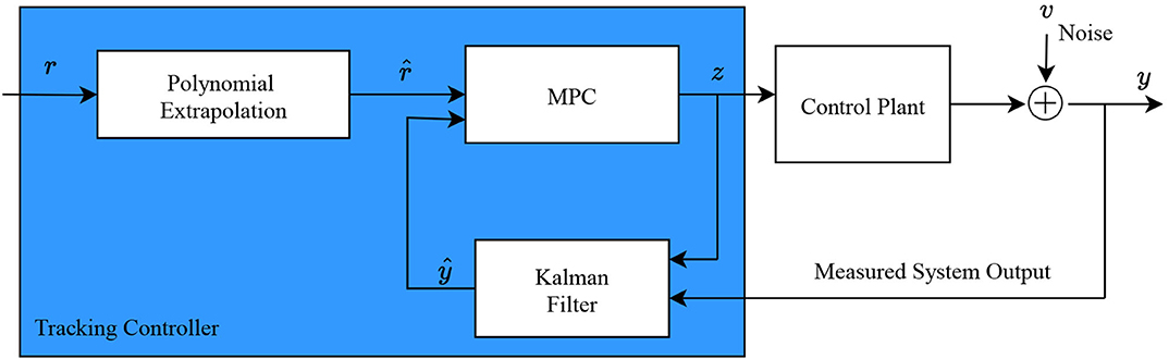
Figure 1. Architecture of the proposed tracking controller.

2.1. Model Predictive Control

Model Predictive Control (MPC) is a control strategy in which the ongoing control law is adapted by computing, at every control interval, a finite horizon optimization problem, applying the ongoing state of the control plant as the initial state. The optimization generates an optimal control sequence consisting of a series of individual control laws, out of which the first one is applied to the control plant for the current control interval (Mayne et al., 2000). The control interval is defined as a sampling instant or, in other words, as a set of continuous time steps of the simulation, serving as an internal time step for the MPC in to order to gather sufficient feedback measurements to accurately predict future control plant outputs and to advance the optimization to the next control sequence. In MPC, a standard finite horizon optimal control problem is being solved similar to H_∞ and LQR control approaches. In H_∞ and LQR control, the optimal problem could be of infinite horizon as well, while that's not the case for MPC. What differs, nonetheless, is the fact that in MPC new control laws are computed in each control interval, whilst in classical control theory a single control law, which is computed offline prior to the simulation, is used for the whole duration of the simulation. This is the fundamental difference between MPC and classical control theory. Online control law derivation is also a feature of adaptive control theory. However, in the latter, conducting system identification needed for the adaptive controller can cause numerical delays, whilst in MPC the model used in the controller remains the same and therefore no identification is needed. Changing online the parameters of the model used in MPC would result in the so-called adaptive MPC, but this is not part of this study.

Every application imposes mandatory (hard) constraints. For example: (i) actuators are of limited stroke/capacity meaning that the produced displacement/force is limited; and/or (ii) safety limits are applied in almost every experimental setup. The problem of meeting hard constraints in control applications is well established in the literature. MPC has proven to be one of the few adequate control methodologies to suitably satisfy constraints on the inputs, states and/or outputs of the system under consideration, maintaining concurrently the desired performance (Zafiriou, 1990).

The proposed tracking MPC controller consists of four elements; (a) the prediction model, (b) the performance index or cost function, (c) the constraints, and (d) a solver to derive the control laws. The prediction model serves as the core of MPC since it is responsible for the future predictions of the control plant outputs, taking into account the past and present values of the computed optimal control laws. The prediction model should be as accurate as possible in order to be able to sufficiently capture the control plant dynamics and its behavior. Therefore, a detailed prediction model could improve MPC performance. However, there is a trade-off between the complexity of the prediction model and the computational power needed to compute it at every control interval. Care must be taken in order not to introduce delays due to numerical calculations, especially in real-time applications, as RTHS, in which timing is crucial.

The MPC methodology used in this study is described below and illustrated in Figure 2B. In Figure 2A, the structure of the MPC controller is shown. At each control interval k, MPC optimizes the control plant outputs y_j. Namely, the future outputs $\widehat{y}$(k + i|k), for k = 0, …, P of a predefined prediction horizon P are predicted at each control interval k using the prediction model. The i-th prediction horizon step is a time instant of the current control interval k. The latter depends on the known values up to this k and on the future control laws u(k + i|k), for k = 0, …, P − 1. The control sequence $z_k^T=[u{(k|k)}^T\dots u{(k+i|k)}^T\dots u{(k+P-1|k)}^T]$ consists of a sequence of control laws u(k + i|k). It is calculated by optimizing a quadratic cost function at each k. The cost function embodies the tracking error, i.e., the error between the reference trajectory and the predicted output values of the control plant, and is expressed as follows:

$\begin{array}{l}{\text{J}}^{*}({\widehat{r}}_k,{\widehat{y}}_k,z_k)={\displaystyle \sum _{j=1}^{n_y}}{\displaystyle \sum _{i=1}^P}{\{w^{y_j}[{\widehat{r}}_j(k+i|k)-{\widehat{y}}_j(k+i|k)]\}}^2+\\ \begin{array}{l}{\displaystyle \sum _{j=1}^{n_u}}{\displaystyle \sum _{i=0}^{P-1}}{\{w^{u_j}[u_j(k+i|k)-u_j(k+i-1|k)]\}}^2\end{array}& (1)\end{array}$

where n_y correspond to the number of control plant outputs, n_u the number of control plant inputs, ${\widehat{r}}_j(k+i|k)$ the reference value to be tracked at the i-th prediction horizon step from the j-th control plant output, $\widehat{y}$_j(k + i|k) the predicted value of the j-th control plant output at the i-th prediction horizon step, u_j(k+i|k) the j-th control plant input at the i-th prediction horizon step, $w^{y_j}$ the tuning weight of the j-th control plant output and $w^{u_j}$ the tuning weight of the j-th control plant input. (i|k) represents the current step i of the prediction horizon P at the control interval k.

FIGURE 2

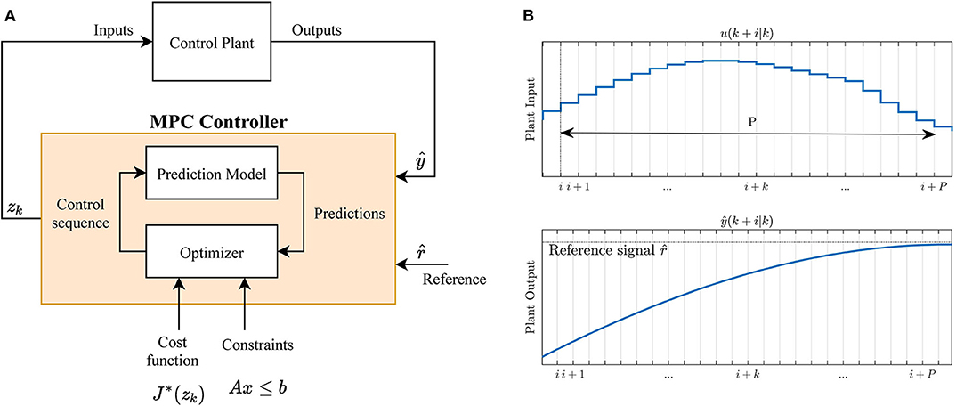
Figure 2. (A) MPC structure of the tracking controller, (B) MPC methodology.

Additionally, in the proposed tracking controller an output disturbance model w is used as described in Equation (2). The input of the model u_w, is assumed to be white noise and the disturbance w is additive to the control plant outputs. The disturbance model is used to include potential unmeasured noise that could occur during RTHS, e.g., experimental measurement errors. In the proposed design, the disturbance model follows:

$\begin{array}{l}{x}_w(k+1)=A_w{x}_w(k)+B_w{u}_w(k)\\ \begin{array}{l}w(k)=C_w{x}_w(k)+D_w{u}_w(k)\end{array}& (2)\end{array}$

where A_w, B_w, C_w, and D_w are matrices associated with the disturbance w.

The $k,P,w^{y_j},\text{and }{w}^{u_j}$ parameters from Equation (1) remain constant for the entire RTHS. MPC constantly receives reference trajectories, ${\widehat{r}}_j(k+i|k)$, for the whole prediction horizon P, which in RTHS corresponds to the outputs of the numerical substructure and uses the prediction model along with the Kalman filter (see section 2.2) to predict the control plant outputs, $\widehat{y}$_j(k+i|k), which depend on the control sequence z_k, the disturbance w(k) and the Kalman filter's estimates. The control sequence z_k is computed in the optimizer (see Figure 2A), which takes into account the cost function (and in essence the tracking error, as it's embedded in the cost) and the constraints. The quadratic cost function of Equation (1) can be transformed into a Quadratic Programming (QP) problem (Delbos and Gilbert, 2003; Tøndel et al., 2003) and this is what is essentially being solved in the optimizer. The QP problem is formulated as follows:

$\begin{array}{ll}{\displaystyle \underset{x}{\text{min}}}(\frac{1}{2}{x}^{T}Hx+f^{T}x)& (3)\end{array}$

$\begin{array}{ll}\text{subject to }Ax\le b& (4)\end{array}$

where the Ax ≤ b inequality corresponds to the constraints applied, x is the solution vector, H the Hessian matrix, A is a matrix of linear constraints coefficients, b is a vector relevant with the constraints, and f is a vector obtained by:

$\begin{array}{ll}f=K{x}^T{x}_{kf}(k|k)+Kr{(k|k)}^{T}r(k|k)+Ku{(k|k-1)}^{T}u(k|k-1)& (5)\end{array}$

where $x_{kf}^T=\left[\begin{array}{cc}{x}_p^T& x_w^T\end{array}\right]$ is the vector corresponding to the states of the Kalman filter (see section 2.2) and consists of the control plant states x_p and of the disturbance w states x_w, r(k|k) is the reference signal at the current control interval, u(k|k − 1) is the control law applied to the control plant in the previous control interval and K a weighting factor.

In the proposed tracking controller, an active-set solver applying the KWIK algorithm (Schmid and Biegler, 1994) is used for solving the QP problem. This is a built-in QP solver from the Model Predictive Toolbox of MATLAB, used in this study to derive the control law sequence.

The MPC algorithm used in the proposed tracking controller can be summarized as follows:

1. Assuming the output disturbance model from Equation (2), consider a discrete-time multiple-input-multiple-output (MIMO), linear time invariant (LTI) system, representing a linearized model of the control plant:

$\begin{array}{l}{x}_p(k+1)=A_p{x}_p(k)+B_{p}u(k)\\ \begin{array}{l}y(k)=C_p{x}_p(k)+D_{p}u(k)+D_{pw}w(k)\end{array}& (6)\end{array}$

where A_p, B_p, C_p, D_p, and D_pw are matrices corresponding to the control plant. This is the prediction model used along with estimates from the Kalman filter (see section 2.2) to provide MPC with predictions of future control plant outputs.

2. MPC performs the optimization at every control interval k = 0, 1, …:

$\begin{array}{ll}{\displaystyle \underset{z_k}{\text{min }}}{\text{J}}^{*}({\widehat{r}}_k,{\widehat{y}}_k,z_k)& (7)\end{array}$

$\begin{array}{ll}\text{subject to }{u}_{j_{min}}\le u_j\le u_{j_{max}}\text{ and}& (8)\end{array}$

$\begin{array}{ll}{\stackrel{.}{u}}_{j_{min}}\le {\stackrel{.}{u}}_j\le {\stackrel{.}{u}}_{j_{max}}& (9)\end{array}$

where the above constraints correspond to the physical limitations of the actuator regarding displacement and velocity capacity and ${\text{J}}^{*}({\widehat{r}}_k,{\widehat{y}}_k,z_k)$ to the cost of Equation (1). The above limitations/capacities of the actuator are implemented as internal hard constraints of MPC. As a result, MPC guarantees, for the case studies addressed in section 3, that the performance of the controller is not affected by how close the actuator is to its limits.

3. The control sequence $z_k^T=[u{(k|k)}^T\dots u{(k+i|k)}^T\dots u{(k+P-1|k)}^T]$ is obtained for every control interval k:

$\begin{array}{ll}{z}_k:=\text{arg min }{\text{J}}^{*}({\widehat{r}}_k,{\widehat{y}}_k,z_k)& (10)\end{array}$

from the QP solver and it's applied to the control plant.

4. Steps 1–3 are repeated until the end of the RTHS.

In RTHS, the uncertainties and experimental errors are neither constant nor predictable. MPC enables computing a new control law for every control interval within the simulation time, making it possible to compensate specifically for the incurred time delays, uncertainties and/or experimental errors that are introduced in RTHS at each specific control interval. In contrast, classical control techniques utilize a single pre-computed control law that is robust enough to compensate for all the delays coming into play in the entire simulation process. In addition, RTHS always involves experimental equipment, which has physical boundaries, e.g., limited actuator force capacity. Hence, the command signals must be limited to satisfy these boundaries. MPC can solve optimization problems and concurrently satisfy hard constraints, which in the RTHS case, can be laboratory limitations. The aforementioned points make MPC desirable and suitable for RTHS applications. In the case studies presented in the following sections, the selection of the control interval k, the prediction horizon P, and the weights $w^{y_j}$ and $w^{u_j}$ is made through trial and error as there exists a trade-off between optimal controller performance and computational effort. Selection of the above MPC parameters is case study dependent. However, for control interval k and prediction horizon P, the following rules may be applied as a first trial (Bemporad et al., 2020):

• obtain each k at a sampling rate T_s, between 10 and 25% of the minimum desired closed-loop response time. A radical decrease of T_s will result in computational effort increase. T_s cannot be smaller than the sampling rate of RTHS.

• set P such that the desired closed-loop response time T, is approximately equal to PT_s, and the controller is internally stable.

• further optimization of the controller should be done through tuning of the weight coefficients w, but not through tuning of P.

MPC theory is quite extensive, covering various subjects (e.g., convex optimization, optimal control theory, computational solvers) that are taken into account during the design and implementation process of MPC and are not described in full detail in this paper. For a more comprehensive literature in MPC, the reader is encouraged to consult (Bitsoris, 1988; Rossiter, 2003; Boyd and Vandenberghe, 2004; Camacho and Bordons, 2007; Rawlings et al., 2017).

2.2. Kalman Filter

As mentioned above, good accuracy of the predicted control plant outputs is significant as it affects the performance of MPC. In order to improve the predictions' accuracy, a Kalman filter is implemented to estimate the future control plant output values. The purpose of the Kalman filter is to estimate how the current control law will alter the future control plant outputs and use these estimations to optimize the control sequence. The Kalman filter state-space formulation used in MPC follows:

$\begin{array}{l}{x}_{kf}(k+1)=A_{kf}{x}_{kf}(k)+B_{kf}{u}_{kf}(k)\\ \begin{array}{l}\widehat{y}(k)=C_{kf}{x}_{kf}(k)+D_{kf}{u}_{kf}(k)\end{array}& (11)\end{array}$

where

$\begin{array}{l}{A}_{kf}=\left[\begin{array}{cc}{A}_p& 0\\ 0& A_w\end{array}\right],B_{kf}=\left[\begin{array}{cc}{B}_p& 0\\ 0& B_w\end{array}\right]\\ \begin{array}{l}{C}_{kf}=\left[\begin{array}{cc}{C}_p& C_w\end{array}\right],D_{kf}=\left[\begin{array}{cc}0& D_w\end{array}\right]\text{ and}\\ u_{kf}^T=\left[\begin{array}{cc}{z}_k^T& u_w{(k)}^T\end{array}\right]\end{array}& (12)\end{array}$

The weighting coefficients for the Kalman filter are derived from the following expectations:

$\begin{array}{l}Q=𝔼[B_{kf}{u}_{kf}{u}_{kf}^T{B}_{kf}^T],R=𝔼[D_{kf}{u}_{kf}{u}_{kf}^T{D}_{kf}^T],\\ \begin{array}{l}N=𝔼[B_{kf}{u}_{kf}{u}_{kf}^T{D}_{kf}^T]\end{array}& (13)\end{array}$

In Figure 1 is illustrated how the Kalman filter is integrated within the proposed tracking controller. More specifically, in the beginning of each control interval k, the state of the Kalman filter, $x_{kf}^T=\left[\begin{array}{cc}{x}_p^T& x_w^T\end{array}\right]$, is estimated for the next interval as follows:

• x_kf(k|k) is updated based on the latest measurements:

$\begin{array}{ll}{x}_{kf}(k|k)=x_{kf}(k|k-1)+M[y(k)-C_{kf}{x}_{kf}(k|k-1)]& (14)\end{array}$

• The state for the next, k + 1, control interval is estimated as:

$\begin{array}{l}{x}_{kf}(k+1|k)=A_{kf}{x}_{kf}(k|k-1)+B_{p}u(k)\\ \begin{array}{l}+L[y(k)-C_{kf}{x}_{kf}(k|k-1)]\end{array}& (15)\end{array}$

where L, M are the Kalman filter gain matrices and u(k) the optimal control law assumed to be used from the control interval (k − 1) until k. y(k) is the measured control plant output at the control interval k.

Once the state for the k + 1 interval is estimated, the values of the control plant output at this interval can be predicted as follows:

• For any successive step, i = 1:P, within the ongoing control interval k, the next state is estimated as:

$\begin{array}{ll}{x}_{kf}(k+i|k)=A_{kf}{x}_{kf}(k+i-1|k)+B_{p}u(k+i-1|k)& (16)\end{array}$

• Hence, the predicted control plant output value is calculated as:

$\begin{array}{ll}\widehat{y}(k+i|k)=C_{kf}{x}_{kf}(k+i|k)\text{, for }i=1,\dots ,P& (17)\end{array}$

where i corresponds to the prediction horizon step.

2.3. Polynomial Extrapolation

MPC can guarantee adequate tracking performance and robustness under uncertainties and disturbances. However, since in RTHS even small tracking errors can significantly alter the simulation outcome, a fourth-order polynomial extrapolation (Horiuchi, 1996; Wallace M. et al., 2005; Wallace M. I. et al., 2005; Ning et al., 2019) is integrated in the tracking controller as illustrated in Figure 1, in order to further compensate for time delays and additionally improve the MPC performance. It's formulation follows:

$\begin{array}{ll}{\widehat{r}}_k=a_0{r}_{(0,k)}-a_1{r}_{(1,k)}+a_2{r}_{(2,k)}-a_3{r}_{(3,k)}+a_4{r}_{(4,k)}& (18)\end{array}$

where r_{(i, k)} = r(t_k − iT_d) is the discrete reference signal by adding shifts of a pure time delay T_d by integer values of i. The polynomial coefficients a₀ - a₄ are obtained using the Lagrange basis function by trial and error.

3. Case Studies

The following two virtual RTHS parametric case studies (CS) serve as validation for the performance and robustness of the proposed tracking controller. The case studies are virtual in that both the physical substructures of the hybrid models are implemented numerically in software, not physically as specimens in a laboratory. This was done to facilitate the development and testing of the proposed MPC. For each case study, the dynamics of the tested system are explained, then the tracking controller design properties are addressed and finally, results are presented. Since the goal of each case study is to examine the behavior of the tracking controller, the outputs of the hybrid models are exclusively related to the controller's performance. The outputs will be:

1. Tracking time-delay, defined as:

$\begin{array}{ll}{J}_1=\left(\underset{k}{\text{arg max}}\right(\text{Corr}(r(i),y(i-k))\left)\right)f_{RTHS}[\text{msec}]& (19)\end{array}$

where f_RTHS is the sampling frequency of RTHS.

2. Normalized Root Mean Square (NRMS) of the tracking error, defined as:

$\begin{array}{ll}{J}_2=\sqrt{\frac{{\displaystyle {\sum }_{i=1}^N}[y(i)-r(i){]}^2}{{\displaystyle {\sum }_{i=1}^N}[r(i){]}^2}}\times 100\text{ [\%]}& (20)\end{array}$

3. Peak Tracking Error (PTE), defined as:

$\begin{array}{ll}{J}_3=\frac{\text{max}|y(i)-r(i)|}{\text{max}|r(i)|}\times 100\text{ [\%]}& (21)\end{array}$

J₁ is established as the maximum cross-correlation between the reference and the measured signal, multiplied by the sampling frequency of RTHS. It is a metric of how different in time these two signals are. The cross-correlation describes how many time steps the measured signal should be shifted in order to match the reference. When J₁ > 0 the measured signal is delayed with respect to the reference (tracking delay), whilst when J₁ < 0, the measured signal is leading the reference (overcompensation). The desire is to have zero time tracking delay, meaning the value of J₁ to be as close to zero as possible, without overcompensating. J₂ represents how quantitatively different the reference and measured signals are accounting for the whole simulation period, whilst J₃ accounts only for the maximum value of the tracking error. The performance of the tracking controller is assessed by how close to zero J₁, J₂, and J₃ are (Silva et al., 2020).

3.1. CS1: vRTHS of a Structure With an Attached Pendulum

3.1.1. Problem Formulation

The reference system under consideration for CS1 corresponds to a vertical cantilever beam with mass concentrated at its top, and a pendulum attached to the center of gravity of the cantilever mass, as shown in Figure 3A. The numerical substructure is the cantilever beam (Figure 3B), described by Equation (22), while the virtual physical substructure is the pendulum (Figure 3C).

FIGURE 3

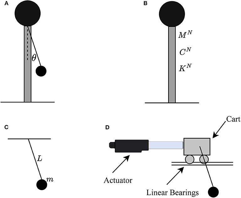
Figure 3. Hybrid model of CS1: (A) Reference structure, (B) Numerical substructure, (C) Virtual physical substructure, (D) Control plant.

The Equation of Motion (EoM) for the reference structure follows:

$\begin{array}{ll}{M}^N\ddot{x}+C^N\stackrel{.}{x}+K^{N}x=-M^N{\ddot{x}}_g+f^P& (22)\end{array}$

where $\ddot{x}$, $\stackrel{.}{x}$, and x correspond to acceleration, velocity and displacement of the numerical substructure relative to the ground, M^N = 100 [Kg], $C^N=100\left[\frac{Ns}{m}\right]$, and $K^N=10e4\left[\frac{N}{m}\right]$ are mass, damping and stiffness of the numerical substructure respectively, $\ddot{x}$_g is the ground motion applied to the hybrid model and f^P the force measured from the virtual physical substructure.

The virtual physical substructure corresponds only to the pendulum. However, to move the pendulum pivot point horizontally in a lab, an actuator could be attached to a cart mounted on a horizontal rail. Thus, the cart and the actuator would be the transfer system. As a result, the cart dynamics and its interaction with the pendulum are taking into account for solving the equations for the virtual physical substructure. The virtual physical substructure is described by the Equations (23) and (24). Moreover, in order to reduce as much as possible the friction due to the cart movement μ, low friction linear bearings are assumed to be implemented. The friction at the pendulum pivot, b, is assumed to be small.

The EoM for the cart with the pendulum follows:

$\begin{array}{ll}\ddot{x}=\frac{m{L}^2{\stackrel{.}{\theta }}^2\text{sin}(\theta )+mLg\text{ sin}(\theta )\text{ cos}(\theta )+\stackrel{.}{\theta }b\text{ cos}(\theta )-\mu L\stackrel{.}{x}+f^{P}L}{L(m{\text{ sin}}^2(\theta )+M)}& (23)\end{array}$

$\begin{array}{ll}\ddot{\theta }=\frac{\begin{array}{l}-m{L}^2{\dot{\theta }}^2\text{ sin}(\theta )\text{ cos}(\theta )-\dot{\theta }b(1+\frac{M}{m})\hfill \\ -gL(M+m)\text{ sin}(\theta )+\dot{x}L\mu \text{ cos}(\theta )+f^{P}L\text{ cos}(\theta )\hfill \end{array}}{L^2(m{\text{sin}}^2(\theta )+M)}& (24)\end{array}$

where the parameters from Equations (23) and (24) correspond to:

• Pendulum angle, angular velocity, angular acceleration $\to \theta ,\stackrel{.}{\theta },\ddot{\theta }$, respectively

• Cart position, velocity, acceleration → x, $\stackrel{.}{x}$, $\ddot{x}$, respectively

• Force generated from the pendulum → f^P

• Pendulum mass → m = 0.15[Kg]

• Cart mass → M = 2[Kg]

• Rod length → L = 0.7[m]

• Cart friction coefficient → μ = 0.001[-]

• Pendulum friction coefficient → b = 0.0001[-]

• Acceleration of gravity $\to g=9.81\left[\frac{m}{s^2}\right]$.

Since this is a virtual simulation, an actuator model needs to be implemented representing the dynamics of the real actuator. For CS1, a linear hydraulic actuator was chosen. Its model consists of three transfer functions; (i) G_sv represents the servo-valve dynamics as in Equation (25), (ii) G_a the actual actuator dynamics as in Equation (26), and (iii) G_CSI the control-structure-interaction (CSI) (Dyke et al., 1995) as in Equation (27). The way these transfer functions are interconnected is shown using a block diagram of the actuator model in Figure 4. Taking the above into consideration, the control plant for CS1, corresponds to the actuator model along with the cart and the pendulum. A graphical representation of the control plant is illustrated in Figure 3D and it's block diagram in Figure 4. The control plant is a single-input-multiple-output (SIMO) model with input the displacement of the actuator z and four outputs; $x,\stackrel{.}{x},\theta ,\text{ and }\stackrel{.}{\theta }$. In the tracking controller, only the first output, the cart position x is used, described by a single-input-single-output (SISO) transfer system as in Equation (28).

$\begin{array}{ll}{G}_{sv}=\frac{2.128e13}{s^2+425s+99976}& (25)\end{array}$

$\begin{array}{ll}{G}_a=\frac{1}{s+3.3}& (26)\end{array}$

$\begin{array}{ll}{G}_{CSI}=7.26e5s& (27)\end{array}$

$\begin{array}{ll}{G}_{cp}=\frac{0.5s^2+0.0007823s+8.058}{s^4+0.001963s^3+15.07s^2+0.007s}& (28)\end{array}$

The block diagram of the overall hybrid model is presented in Figure 5A. It consists of the numerical and virtual physical substructures, the proposed tracking controller and the control plant. The RTHS is conducted in displacement control; in every time step the measured displacement of the cart (same as the horizontal displacement of the pendulum), x, is fed back in the tracking controller, while the measured force generated from the movement of the pendulum, f^P is fed back to the numerical substructure to compute the next displacement command r. The coupling of the two substructures is achieved through force f^P. Furthermore, apart from the disturbance described in Equation (2), in order to capture even more realistic results, additional white noise v is added in the calculated displacement x and force f^P, representing measurement noise from the displacement and force sensors, respectively. The displacement and force sensor noise is modeled with two correlated standard Gaussian distributions, generated at the same frequency as the sampling of RTHS and amplified each by 1.5e-7 m and 6e-5 N, respectively, which approximately equals to 0.01% of the respective full spans. The sampling frequency of RTHS was set to f_RTHS = 4, 096Hz. For the numerical integration scheme, the RK4 (fourth-order Runge–Kutta) method is used with a fixed time step of 1/4, 096 s. The reference ground motion of the hybrid model $\ddot{x}$_g is a historical acceleration record from the El Centro 1940 earthquake downscaled by 0.4, as shown in Figure 6A. In Figure 6B, the power spectral density of the respective record is illustrated.

FIGURE 4

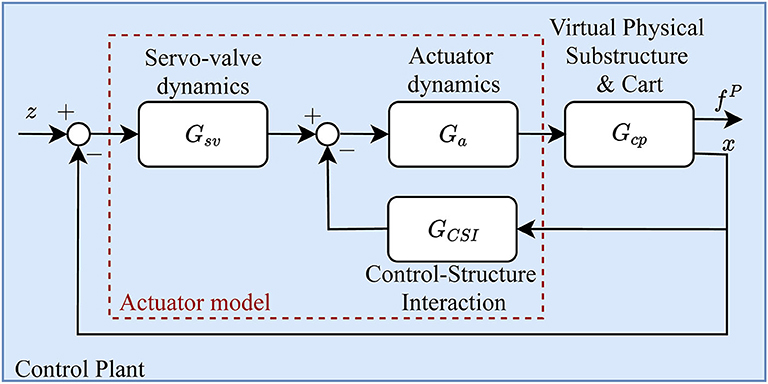
Figure 4. Block diagram of the control plant in CS1.

FIGURE 5

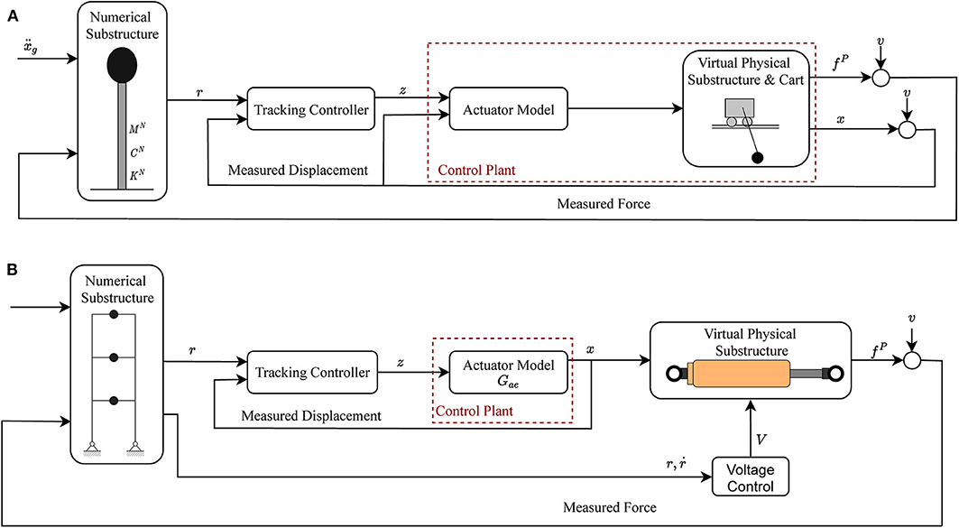
Figure 5. Block diagrams of hybrid models: (A) CS1, (B) CS2.

FIGURE 6

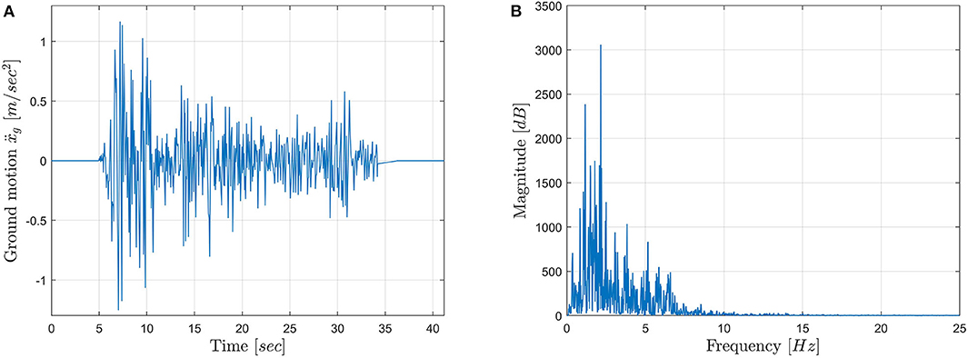
Figure 6. Reference ground motion used in CS1 & CS2; El Centro 1940 earthquake North-South ground motion record, downscaled by 0.4: (A) Time-series and (B) Power spectral density of the respective record.

3.1.2. Tracking Controller Design Properties

The prediction model used in MPC for CS1 is a linearized model of the control plant. Since MPC functions in discrete time, the linearized model of the control plant is discretized with the sampling frequency of RTHS, f_RTHS. Essentially it's a discrete LTI SISO model described using the state-space formulation as follows:

$\begin{array}{l}x(k+1)=A_{p}x(k)+B_{p}u(k)\\ \begin{array}{l}y(k)=C_{p}x(k)+D_{p}u(k)+D_{pw}w(k)\end{array}& (29)\end{array}$

where A_p, B_p, C_p, D_p, and D_pw = 1 are the prediction model matrices, equal to:

$\begin{array}{l}{A}_p=\left[\begin{array}{ccccccc}0.4762& -0.3993& -0.2475& -0.2307& -0.2279& -0.0009& -0.0143\\ 0.7532& 0.7912& -0.1315& -0.1222& -0.1272& -0.0005& -0.008\\ 0.2103& 0.4645& 0.9775& -0.0209& -0.0223& 0& -0.0014\\ 0.0184& 0.0603& 0.2486& 0.9987& -0.0014& 0& 0\\ 0.0012& 0.0051& 0.0312& 0.2499& 1& 0& 0\\ 0& 0& 0.0002& 0.002& 0.0156& 1& 0\\ 0& 0& 0& 0& 0.0001& 0.0156& 1\end{array}\right],\\ \begin{array}{l}{B}_p=\left[\begin{array}{c}0.0118\\ 0.0066\\ 0.0012\\ 0\\ 0\\ 0\\ 0\end{array}\right]\end{array}\\ \begin{array}{l}{C}_p=\left[\begin{array}{ccccccc}0& 0& 0& 0& 19.86& 0.002& 1.25\end{array}\right],D_p=\left[0\right]\end{array}& (30)\end{array}$

The disturbance model used, expressed by Equation (2), is added to the control plant output and its model follows:

$\begin{array}{l}{x}_w(k+1)=x_w(k)+0.0009766u_w(k)\\ \begin{array}{l}w(k)=x_w(k)\end{array}& (31)\end{array}$

with A_w = 1, B_w = 0.0009766, C_w = 1, and D_w = 0.

The Kalman filter gain matrices follow:

$\begin{array}{l}L={\left[\begin{array}{cccccccc}0.0096& -0.0062& -0.0269& 0.0021& 0.0148& 0.0004& -0.0003& 0.0008\end{array}\right]}^T\\ \begin{array}{l}M={\left[\begin{array}{cccccccc}0.0071& -0.0147& -0.0215& 0.0082& 0.0135& 0.0002& -0.0003& 0.0008\end{array}\right]}^T\end{array}& (32)\end{array}$

Starting with Equations (30), (31), and (32) the derivation of the Kalman filter formulation in Equation (11) is straightforward. The MPC weight coefficients used in Equation (1) are selected to be w^y = 15.26 and w^u = 0.63. The number of control plant outputs n_y is 1 and the number of control plant inputs n_u, is also 1. The prediction horizon was set to P = 8 and each control interval k was obtained at a sampling frequency of 1, 024Hz, one fourth of the RTHS sampling rate. The constraints applied represent the physical limitations of the actuator to provide bounded displacements and velocity. It's assumed that the virtual actuator has a maximum stroke of ±250 [mm] and maximum velocity of ±100 $\left[\frac{mm}{sec}\right]$. So the constraints follow:

$\begin{array}{l}-250\le \widehat{z}(k+i|k)\le 250,[mm]\text{ for }i=1,\dots ,P\\ \begin{array}{ll}-100\le & \stackrel{.}{\widehat{z}}(k+i|k)\le 100,[\frac{mm}{sec}]\text{ for }i=1,\dots ,P\end{array}& (33)\end{array}$

The polynomial extrapolation coefficients used in CS1 for the proposed tracking controller follow:

$\begin{array}{ll}{\widehat{r}}_k=5r_{(0,k)}-10r_{(1,k)}+10r_{(2,k)}-5r_{(3,k)}+r_{(4,k)}& (34)\end{array}$

3.1.3. CS1 Results

In order to test the robustness of the proposed tracking controller, six dominant parameters of the hybrid model were chosen to vary. The first three parameters originate from the control plant and correspond to its M, m, and L, while the remaining three originate from the numerical substructure and correspond to its M^N, C^N, and K^N. These parameters are treated as random with known probability distributions. Their distribution characteristics are described in Table 1.

TABLE 1

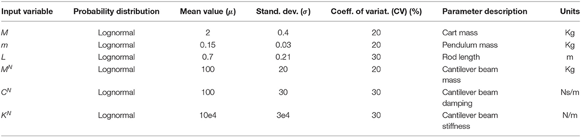
Table 1. CS1: Variation of the random parameters in the hybrid model.

Using the Latin Hypercube Sampling (LHS) methodology, 200 samples were generated from all six parameters and 200 runs of the vRTHS were conducted using combinations of all parameters in each iteration. The tracking controller was kept the same for each one of the 200 runs. The simulation of the 200 vRTHS runs is referred as stochastic vRTHS hereafter. The resulting J₁, J₂, and J₃ outputs of the nominal and the stochastic vRTHS are shown in Table 2 for both CS1 and CS2 for brevity. The nominal values correspond to the parameters used in Equations (22), (23), and (24). The normalized histograms of the J₁, J₂, and J₃ out of the 200 vRTHS are shown in Figure 7. The aforementioned histograms are a more comprehensive, graphical representation of the values presented in Table 2, illustrating the mean values as well as the deviations from them. It is also a metric of robustness; more robust tracking controllers would result in lower deviations in the histograms.

TABLE 2

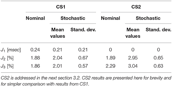
Table 2. Tracking controller performance and robustness results for CS1 and CS2.

FIGURE 7

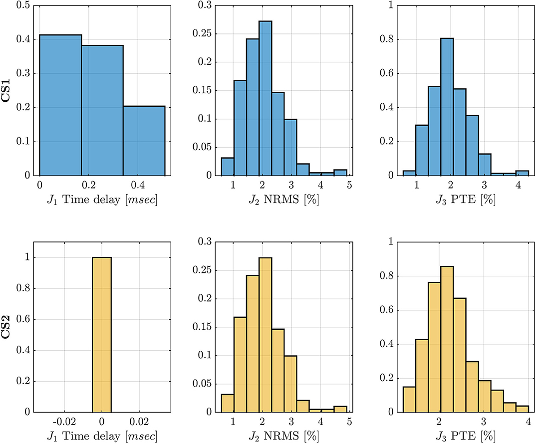
Figure 7. Normalized histograms of J₁, J₂, and J₃ for CS1 and CS2, obtained from 200 vRTHS runs.

Analysis of the results using uncertainty quantification techniques indicated that 200 runs were sufficient to unveil how the tracking controller performance is affected by parameter variations. Specifically, surrogate models were developed to replicate the response of the CS as the number of runs (in the surrogate training data set) was increasing. With a training data set of 200 samples, validation errors of the surrogate models were <5%. No new runs were added to the data set as this error was deemed to be sufficiently small.

To check if the proposed tracking controller remains stable as the hybrid model parameters vary, vRTHS simulations using the minimum and the maximum values of the random variables were conducted first. No instabilities were observed. Furthermore, none of the conducted 200 simulations was unstable. The same holds for CS2.

The reference, command and measured signals of the hybrid model in the nominal vRTHS are illustrated in Figure 8. The reference signal corresponds to the displacement response of the reference model (one with integrated physical and numerical substructures). The command signal corresponds to the displacement response r computed from the numerical substructure at each given time step of vRTHS and is the one that should be followed from the control plant. Finally, the measured signal corresponds to the measured displacement response x of the virtual physical substructure. An ideal tracking controller should be able to compensate the hybrid model in such a way that the command r and measured x to be identical. As it's shown from Figure 8, those two signals are, indeed, very close. The comparison with the reference signal is provided in order to validate the fidelity of the hybrid model with respect to the reference structure.

FIGURE 8

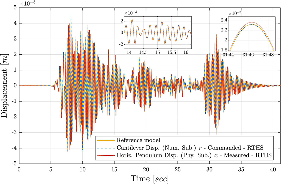
Figure 8. Displacement responses of the reference model and of the numerical and physical vRTHS substructures in CS1.

In Figure 9, the performance index of the MPC versus time for the nominal case is displayed. This graph illustrates how well MPC managed to minimize the given objective cost function of Equation (1) in every time step of the simulation. A zero value would mean that the cost function was minimized as desired and the “best” optimal control sequence was computed for the given time step. From Figure 9, we can observe that the performance index is almost zero during the entire vRTHS, while it is not zero in the time steps in which the highest peaks of the reference signal are attained. This is expected, as the peaks of the command signal are approached, the controller is challenged more and more and has to adapt.

FIGURE 9

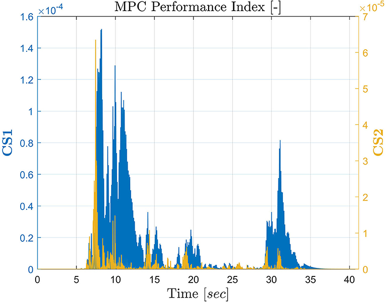
Figure 9. MPC optimization performance index for CS1 and CS2.

Since the performance of the tracking controller is assessed by how close to zero J₁, J₂, and J₃ are, it's clear from Table 2 and Figures 7–9 that the proposed tracking controller can provide the desired performance under the presence of any combination of all six random parameters of the hybrid model chosen here, which also demonstrates its robustness. The effects of these stochastic parameters could represent the effect of potential uncertainties (aleatory and/or epistemic) that could be introduced during RTHS. On top of that, it should be pointed out that the controller maintains its performance even in the presence of the additional noise v and disturbance w that were added in the hybrid model.

3.2. CS2: vRTHS of a Magnetorheological Damper Attached to a 3-Story Structure

3.2.1. Problem Formulation

The reference structure in CS2 corresponds to a 3-story structure equipped with a magnetorheological damper (MRD), installed between the ground and first floor (Dyke et al., 1998) as shown in Figure 10A. The numerical substructure corresponds to the 3-story structure (Figure 10B), while the virtual physical to the MRD (Figure 10C).

FIGURE 10

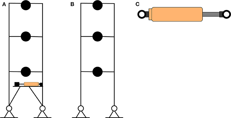
Figure 10. Hybrid model of CS2: (A) Reference structure, (B) Numerical substructure, (C) Virtual physical substructure.

The EoM of the reference model reads:

$\begin{array}{ll}{\text{M}}^N\ddot{\text{x}}+{\text{C}}^N\stackrel{.}{\text{x}}+{\text{K}}^N\text{x}=-\text{M}\Lambda {\ddot{x}}_g+\Gamma f^P& (35)\end{array}$

where $\text{x}={[x_1,x_2,x_3]}^T$, $\stackrel{.}{\text{x}}={[{\stackrel{.}{x}}_1,{\stackrel{.}{x}}_2,{\stackrel{.}{x}}_3]}^T$, and $\ddot{\text{x}}={[{\ddot{x}}_1,{\ddot{x}}_2,{\ddot{x}}_3]}^T$ correspond to the displacement, velocity, and acceleration relative to the ground, $\ddot{x}$_g is the ground motion and f^P corresponds to the force generated from the MRD. The M^N, C^N, K^N matrices represent the mass, damping and stiffness of the 3-story structure, respectively, as follows:

$\begin{array}{l}{\text{M}}^N=\left[\begin{array}{ccc}1,000& 0& 0\\ 0& 1,000& 0\\ 0& 0& 1,000\end{array}\right][Kg],\\ {\text{C}}^N=1e4*\left[\begin{array}{ccc}1.408& -0.787& 0.044\\ -0.787& 1.494& -0.635\\ 0.044& -0.635& 0.722\end{array}\right]\\ {\text{K}}^N=1e7*\left[\begin{array}{ccc}2.605& -2.313& 0.594\\ -2.313& 3.256& -1.442\\ 0.594& -1.442& 0.927\end{array}\right][\frac{N}{m}]& (36)\end{array}$

Vector Λ = ${\left[\begin{array}{ccc}1& 1& 1\end{array}\right]}^T$ is the ground motion influence vector, while vector Γ = ${\left[\begin{array}{ccc}1& 0& 0\end{array}\right]}^T$ represents the effect of the MRD on the structure. In RTHS, a state-space representation of the Equation (35) is used, which follows:

$\begin{array}{l}\stackrel{.}{x}=Ax+Bu\\ \begin{array}{l}y=Cx+Du\end{array}& (37)\end{array}$

where $x={\left[x_1,x_2,x_3,{\stackrel{.}{x}}_1,{\stackrel{.}{x}}_2,{\stackrel{.}{x}}_3\right]}^T$, $u={\left[{\ddot{x}}_g,f^P\right]}^T$, $y={\left[x_1,x_2,x_3,{\stackrel{.}{x}}_1,{\stackrel{.}{x}}_2,{\stackrel{.}{x}}_3,{\ddot{x}}_1,{\ddot{x}}_2,{\ddot{x}}_3\right]}^T$, and

$\begin{array}{l}A=\left[\begin{array}{cc}0& I\\ -M^{N^{-1}}{K}^N& -M^{N^{-1}}{C}^N\end{array}\right],B=\left[\begin{array}{cc}0& 0\\ -\Lambda & -M^{N^{-1}}\Gamma \end{array}\right]\\ \begin{array}{l}C=\left[\begin{array}{cc}I& 0\\ 0& I\\ -M^{N^{-1}}{K}^N& -M^{N^{-1}}{C}^N\end{array}\right],D=\left[\begin{array}{cc}0& 0\\ 0& 0\\ -\Lambda & -M^{N^{-1}}\Gamma \end{array}\right]\end{array}& (38)\end{array}$

The block diagram of the hybrid model of CS2 is shown in Figure 5B. The reference signal r, in Figure 5B, corresponds to the displacement of the first story x₁. Respectively, ṙ = $\stackrel{.}{x}$₁. RTHS is conducted in displacement control, as in CS1. The ground motion applied to the hybrid model is the same as in CS1, a historical acceleration record from the El Centro 1940 earthquake downscaled by 0.4. As in CS1, apart from the additive disturbance described in Equation (2), additional white noise v is added in the calculated force from MRD f^P, which represents measurement noise from the load cell. The load cell measurement noise is modeled with a standard Gaussian distribution, generated at the same frequency as the sampling of RTHS and amplified by 0.15 N, which approximately equals to 0.01% of the load cell full span. The sampling frequency of RTHS was set to f_RTHS = 4, 096 Hz. For the numerical integration scheme, the RK4 method is used with a fixed time step of 1/4, 096 s.

To model the virtual physical substructure, the MRD in CS2, the Viscous + Dahl model (Ikhouane and Dyke, 2007) was employed. It's dynamics are described as follows:

$\begin{array}{l}{f}^P(t)=[k_{x_a}+k_{x_b}V(t)]\stackrel{.}{x}(t)+[k_{w_a}+k_{w_b}V(t)]W(t)\\ \begin{array}{l}\stackrel{.}{W}(t)=\rho (\stackrel{.}{x}(t)-|\stackrel{.}{x}|W(t))\\ W(0)=\frac{f^P(0)-[k_{x_a}+k_{x_b}V(0)]\stackrel{.}{x}(0)}{k_{w_a}+k_{w_b}V(0)}\end{array}& (39)\end{array}$

where $\stackrel{.}{x}$(t) denotes the MRD piston velocity, V(t) the voltage input command, f^P(t) the damping force, W the damper's nonlinear behavior, k_xa and k_xb the viscous friction coefficient, k_wa and k_wb the dry friction coefficient and t refers to the simulation time. The parameter ρ is calculated as in Tsouroukdissian et al. (2008) and selected to be ρ = 4, 795(m⁻¹). The friction parameters are calculated from linear regression as $k_{x_a}=978(Ns{m}^{-1}),k_{x_b}=4,075(Ns{m}^{-1}{V}^{-1}),k_{w_a}=160.11(N)$, and $k_{w_b}=500.78(N{V}^{-1})$. The inputs of the MRD model are the displacement x(t) and the voltage V(t), while the output is the force f^P. The latter is the variable that couples the two substructures.

In a MRD, a relatively small electric current applied to the MR valve can change the behavior from very high to very low resistance to motion over a very short time period. In order to ensure optimal response, a bang-bang voltage controller is designed and implemented as illustrated in Figure 5B. More specific, when sgn(r(t)) = sgn(ṙ(t)) then the controller provides the MRD with the maximum input voltage, resulting in maximum MRD force f^P. Otherwise, the MRD force is minimum. This bang-bang controller is part of the MRD and it's exclusively responsible for the internal behavior of the MRD.

In CS2, a different approach of the control plant is investigated compared to CS1, since in this case the control plant corresponds only to the actuator model. In contrast with the control plant represented the actuator model in series with the virtual physical substructure in CS1. Results presented later on prove that the compensation of time delays is sufficient and the performance of RTHS is as desired, when this approach is followed. Moreover, in this way, the dynamics of the control plant are much simpler. Hence, the complexity of the tracking controller is reduced significantly as well. This can be observed by comparing the prediction models used in the two case studies (Equations 30, 40). Therefore, in CS2 the control plant is a SISO model described by Equation (40) with input the desired displacement of the actuator z and output x, the achieved displacement of the actuator. So, in the J₁, J₂, and J₃ criteria the measured signal y(i) of Equations (19), (20), and (21) corresponds to the actuator achieved displacement x. Furthermore, in order to try the proposed tracking controller under different actuator scenarios, the actuator model used in CS2 corresponds to an electric actuator, represented by a second-order transfer function, G_ae, described by the dynamics of Equation (40).

$\begin{array}{ll}{G}_{ae}=\frac{3060}{s^2+267s+3060}& (40)\end{array}$

3.2.2. Tracking Controller Design Properties

As in CS1, the prediction model used in MPC is the control plant, discretized by the sampling frequency of RTHS. The state-space formulation of the discretized model follows (Equation 29) with:

$\begin{array}{ll}{A}_p=\left[\begin{array}{cc}0.7693& -0.0411\\ 0.055& 1\end{array}\right],B_p=\left[\begin{array}{c}0.0069\\ 0.0002\end{array}\right],C_p=\left[\begin{array}{cc}0& 5.98\end{array}\right],D_p=0& (41)\end{array}$

The disturbance model is the same as in Equation (31). The Kalman filter gain matrices in this case are:

$\begin{array}{l}L={\left[\begin{array}{ccc}-0.001& 0.723& 0.974\end{array}\right]}^T*1e(-3)\\ \begin{array}{l}M={\left[\begin{array}{ccc}0.037& 0.721& 0.974\end{array}\right]}^T*1e(-3)\end{array}& (42)\end{array}$

In CS2, the MPC parameters are selected as follows:

• n^y = 1 and n^u = 1

• w^y = 64.073 and w^u = 0.002

• P = 10

• Each control interval k is obtained on a sampling frequency of 1, 024Hz

• The constraints remain the same with Equation (33).

The polynomial extrapolation coefficients are the same as in Equation (34).

3.2.3. CS2 Results

As in CS1, in order to test the robustness of the tracking controller, six dominant parameters are selected to be random variables with known probability distributions. The first four originate from the numerical substructure:

• Beam length → L_b

• Column length → L_c

• Floor mass → M^N

• Damping ratio → Z.

The remaining two parameters correspond to the virtual physical substructure and more specific to K_xa and K_wa. These parameters are of particular importance for the MRD model since they are responsible for its nonlinear behavior. All six parameters along with their distribution characteristics are displayed in Table 3. As in the previous case study, 200 samples are generated with the LHS method from the six parameters, and 200 vRTHS runs are conducted accounting for the variability of all parameters in each run. Again the tracking controller was kept the same in all vRTHSs. The nominal case for CS2 are the parameter values from Equations (37) and (39). The arithmetic results for J₁, J₂, and J₃ can be found in Table 2. Their corresponding normalized histograms for the stochastic vRTHS are illustrated in Figure 7.

TABLE 3

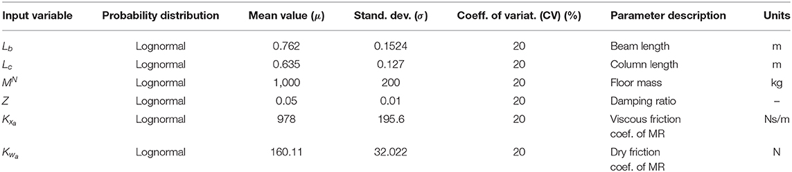
Table 3. CS2: Variation of the random parameters in the hybrid model.

In Figure 11, the force generated by the MRD in the reference model is compared against the one obtained from the vRTHS framework. We can observe that the forces are almost identical. This serves as a demonstration that, although the virtual physical substructure was not included in the control plant, since the latter consists only of the actuator model, its response is compensated sufficiently from time delays and tracking errors. In Figure 12, a comparison between three displacement responses is shown; the displacement response of the reference model, the displacement response of the first floor of the numerical substructure r (this is the command signal to the control plant), and the displacement response x, measured from the control plant [this should track r]. The latter two signals prove that the performance of the tracking controller is as desired, as Figure 12 serves as a graphical illustration of the nominal results shown in Table 2. We can observe that due to the proposed controller, x follows the commanded r with minimum delay and tracking error. Finally, in Figure 9, the performance index of MPC for CS2 is illustrated.

FIGURE 11

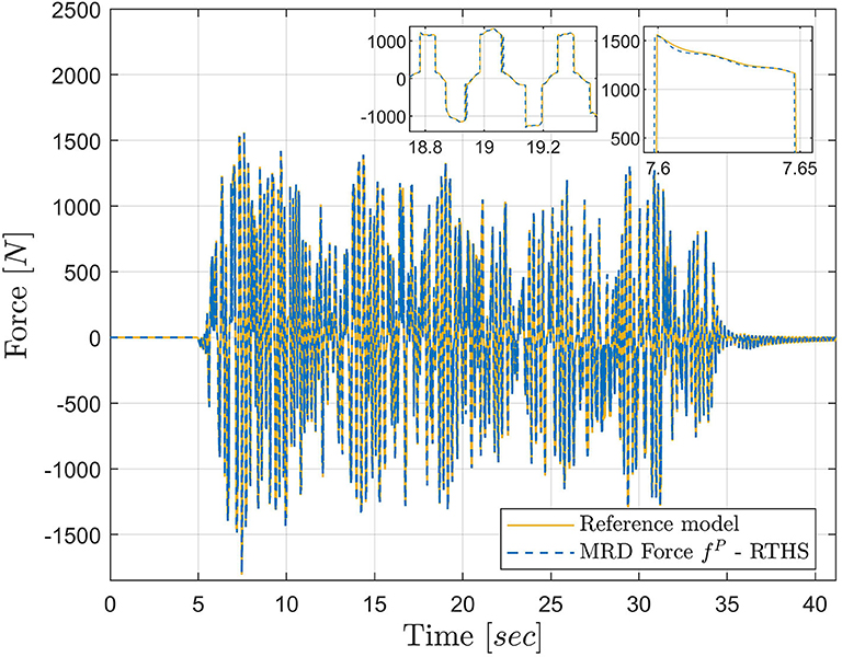
Figure 11. MRD generated force in the reference model and in vRTHS in CS2.

FIGURE 12

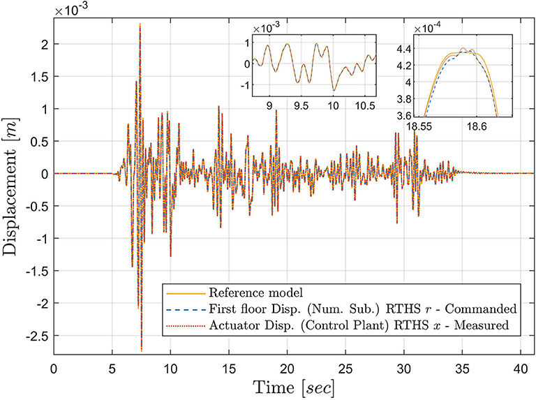
Figure 12. Displacement responses of the reference model, the numerical substructure, and control plant in CS2.

As in the previous case study, from the Table 2, Figures 7, 12, it's shown that the controller performance does not get affected by the presence of the introduced random variables, and it provides the requested performance in all considered cases.

4. Conclusions

In this study, a novel control method to develop a time delay and experimental error compensation strategy in RTHS is presented. The proposed tracking controller aims to conduct RTHS in hard-real time while compensating for potential time delays and tracking errors, under the uncertainties that may arise during RTHS. The tracking controller consists of a robust MPC along with a polynomial extrapolation algorithm and a Kalman filter. The fact that MPC can solve optimization problems online, adapt the new control laws during RTHS using the same model of the system, and simultaneously handle constraints for the system under consideration, indicates that the proposed novel control method is promising for RTHS applications. Polynomial extrapolation was employed to further assist MPC performance, as even small tracking errors can alter the hybrid model's dynamic response. A Kalman filter was used so as to provide MPC with future estimations of the system, in order to derive optimal control laws.

In this paper, the proposed tracking controller formulation was addressed first, followed by two virtual RTHS parametric case studies to assess the performance and robustness of the tracking controller. Dominant parameters of the hybrid model in both case studies were selected and given random perturbations via prescribed probability distributions, varied with at least a 20% coefficient of variation. In each case study, 200 samples were generated from the random parameters and 200 RTHS runs were conducted in order to verify if the proposed tracking controller was robust enough to maintain the desired performance under the introduced uncertainties. Such parameter variations represent potential uncertainties that could be present in real RTHSs. Furthermore, a random disturbance was added in the hybrid model loop along with additional white noise additive to the measured signals. The added disturbance and noise represent systematic or random errors occurring in a real experiment. Since the two case studies were virtual, actuator models had to be developed in order to simulate actuator dynamics. Two different actuators models were employed in order to assess the tracking controller performance in a wider range of potential experimental equipment. Results from the two case studies illustrate that the proposed tracking controller can guarantee very small time delays and tracking errors under uncertainties that may be introduced in RTHS. Notably, the delays and errors were very close to zero in both case study reference models. Therefore, RTHS using the proposed tracking controller scheme is demonstrated to be effective for structural performance assessment. Ongoing work is focused on implementing the presented case studies in a laboratory and conducting real RTHS using the proposed tracking controller.

Data Availability Statement

The datasets presented in this study can be found in online repositories. The names of the repository/repositories and accession number(s) can be found below: ETH Research Collection, https://www.research-collection.ethz.ch/handle/20.500.11850/424317, https://doi.org/10.3929/ethz-b-000424317.

Author Contributions

NT: conceptualization, methodology, writing. DW and BS: supervision, funding acquisition, and writing. All authors contributed to the article and approved the submitted version.

Funding

This project has received funding from the European Union's Horizon 2020 research and innovation programme under the Marie Skłodowska-Curie grant agreement No. 764547. The sole responsibility of this publication lies with the author(s). The European Union is not responsible for any use that may be made of the information contained herein.

Conflict of Interest

The authors declare that the research was conducted in the absence of any commercial or financial relationships that could be construed as a potential conflict of interest.

References

Bemporad, A., Ricker, N. L., and Morari, M. (2020). Model Predictive Control Toolbox: Getting Started Guide. The Math Works.

Google Scholar

Bitsoris, G. (1988). Positively invariant polyhedral sets of discrete-time linear systems. Int. J. Control 47, 1713–1726. doi: 10.1080/00207178808906131

CrossRef Full Text | Google Scholar

Boyd, S. P., and Vandenberghe, L. (2004). Convex Optimization. Cambridge; New York, NY: Cambridge University Press. doi: 10.1017/CBO9780511804441

CrossRef Full Text | Google Scholar

Camacho, E. F., and Bordons, C. (2007). “Model predictive control,” in Advanced Textbooks in Control and Signal Processing, eds M. J. Grimble and M. A. Johnson (London: Springer London), 405. doi: 10.1007/978-0-85729-398-5

PubMed Abstract | CrossRef Full Text | Google Scholar

Carrion, J. E., and Spencer, B. F. (2007). Model-Based Strategies for Real-Time Hybrid Testing. Technical Report NSEL-006, Newmark Structural Engineering Laboratory. University of Illinois at Urbana-Champaign.

Google Scholar

Chae, Y., Kazemibidokhti, K., and Ricles, J. M. (2013). Adaptive time series compensator for delay compensation of servo-hydraulic actuator systems for real-time hybrid simulation. Earthq. Eng. Struct. Dyn. 42, 1697–1715. doi: 10.1002/eqe.2294

CrossRef Full Text | Google Scholar

Chen, C., and Ricles, J. M. (2009). Analysis of actuator delay compensation methods for real-time testing. Eng. Struct. 31, 2643–2655. doi: 10.1016/j.engstruct.2009.06.012

CrossRef Full Text | Google Scholar

Chen, P.-C., Chang, C.-M., Spencer, B. F., and Tsai, K.-C. (2015). Adaptive model-based tracking control for real-time hybrid simulation. Bull. Earthq. Eng. 13, 1633–1653. doi: 10.1007/s10518-014-9681-2

CrossRef Full Text | Google Scholar

Condori, J., Maghareh, A., Orr, J., Li, H.-W., Montoya, H., Dyke, S., et al. (2020). Exploiting parallel computing to control uncertain nonlinear systems in real-time. Exp. Techn. doi: 10.1007/s40799-020-00373-w

CrossRef Full Text | Google Scholar

Delbos, F., and Gilbert, J. C. (2003). Global Linear Convergence of an Augmented Lagrangian Algorithm for Solving Convex Quadratic Optimization Problems. Technical Report 00071556, INRIA.

Google Scholar

Dyke, S. J., Spencer, B. F., Quast, P., and Sain, M. K. (1995). Role of control-structure interaction in protective system design. J. Eng. Mech. 121, 322–338. doi: 10.1061/(ASCE)0733-9399(1995)121:2(322)

CrossRef Full Text | Google Scholar

Dyke, S. J., Spencer, B. F., Sain, M. K., and Carlson, J. D. (1998). An experimental study of MR dampers for seismic protection. Smart Mater. Struct. 7, 693–703. doi: 10.1088/0964-1726/7/5/012

CrossRef Full Text | Google Scholar

Gao, X., Castaneda, N., and Dyke, S. J. (2013). Real time hybrid simulation: from dynamic system, motion control to experimental error. Earthq. Eng. Struct. Dyn. 42, 815–832. doi: 10.1002/eqe.2246

CrossRef Full Text | Google Scholar

Gao, X. S., and You, S. (2019). Dynamical stability analysis of MDOF real-time hybrid system. Mech. Syst. Signal Process. 133:106261. doi: 10.1016/j.ymssp.2019.106261

CrossRef Full Text | Google Scholar

Gawthrop, P. J., Wallace, M. I., Neild, S. A., and Wagg, D. J. (2007). Robust real-time substructuring techniques for under-damped systems. Struct. Control Health Monit. 14, 591–608. doi: 10.1002/stc.174

CrossRef Full Text | Google Scholar

Horiuchi, T. (1996). “Development of a realtime hybrid experimental system with actuator delay compensation,” in Proc. 11th World Conference on Earthquake Engineering (Acapulco).

Google Scholar

Ikhouane, F., and Dyke, S. J. (2007). Modeling and identification of a shear mode magnetorheological damper. Smart Mater. Struct. 16, 605–616. doi: 10.1088/0964-1726/16/3/007

CrossRef Full Text | Google Scholar

Jung, R.-Y., Benson Shing, P., Stauffer, E., and Thoen, B. (2007). Performance of a real-time pseudodynamic test system considering nonlinear structural response. Earthq. Eng. Struct. Dyn. 36, 1785–1809. doi: 10.1002/eqe.722

CrossRef Full Text | Google Scholar

Maghareh, A., Dyke, S. J., and Silva, C. E. (2020). A Self-tuning Robust Control System for nonlinear real-time hybrid simulation. Earthq. Eng. Struct. Dyn. 49, 695–715. doi: 10.1002/eqe.3260

CrossRef Full Text | Google Scholar

Mayne, D. Q., Rawlings, J. B., Rao, C. V., and Scokaert, P. O. M. (2000). Constrained model predictive control: stability and optimality. Automatica 36, 789–814. doi: 10.1016/S0005-1098(99)00214-9

CrossRef Full Text | Google Scholar

Nakashima, M., Kato, H., and Takaoka, E. (1992). Development of real-time pseudo dynamic testing. Earthq. Eng. Struct. Dyn. 21, 79–92. doi: 10.1002/eqe.4290210106

CrossRef Full Text | Google Scholar

Neild, S. A., Stoten, D. P., Drury, D., and Wagg, D. J. (2005). Control issues relating to real-time substructuring experiments using a shaking table. Earthq. Eng. Struct. Dyn. 34, 1171–1192. doi: 10.1002/eqe.473

CrossRef Full Text | Google Scholar

Ning, X., Wang, Z., Zhou, H., Wu, B., Ding, Y., and Xu, B. (2019). Robust actuator dynamics compensation method for real-time hybrid simulation. Mech. Syst. Signal Process. 131, 49–70. doi: 10.1016/j.ymssp.2019.05.038

CrossRef Full Text | Google Scholar

Ou, G., Ozdagli, A. I., Dyke, S. J., and Wu, B. (2015). Robust integrated actuator control: experimental verification and real-time hybrid-simulation implementation. Earthq. Eng. Struct. Dyn. 44, 441–460. doi: 10.1002/eqe.2479

CrossRef Full Text | Google Scholar

Phillips, B., and Spencer, B. (2013a). Model-based feedforward-feedback actuator control for real-time hybrid simulation. J. Struct. Eng. 139, 1205–1214. doi: 10.1061/(ASCE)ST.1943-541X.0000606

CrossRef Full Text | Google Scholar

Phillips, B., and Spencer, B. Jr. (2013b). Model-based multiactuator control for real-time hybrid simulation. J. Eng. Mech. 139, 219–228. doi: 10.1061/(ASCE)EM.1943-7889.0000493

CrossRef Full Text | Google Scholar

Rawlings, J. B., Mayne, D. Q., and Diehl, M. M. (2017). Model Predictive Control: Theory, Computation, and Design, 2nd Edn. Madison, WI: Nob Hill Publishing.

Google Scholar

Rossiter, J. A. (2003). Model-Based Predictive Control: A Practical Approach. Control series. Boca Raton, FL: CRC Press.

Google Scholar

Schellenberg, A. H., Mahin, S. A., and Fenves, G. L. (2009). Advanced Implementation of Hybrid Simulation. Technical Report PEER 2009/104, Pacific Earthquake Engineering Research Center, University of California, Berkeley, CA.

Schmid, C., and Biegler, L. T. (1994). Quadratic programming methods for reduced hessian SQP. Comput. Chem. Eng. 18, 817–832. doi: 10.1016/0098-1354(94)E0001-4

CrossRef Full Text | Google Scholar

Silva, C. E., Gomez, D., Maghareh, A., Dyke, S. J., and Spencer, B. F. (2020). Benchmark control problem for real-time hybrid simulation. Mech. Syst. Signal Process. 135:106381. doi: 10.1016/j.ymssp.2019.106381

CrossRef Full Text | Google Scholar

Thewalt, C. R., and Mahin, S. A. (1987). Hybrid Solution Techniques for Generalized Pseudodynamic Testing. Technical Report UCB/EERC-87/09, Earthquake Engineering Research Center.

Google Scholar

Tøndel, P., Johansen, T. A., and Bemporad, A. (2003). An algorithm for multi-parametric quadratic programming and explicit MPC solutions. Automatica 39, 489–497. doi: 10.1016/S0005-1098(02)00250-9

CrossRef Full Text | Google Scholar

Tsouroukdissian, A. R., Ikhouane, F., Rodellar, J., and Luo, N. (2008). Modeling and identification of a small-scale magnetorheological damper. J. Intell. Mater. Syst. Struct. 20, 825–835. doi: 10.1177/1045389X08098440

CrossRef Full Text | Google Scholar

Wagg, D. J., and Stoten, D. P. (2001). Substructuring of dynamical systems via the adaptive minimal control synthesis algorithm. Earthq. Eng. Struct. Dyn. 30, 865–877. doi: 10.1002/eqe.44

CrossRef Full Text | Google Scholar

Wallace, M., Wagg, D., and Neild, S. (2005). An adaptive polynomial based forward prediction algorithm for multi-actuator real-time dynamic substructuring. Proc. R. Soc. A 461, 3807–3826. doi: 10.1098/rspa.2005.1532

CrossRef Full Text | Google Scholar

Wallace, M. I., Sieber, J., Neild, S. A., Wagg, D. J., and Krauskopf, B. (2005). Stability analysis of real-time dynamic substructuring using delay differential equation models. Earthq. Eng. Struct. Dyn. 34, 1817–1832. doi: 10.1002/eqe.513

CrossRef Full Text | Google Scholar

Zafiriou, E. (1990). Robust model predictive control of processes with hard constraints. Comput. Chem. Eng. 14, 359–371. doi: 10.1016/0098-1354(90)87012-E

CrossRef Full Text | Google Scholar

Zhao, J., French, C., Shield, C., and Posbergh, T. (2003). Considerations for the development of real-time dynamic testing using servo-hydraulic actuation. Earthq. Eng. Struct. Dyn. 32, 1773–1794. doi: 10.1002/eqe.301

CrossRef Full Text | Google Scholar