A Brief Introduction to Recent Developments in Population-Based Structural Health Monitoring

1. Introduction

Structural health monitoring (SHM) has been an active branch of structural engineering and structural integrity for the last three decades, and has accumulated a number of critical advances over that period (the literature is extensive, the reader is referred to Farrar and Worden, 2012; Worden et al., 2015 and the references therein for background). Although SHM can be accomplished using both model-based and data-based approaches, it is probably fair to say that the dominant paradigm at this time is data-based SHM. Until recently, the way the research community and industry have addressed the problem has mainly been on an individual structure or component basis. However, it is true to say that SHM is still facing challenges on this individual basis due to a paucity of damage-state data, missing labels, operational and environmental fluctuations and/or computational costs. Consequently, Population-based SHM (PBSHM) has recently been proposed as a means of facing some of these challenges.

PBSHM is a very recent development in the SHM research community. This is not the case in the condition monitoring (CM) community, which has long entertained the ambition to transfer health inferences between nominally-identical machines; however, it is fair to say that limited progress has been made even there. The situation in the SHM community is much more limited. Although there have been precursors in population-based SHM, it is only in the recent work of the current authors that any holistic framework has been proposed. Arguably, the first discussion on population-based SHM came in Deering et al. (2008), in which the authors suggested that the syndromic surveillance (SS) concept might provide a unifying framework. SS is a discipline within the healthcare informatics and epidemiology communities which seeks to monitor human populations in order to quickly identify spatial locations of potential disease outbreaks. While SS did provide some useful ideas relating to spatio-temporal novelty detection (Hensman et al., 2011), it did not provide a rich enough framework for diagnostics in general populations of structures. Such a general framework was first outlined in the sequence of papers (Bull et al., 2020b; Gardner and Worden, 2020; Gosliga et al., 2020b,c; Lin et al., 2020; Worden, 2020), which were subsequently refined and consolidated into the series: (Bull et al., 2020a; Gardner et al., 2020a; Gosliga et al., 2020a). These papers pointed out that there are differing requirements for population-based SHM, depending on whether the populations are homogenous (i.e., composed of nominally-identical structures) or heterogeneous. The first progress in PBSHM was in terms of homogenous populations—which include the practically and economically important case of wind farms: (Papatheou et al., 2014, 2015, 2017). Alternative approaches to SHM in homogeneous populations were also presented in Vamvoudakis-Stefanou et al. (2014), Vamvoudakis-Stefanou and Fassois (2017), and Vamvoudakis-Stefanou et al. (2018). Furthermore, some of the ideas of PBSHM have already been articulated in terms of systems of systems (Worden et al., 2015). Given that the subject of PBSHM is so new, and the literature is so sparse, a literature survey is not possible; instead this paper will present an overview of the main ideas covered in the recent work of the authors in terms of their proposed general framework. There are several technical aspects of the proposed framework that arguably deserve attention, but this paper will concentrate on two. In the first place, the idea of transferring inferences between structures is covered; this is based here on the idea of the form, in the case of homogeneous populations, and on the methods of tranfer learning in the heterogenous case. The second idea discussed in some detail relates to the question of when it is sensible or possible to transfer information; in order to answer this, some notion of similarity between structures is needed. In the PBSHM framework, the problem is solved by introducing an abstract metric space of structures based on Irreducible Element (IE) models of structures and their associated Attributed Graphs (AGs).

This paper will assume that the reader is familiar with general SHM concepts and conventions, basic signal processing and machine learning and pattern recondition processes and methods at the sort of level that can be found in Farrar and Worden (2012). Briefly, in conventional SHM, a predictive model – either deterministic or probabilistic—is learnt using data recorded from an individual structure (or system) of interest, as stated above. An important consideration is that the constructed model is expected to generalize to future data collected from that same structure. At the most basic level of diagnostics, these models should be able to capture deviations of the structure from the normal operational condition. This level can be accomplished using only data from the structure when undamaged; the machine learning technology concerned is referred to as unsupervised learning, and the problem is cast as one of anomaly or novelty detection. At higher levels of diagnostics, the model/algorithm may be required to capture not only the presence of damage but also to assess the location or progression of damage. Furthermore, the algorithms may be used in order to help in prognosis and decision making about the possible future states of the structure, in order to direct maintenance actions. At these higher levels, supervised learning is required where the machine learning algorithms require data from any of the damage-states which are to be identified. This approach to SHM has proved very effective under conditions where the necessary data are available for the given structure or system of interest (Farrar and Worden, 2012).

Unfortunately, SHM still faces several drawbacks; there are two significant problems. The first problem occurs when one applies unsupervised learning; under these circumstances, the algorithms can only be applied to detect change. The issue is that structures can change their behavior for entirely benign reasons e.g., the dynamics of bridge behavior can change because of wind or traffic loading; neither of these changes are cause for alarm. Such confounding influences or environmental and operational variations must be removed from measured data and any extracted damage-sensitive features before novelty detection is applied, or false alarms will arise. The process of removing benign variations in behavior is referred to as data normalization; this topic is not discussed in any detail here, the curious reader is directed to the overviews in Sohn (2007), Farrar and Worden (2012), and Worden et al. (2015). The second major problem—which is discussed here—concerns the scarcity of damage-state data for supervised learning. For a given structure, the measured signals will usually be (very) limited, corresponding to only a fraction of the potential operational, environmental and damage conditions. Additionally, the label set (which describes what the measurements represent, and is the foundation of supervised learning) might be incomplete or absent altogether. If a generalized framework were able to transfer knowledge from one structure within a population to another structure for which data are missing, this would potentially allow higher-level diagnostic evaluation of different structures within the population or even across populations; it would bring significant power and insight to SHM and boost its applicability. This is the motivation for population-based SHM (PBSHM).

To reiterate, the aim of this short paper is not to give an overview of SHM in general, or even PBSHM in particular, as there is not enough space; more extensive and detailed discussions can be found in Bull et al. (2020a), Gosliga et al. (2020a), and Gardner et al. (2020a), including a range of challenging case studies and experimental investigations. Furthermore, the emphasis of the work presented here is on the general concepts, emphasizing and illustrating the practical benefits of PBSHM, explaining why it is needed in non-expert terms as far as possible. As mentioned earlier, the discussion is quite parochial, emphasizing the recent work of the current authors and their collaborators.

The layout of this paper is as follows. First an introduction to PBSHM is given; then an overview of an early attempt at PBSHM on an offshore wind farm is described. Next, the general extension to knowledge transfer in SHM and some state-of-the-art tools for PBSHM are described. The final section concludes the paper and summarizes the main findings.

2. The Potential Advantages of PBSHM; Why It Is Needed

PBSHM can potentially be described in a variety of ways, but the main motivation is simple: in a population (set) of structures, what can one learn from a subset of structures that is applicable to the whole population? As discussed above, this is the key question, as critical data may only be available for a subset—perhaps only a single individual. Sometimes the populations will share common characteristics e.g., in the wind farm example, the question is of how much diagnostic information can be transferred from a few turbines to the whole farm. In a fleet of Airbus 380 airplanes, how can SHM data from one airplane be applied to the other aircraft in the fleet? The more ambitious aims of PBSHM are concerned with populations of disparate structures; given data from a five-story building, how might one improve diagnostics for a three- or seven-story building? Given data from an Airbus 380, what can one usefully say about the health state of a Boeing 747, or even a bridge? All these questions, on populations of similar or very different structures, reduce to generic ones: can one transfer knowledge between structures in a population; can one remove benign variations across the population; can confidence in individual diagnoses be increased using population data; can one reduce the burden of data collection and computational costs?

In order to clarify these questions and their potential answers, it will be useful to introduce some terminology to guide the reader through the remainder of the paper without the mathematical complexities that can be found in the general framework described in Bull et al. (2020a), Gosliga et al. (2020a), and Gardner et al. (2020a).

Consider a population of wind turbines found in an offshore wind farm, where each turbine is of the same model; in theory, these structures should be nominally identical. One can term such a population as homogeneous. Suppose each turbine is the same model with exactly the same ISO-standards, materials, structural and aerodynamic design etc. In such a case, the aim of the PBSHM approach would be to facilitate the transfer of valuable SHM inferences between very similar structures—nominally-identical structures. The vague description very similar is interesting here (although not very scientific); it allows that there might be some variations in the population e.g., inherited defects or minor imperfections due to manufacturing processes or transport of the components.

Homogeneous populations may also admit variations between identical structures as a result of their differing environments. Consider again the wind farm: offshore wind turbines might experience different geotechnical conditions when monopiles are deployed in the sea bed; this critical boundary condition would modify the behavior and data of these nominally-identical structures to some extent. Furthermore, the loading environment may change across the farm; aerodynamic forces on turbines will depend on whether they are in the wake of other turbines. Different turbines may experience different temperature variations. The implications of this are that confounding influences will now become spatiotemporal, and this in turn means that data normalization can only be accomplished on a population-wide basis. It will be important to distinguish between variations between nominally-identical structures arising from their embodiment, and those arising from their environment; the former might be considered constant (or quasi-constant), while the latter must be considered dynamic or time-varying.

Within the PBSHM framework, this type of population is very important, and in some cases critical, as will be seen later; it will define what knowledge can be transferred and by what methods. The type is not general enough though; one also needs to address more general families of populations, which will be named heterogeneous populations. In a nutshell, these are the opposite of the homogeneous class. Heterogeneous populations will contain more disparate and different members e.g., different designs of suspension bridge, or as mentioned before, different types of aircraft or buildings. These structures may still be similar in some senses, but are not nominally identical.

Returning to the head of this section; it is possible to see what PBSHM offers, what sort of questions it can address that standard individual-based SHM can not:

• If a new structure is introduced into a population; what can one say in terms of SHM, in terms of population performance, structure interaction/inferences and scalability?

• How will SHM approaches work from one structure to another, both inside the population, and across populations: can one optimize inferences, not only between turbines in a given wind farm, but across different wind farms around the world?

• How can one reduce uncertainty in modeling of individuals within a population by exchanging data and information and updating the models (black/white or gray)? How might one define or create compact performance metrics for wind farms and establish robust models?

• How might one propagate labels of data in order to inform models and SHM/CM systems: e.g., if damage type A occurs in one wind turbine, how can this label can be used for other wind turbines of the population that have not experienced damage type A yet?

• How might one study the effect of the spatial and temporal changes in environmental and operational variables (EOVs) on structural response and use the knowledge to normalize out such spatial-temporal effects?

3. Knowledge Transfer in PBSHM

One can think of knowledge transfer in PBSHM in simple terms from another perspective. Humans have an inherent ability to transfer knowledge across tasks, both similar and different. What humans do, is acquire knowledge about one task, and then generalize that learning in order to address directly related tasks or form a basis of background knowledge that allows inferences for other, less similar, tasks.

The more related the tasks are, the easier it is for humans to transfer knowledge and make inferences (this is analogous to the case of homogeneous populations in PBSHM) or cross-utilize the obtained knowledge across other tasks (heterogeneous populations). As a simple example, if one learns how to ride a bicycle, one can more easily learn to ride a motorcycle. If one learns how to ride a motorcycle, one can more easily learn to drive a car. In this latter case, the tasks are less related, and the transfer is not in terms of direct motor skills like balance, but more related to the fact that motorcyclists are road users and will be aware of the highway code, and also better understand how traffic moves in general. If one learns how to play the classical guitar, the easier it will be to learn an electric guitar; if one knows mathematics and statistics, the easier it will be to transfer knowledge to machine learning. In the same way, if one earns SHM knowledge for one of a group of nominally-identical structure, one can potentially learn about the whole population, and infer knowledge and labels; one might even cross-utilize the obtained knowledge for different structures.

It is very interesting that in each of the above examples, one need not learn everything from scratch when one learns new tasks or labels. Information is transferred and knowledge is leveraged from what has already been learnt. As the readers will see later, one can utilize the powers of transfer learning for PBSHM.

4. First Steps in PBSHM

The first attempt at PBSHM by (a subset of) the current authors was published in Papatheou et al. (2015). The paper considered an offshore wind farm in terms of performance analysis and macro-scale SHM monitoring. The work explored the potential of using supervisory control and data acquisition (SCADA) measurements for the monitoring of individual turbines, and of the whole farm, by constructing power curves for each turbine and then comparing how well they predicted power usage for other turbines. Power curves are a non-linear mapping between wind loading/velocity and power output of a wind turbine generator, and can be used as a feature for novelty detection.

The modeling was carried out using Gaussian processes (GPs) (Rasmussen and Williams, 2005; Tay and Laugier, 2008; Murphy, 2012). The GP is a stochastic non-parametric Bayesian approach to regression and classification problems, and non-linear regression is relatively straightforward. Regression with the algorithm takes into account all possible functions that are statistically consistent with the given training data set and gives a whole Gaussian predictive distribution for any given (training or testing) input vector. A mean prediction together with confidence intervals can then be calculated from this predictive distribution. The basic step in applying GP regression is to specify prior (in the Bayesian sense) mean and covariance functions. These prior functions are specified in terms of their functional form and a set of parameters called hyperparameters. The functions are then updated to conform with the training data to produce the posterior predictive distribution. The hyperparameters can also be optimized using only the training data, by maximization of the marginal likelihood of the data (Rasmussen and Williams, 2005).

The PBSHM approach in this early work was applied to the Lillegrund offshore wind farm (Papatheou et al., 2015), which consists of 48 offshore wind turbines. The GP approach was applied in order to produce individual and population-based power curves and then predict measurements of the power produced from each wind turbine (WT) from the measurements of the other WTs in the farm. This strategy allowed an assessment of how closely the individual turbines resembled each other; the analysis implicitly assumed a homogeneous population. The data mining and machine learning also proved to be a promising approach for modeling aspects of wind energy, such as power prediction or wind load forecasting.

Regression model error was used as an index to capture the response prediction deviation across the population of the wind turbines and also allowed a strong visualization that indicates when individuals within the populations follow, or do not follow, the assumption of a homogeneous population.

In total, 48 different GPs (one for each turbine) were trained to create power reference curves for the turbines. Following that, each GP was provided with wind speed data from the rest of the turbines and was asked to predict the power produced from them (see Figure 1).

FIGURE 1

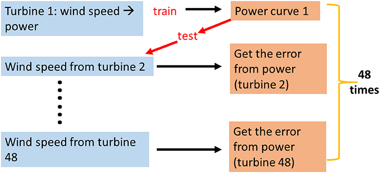
Figure 1. An outline of the steps for the offshore wind farm PBSHM. For each of the 48 wind turbines, a Gaussian process was trained to represent the individual power curve; this could then be used to predict power for all other turbines.

Figure 2 shows the average MSE errors represented in a form of confusion matrix. The figure shows how well each trained (reference) power curve predicts the power produced in the rest of the turbines on average, and also how well the power produced in each turbine is predicted by the rest of the trained curves (corresponding to the rest of the turbines). The y-axis of the confusion matrix shown in Figure 2 corresponds the index (1–48) of the training turbine and the x-axis to the index of the tested turbine. In general, with the normalization of the error adopted here, an MSE error below 5 is considered to show a good fit and below 1 would be considered excellent.

FIGURE 2

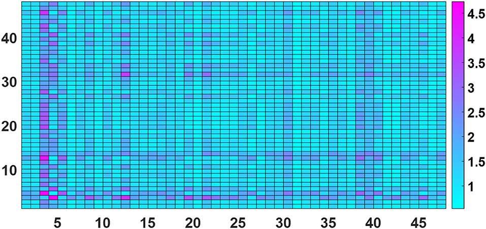
Figure 2. Confusion matrix of mean-square errors (MSEs) created from the GPs: testing set. The MSE is normalized here such that, if the mean of the training data is used as a minimal model, the value of the MSE is 100, and can be interpreted as a percentage. Any value less than 100% thus represents captured correlation.

The results of the paper showed that nearly all the models were very robust, with the highest MSE error occurring when the model trained on Turbine 4 was predicting power from Turbine 3. Both Turbines 3 and 4 are located in the outside row of the wind farm. However, the paper was limited in terms of SHM, as it was more of a performance monitoring study and many of the concepts described in earlier sections of this paper were not addressed in this work. A much more sophisticated framework for PBSHM is outlined in the next section; foundations that form the basis for a state-of-art conceptualization and implementation of PBSHM.

5. A General Framework for PBSHM

This section will now focus on newer developments in PBSHM, which to the authors' knowledge are the first serious attempt to form a general theoretical and computational framework for the problem. The basic concepts in the framework will be summarized here in a compact and comprehensive manner. Following the first steps discussed in the last section, many of the ideas were published in Bull et al. (2020b), Gosliga et al. (2020b), Gosliga et al. (2020c), Gardner and Worden (2020), Worden (2020), and Lin et al. (2020), and were then consolidated into (Bull et al., 2020a; Gardner et al., 2020a; Gosliga et al., 2020a).

5.1. Homogeneous Populations

The first step, as outlined before, in approaching PBSHM is to address the homogeneous population case, which is the simplest one, in which all members of the population can be considered to be nominally-identical; e.g., wind turbines within a wind farm. To approach the problem, a general model—called a form)—is employed to represent the overall behavior of the entire group, and can then be used to infer the presence of anomalous variations in individual members.

In general terms, the form is some model (or unified functional representation) that can be used to signify a homogeneous population of structures or systems. The model must thus capture the “essential” nature of the structure, but also represent the extent and nature of any variations between the members of the population, like manufacturing variations or other differences in embodiment. Machine learning is used to learn the form from some subset of the population; the training data are acquired from this subset when it is known to be in its undamaged conditions. Future (test) measurements can be assessed via the form, and then the robust generalized population model can be used for novelty detection across the entire population to check the condition of each structure. The point is that normality is assessed not only in terms of the variability of feature data from an individual structure, but also in terms of the likely variations across the population. An appropriate regression tool for establishing the form, is the previously mentioned Gaussian Process (Rasmussen and Williams, 2005; Murphy, 2012). The predictive mean of the GP is assumed to capture the “essence” of the structure, while the predictive variance provides a characterization of the variability across the population.

In order to demonstrate the power of the form concept, an example shall be given; for more complete definitions and more challenging examples of use, the reader is referred to Bull et al. (2020a). In this case study, a homogeneous population of 19 structurally-equivalent (8-DOF) systems was simulated, leading to a population of 19 members. Each individual is a model realization of an experimental rig, designed and constructed at the Los Alamos National laboratory (Bull et al., 2020a). The structure of interest is formed from eight very substantial masses connected by helical springs (Figure 3); it is as close to a lumped-mass system as one can construct, so the model division into eight masses and nine joints (springs) is entirely natural. The test-rig itself acts as the 20th member in the group, such that the total population is of 20 systems. The damage-sensitive features chosen to represent the system were Frequency Response Functions (FRFs). In order to construct the form, FRFs were estimated from the first ten members of the population; the resulting form is represented in Figure 4. The damage cases were simulated by reducing the stiffness of one of the springs in the structure, with three levels of severity; however, only the most severe case was represented in the experimental data. Again, for more details, the reader is referred to Bull et al. (2020a).

FIGURE 3

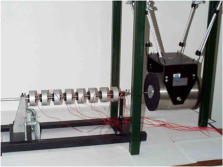
Figure 3. Eight degree-of-freedom experimental rig which is the basis of the form case study here.

FIGURE 4

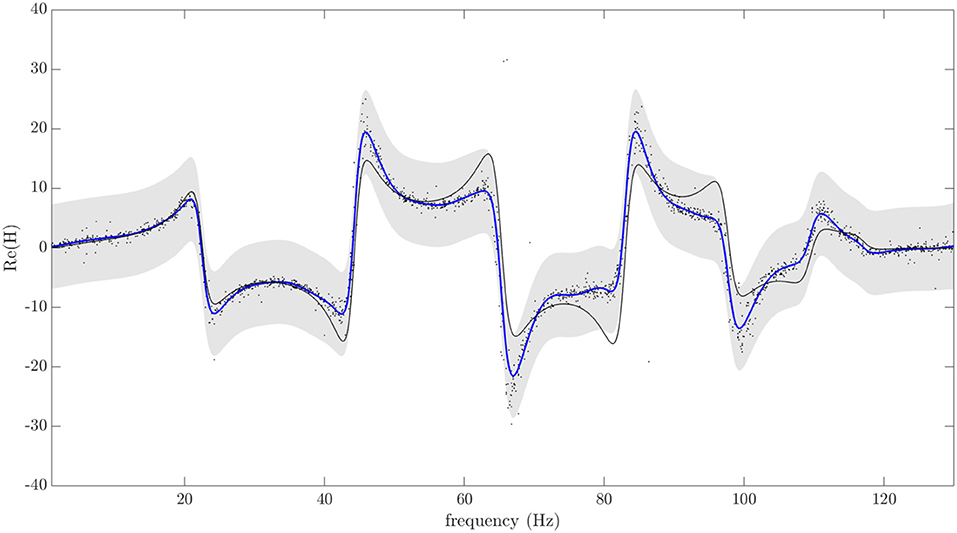
Figure 4. Gaussian process regression of the FRF as the population-form. Black markers indicate the training-set. The blue line indicates the posterior predictive mean and the shaded area indicates a 3-σ credible region, corresponding to the variance. The black line plots the mean function of the GP prior.

In order to test the form, the FRFs from the remaining ten members of the population were compared using a multivariate outlier statistic—the Mahalanobis squared-distance (MSD) (it is important to note that the covariance matrix for the MSD is not a sample estimate as in standard SHM outlier analysis (Worden et al., 1999), but is the full covariance matrix from the Gaussian process form). The results, as shown in Figure 5, are good; there are a minimum of false positives on the normal condition data; however, the variations across the population do tend to mask the lowest level of damage. This latter observation is going to be in the nature of PBSHM generally; variations across a population will tend to reduce sensitivity to damage. The answer to this problem is to adopt a strategy similar to data normalization for confounding influences; one needs to select appropriate features or to project out population variations, and this is a matter for further research. In this particular case, matters are not helped by the fact that natural frequencies are not always the most damage-sensitive features; they have been chosen here to facilitate comparison with previous work on this experimental system. On a positive note, the highest levels of damage are always detected, even for the experimental structure which was not included in the training set.

FIGURE 5

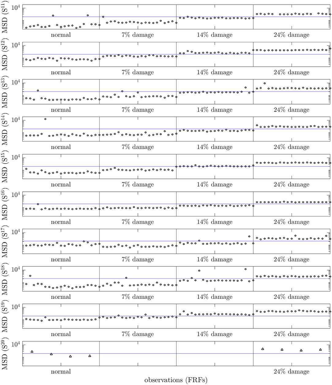
Figure 5. MSD novelty index for the test-data FRFs, comparing members 11–20. These members did not contribute training data to learn the form. The dot markers are used for simulated members 11–19, while triangle markers are used for the test-rig, member 20.

5.2. Heterogeneous Populations

The paper now considers the more challenging general case of heterogeneous populations of non-identical structures. The main machine learning tool that will be applied to this difficult task is transfer learning. Before describing an example that shows the benefits of transfer learning to PBSHM, some matters will first be clarified.

Firstly, it is important to confront the “myth” that one cannot utilize machine learning for SHM problems like localization, or classification of damage unless one always has millions of labeled examples for supervised learning. To dispel this idea, the reader is referred to Bull et al. (2019) and Bull et al. (2020c), where techniques like active and semi-supervised learning are demonstrated on SHM problems. This is an important point, because one of the major problems for SHM is the scarcity of labeled data. The fortunate reality is that one can learn useful representations from unlabeled data, domains or distributions with regard to heterogeneous populations, and can either train nearby surrogate objectives (where it is easier to generate matching label spaces), or use transfer learning to produce representations from related or even largely-unrelated tasks (Pan and Yang, 2009; Pan et al., 2010; Long et al., 2013; Wang et al., 2019; Gardner et al., 2020a,b).

Transfer learning provides the ability to utilize existing knowledge from a source task, in order to improve knowledge on/of a target task. The application to PBSHM is clear; where the source task is an SHM problem for a structure where data exist, and the target task is another structure where data are incomplete or absent. However, before attempting transfer, some important questions need to be addressed.

What to transfer: This is the most important question in the whole process. The engineer and learner seek to identify which part of the knowledge can be or should be transferred from the source to the target in order to improve the performance of the target task. It is important to identify which part of the knowledge is source-specific and which is likely to be common between the source and the target.

When to transfer: This is another critical question (which will be answered later through graph theory), as there are scenarios where transferring knowledge may make learning and SHM diagnostics worse rather than better (a phenomenon known as negative transfer). One must aim in SHM at utilizing transfer learning to improve target task performance and not simply to make a “tower of Babel” of learning outcomes that degrade the performance.

How to transfer: Once the previous questions are answered satisfactorily, one can proceed toward choice of algorithms that can actually transfer knowledge across domains/tasks. There are different transfer learning strategies and techniques for SHM purposes; the ones discussed here are mainly based on the idea of domain adoption.

Domain adaptation is one form of transfer learning that seeks to transfer feature spaces between source and target domains, assuming that their marginal distributions over source and task feature spaces are not equal (and often that the joint distributions between features and labels are different). One approach that is used, and will be the one illustrated here, is Joint Domain Adaption (JDA) (Pan and Yang, 2009; Pan et al., 2010; Long et al., 2013; Wang et al., 2019; Gardner et al., 2020a,b). A number of other algorithms are applicable to SHM algorithms, and some of the others are illustrated in Gardner et al. (2020b) and Gardner et al. (2020a). JDA is one of the techniques that assumes the joint distributions between feature and label spaces are different; it works by mapping the source and target features into a latent space where the distributions of data are harmonized. Harmony is enforced by minimizing the empirical form of the Maximum Mean Discrepancy (MMD) distance between the two distributions; this is the difference between two mean embeddings in a Reproducing Kernel Hilbert Space (RKHS).

The heterogeneous population case study used for illustration here, considers a population with geometry and material differences where the label spaces between the source and target domain are consistent (i.e., there are the same types of damage to classify). The two structures in the population here are both models of five-story shear structures (5-MDOF) with material differences (the first structure is steel and the other is aluminum), and with some geometric dissimilarities due to differences in the dimensions of the structures. The SHM problem is a six-class location problem where the damage scenarios are simulated for each of the degrees-of-freedom by simulating open cracks in the column members between floors. There are six labeled scenarios in total: one undamaged state and five damage states where damage is introduced between floors. The features for transfer are the five natural frequencies of the structures; because of the material and geometrical differences between the structures, their natural frequencies are quite different.

Figure 6 shows projections of the source and target domain features; the magnitudes of the natural frequencies are indeed very different, highlighting the need for transfer learning. Figure 7 shows projections of the identified transfer components from the JDA mapping into the latent space; the mapping has grouped the source and target domain clusters correctly together. Figures 6, 7 adopt a standard (and simple) strategy for visualizing data in high-dimensional spaces; the sub-figure at position (i, j) in the array shows a plot of variable i against variable j; the diagonal figures in the array (i, i) show the estimated densities (histograms) for the ith variable. Although this strategy is not perfect, one is limited by human physiology.

FIGURE 6

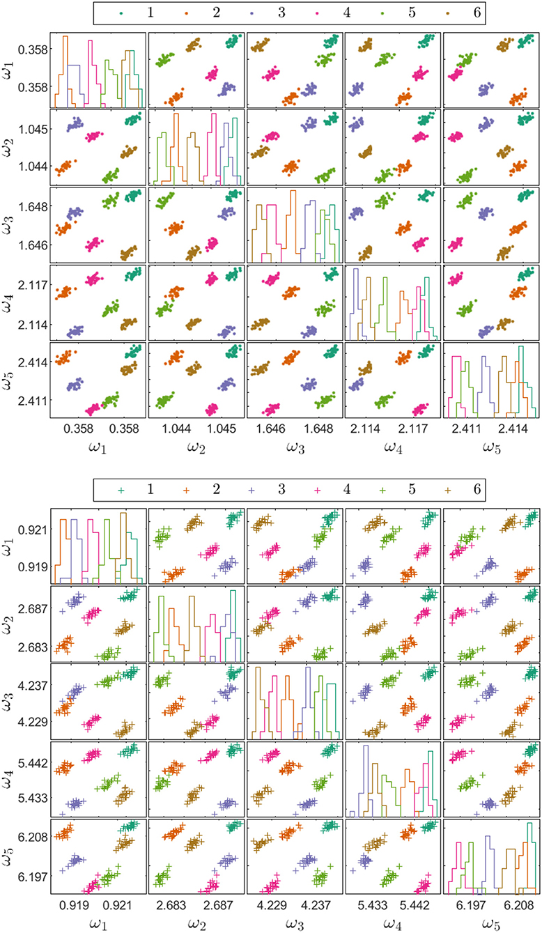
Figure 6. Source and Target domain features for the heterogeneous population case study with geometric and material differences (where damped natural frequencies are in Hz).

FIGURE 7

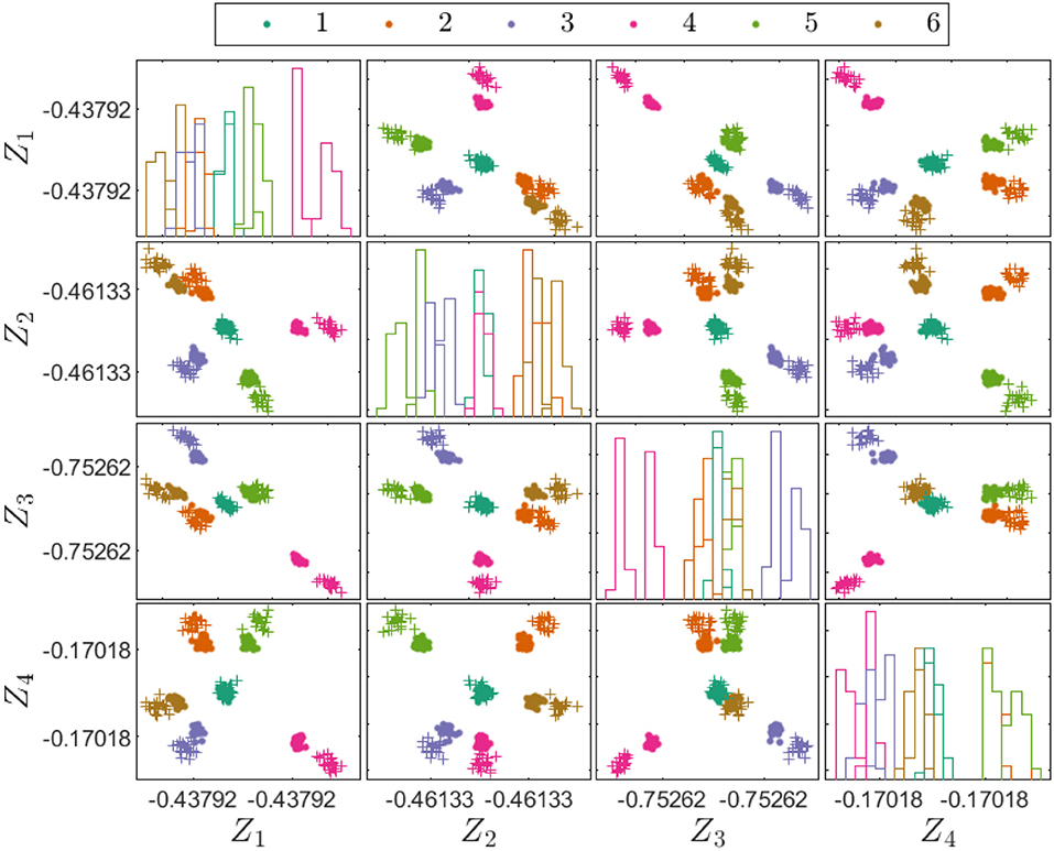
Figure 7. Transfer components for the source and target domains in the heterogeneous population case study with geometric and material differences. The source domain transfer components are denoted by dot markers, the target-domain training and testing transfer components are denoted by cross-markers and circle markets respectively.

A classifier in the latent space which correctly separates the source data, will also correctly identify the target data. In this case, a simple k-NN classifier was used, and the results are summarized in Table 1. Training on the source data and directly applying the classifier to the target gave results no better than random guessing, while JDA produced a perfect classification.

TABLE 1

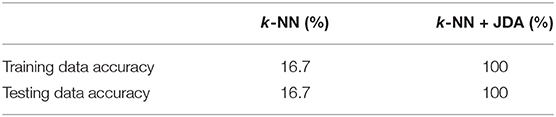
Table 1. Classification results for the heterogeneous population case study with geometric and material differences, trained on the labeled source domain and applied to unlabeled target domain (Gardner et al., 2020a,b).

5.3. Irreducible Elements and Attributed Graphs

As demonstrated, transfer learning has immense potential for SHM tasks. However, there are certain important issues related to transfer learning that need more careful exploration; in particular, it is critical to avoid negative transfer. One way to avoid this problem is to only attempt transfer if the source and target tasks are similar to each other; one way to achieve this for PBSHM is to try and ensure that the structures of interest are sufficiently similar in some sense. The question is then: how does one measure the similarity of structures? One way to do this would be to abstract a representation of structures that could be embodied in a metric space of some sort; the metric would then provide the required measure of similarity. For this reason, the PBSHM framework presented here is based on an abstract representation theory for structures. The metric space needed is constructed via two stages: in the first, irreducible element (IE) models of the structures are constructed; in the second stage, the IE models are converted to attributed graphs (AGs). As the space of attributed graphs is a metric space, it provides the desired comparison measure between structures.

In order to create an irreducible element (IE) model, the structure of interest is decomposed into components which have a well-established dynamic behavior e.g., beams, plates and shells. The model is not designed for dynamic prediction, but rather to identify the essential elements that define the nature of the structure. The process is illustrated in Figure 8. The representation associates a parameter vector with each IE, which stores the material properties and dimensions of the IE. The process is described in much more detail in Gosliga et al. (2020a)

FIGURE 8

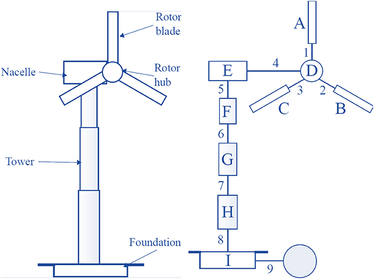
Figure 8. An expanded IE representation of a wind turbine with the elements labeled A to I and the connections labeled 1–9. The shaded node is a special element representing the ground, where the boundary condition is defined in the attributes for Joint 9.

The IE model is then converted into the attributed graph (AG) model. This step is carried out by associating a graph node with each IE; the parameter vector from the IE is attached to the node, thus creating an attributed graph. If two IEs are connected in the structure, the two corresponding AG nodes are joined by an edge; the edge will also carry attributes i.e., a parameter vector specifying the type and parametric description of the joint. The IE model and the AG are thus in one-to-one correspondence. Because of this, the metric on the space of AGs carries over to the “space” of IE models and provides a measure of similarity between structures. This measure can then be used to inform the level of inference that can (potentially) be made between structures within a population. This framework also allows a precise definition of population types as follows. One defines two structures to be topologically equivalent if their induced AGs are topologically equivalent i.e., have the same number of nodes and corresponding edges in place. As the boundary conditions for a structure are critical, connections to ground are represented by a special node—the ground node—and boundary conditions are encoded in the edge attributes for nodes connecting to ground. Two structures are deemed structurally equivalent if their corresponding AGs are topologically equivalent and the ground nodes in the two graphs are in correspondence. Figure 9 illustrates some AG representations which are, and are not, structurally equivalent. A simple definition of a homogeneous population is then one that is composed of structures which are pairwise structurally equivalent; however, things are a little more complicated than this in general, and the details can be found in Gosliga et al. (2020a). A heterogeneous population is then simply one that is not homogeneous.

FIGURE 9

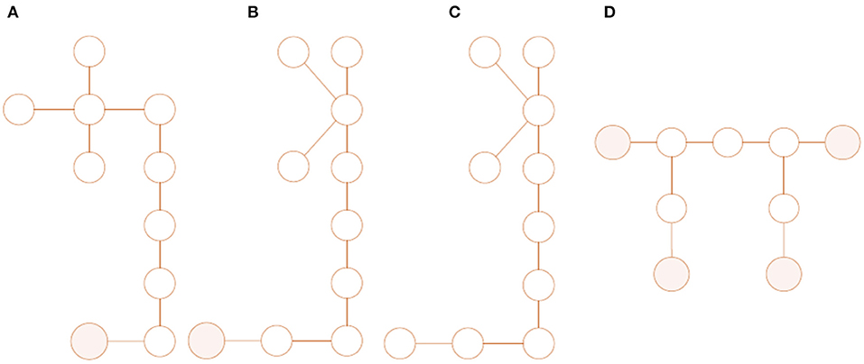
Figure 9. Graphical representations of structures, ground nodes are shaded. (A,B): Two topologically-equivalent graphs, used to represent structurally-equivalent wind turbines, that have simply been drawn differently. (C): A graph that is topologically equivalent to (A,B) but not structurally, due to inconsistency in ground nodes. (D) a graph used to represent a three-span bridge, that is topologically and structurally inequivalent to (A–C).

The question remains as to how to specify the metric on the space of AGs; one way to do this is via the maximum common subgraph (MCS). Two graphs are clearly more similar if they have more common structure, and this captured in the size of their MCS. Furthermore, the MCS makes sense from a PBSHM point of view; common subgraphs in the AG correspond to common substructures in the structures of interest. If an SHM problem is to be transferred between structures, the process is clearly more likely to succeed if the problem occurs within a common substructure. The process of extracting the MCS between two graphs is computationally demanding; the algorithm used for the illustration here is the Bron-Kerbosch algorithm as described in Gosliga et al. (2020a). Once the MCS is established, this can be converted into a metric distance which is smaller when two structures share larger MCSs; the metric used here and described in Gosliga et al. (2020a), is the Jaccard similarity coefficient. Figure 10 shows two AGs associated with a wind turbine and an airplane; although these look quite different, they do possess an extended common subgraph, which is shown in Figure 11. The subgraph corresponds to the chain (and branches) running from A to H in the wind turbine graph and that running from M to F in the airplane graph; in fact there are multiple chains from M that have the same subgraph structure.

FIGURE 10

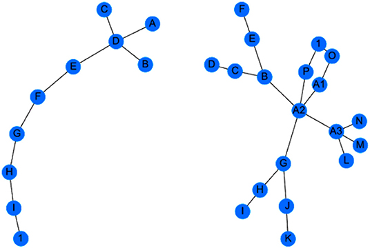
Figure 10. Graph models for two structures: a wind turbine (left) and an airplane (right).

FIGURE 11

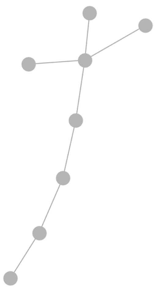
Figure 11. Maximum common subgraph between the two AG models illustrated in Figure 10.

Figure 12 tries to summarize the main concepts of PBSHM via a flowchart, from homogeneous populations to heterogeneous populations and from forms, and transfer learning to graph theory integration. Throughout this paper, the main emphasis has been on expressing the basic ideas of the proposed population-based framework. Because of the limitations of space, this approach has inevitably lacked detail in terms of the case study structures and their experimental investigation. The curious reader is again directed toward the foundational papers for the missing detail: (Bull et al., 2020a; Gardner et al., 2020a; Gosliga et al., 2020a).

FIGURE 12

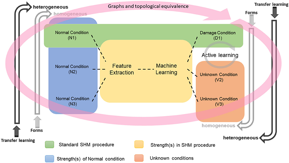
Figure 12. Population-based SHM summary.

6. Conclusions

Population-based SHM (PBSHM) offers significant advantages for the research field and also in terms of the implementation of SHM in an industrial environment, as it can address problems like label deficiency, structural performance, data minimization and robust performance metrics as well as validation and verification of SHM systems. Valuable information can be transferred between groups of similar or dissimilar structures. Knowledge transfer and mapping are critical processes in developing PBSHM such that inferences about health states can be transferred. It was stressed here, how important it is when applying transfer learning to determine what similarities exist between structures within a population, and what information could and should be transferred, such that negative transfer is avoided. In order to characterize similarities between structures an abstract representation theory has been described, based on attributed graph (AG) representations via irreducible element (IE) models. In the case of homogeneous populations (of nominally-identical structures), the concept of the form was discussed as a powerful tool for PBSHM. For more general heterogeneous populations, examples of transfer learning were presented and discussed.

This paper summarizes foundations for a theory and methodology for population-based SHM, in order to perform knowledge transfer within and between homogeneous and heterogeneous populations. The integration of an IE and AG-based approach to quantify knowledge about structures is vital in understanding the effectiveness of PBSHM architectures.

Author Contributions

KW, LB, PG, JG, TR, EC, EP, WL, and ND: conceptualization, methodology, software, writing, review, and editing.

Conflict of Interest

The authors declare that the research was conducted in the absence of any commercial or financial relationships that could be construed as a potential conflict of interest.

Acknowledgments

The authors gratefully acknowledge the support of the UK Engineering and Physical Sciences Research Council (EPSRC) through grant references EP/R003645/1, EP/R004900/1, EP/S001565/1, and EP/R006768/1. They would also like to thank Dr. Eoghan Maguire of Vattenfall, for providing access to the Lillegrund data.

References

Bull, L., Gardner, P., Gosliga, J., Dervilis, N., Papatheou, E., Maguire, A. E., et al. (2020a). Foundations of population based structural health monitoring, part I: homogeneous populations and forms. Mech. Syst. Signal Process. 148:107141. doi: 10.1016/j.ymssp.2020.107141

CrossRef Full Text | Google Scholar

Bull, L., Gardner, P., Gosliga, J., Maguire, A., Campos, C., Rogers, T., et al. (2020b). “Towards population-based structural health monitoring, Part I: homogeneous populations and forms,” in Proceedings of IMAC XXXVIII-the 38th International Modal Analysis Conference (Houston, TX).

Bull, L., Rogers, T., Wickramarachchi, C., Cross, E., Worden, K., and Dervilis, N. (2019). Probabilistic active learning: an online framework for structural health monitoring. Mech. Syst. Signal Process. 134:106294. doi: 10.1016/j.ymssp.2019.106294

CrossRef Full Text | Google Scholar

Bull, L., Worden, K., and Dervilis, N. (2020c). Towards semi-supervised and probabilistic classification in structural health monitoring. Mech. Syst. Signal Process. 140:106653. doi: 10.1016/j.ymssp.2020.106653

CrossRef Full Text | Google Scholar

Deering, S., Manson, G., Worden, K., Allen, D., Farrar, C., and Lombardo, J. (2008). “Syndromic surveillance as a paradigm for SHM data fusion,” in Proceedings of 4th European Workshop on Structural Health Monitoring (Krakow).

Google Scholar

Farrar, C., and Worden, K. (2012). Structural Health Monitoring: A Machine Learning Perspective. John Wiley and Sons. doi: 10.1002/9781118443118

CrossRef Full Text | Google Scholar

Gardner, P., Bull, L., Gosliga, J., Dervilis, N., and Worden, K. (2020a). Foundations of population-based structural health monitoring, part III: heterogeneous populations-transfer and mapping. Mech. Syst. Signal Process. 149:107142. doi: 10.1016/j.ymssp.2020.107142

CrossRef Full Text | Google Scholar

Gardner, P., Liu, X., and Worden, K. (2020b). On the application of domain adaptation in structural health monitoring. Mech. Syst. Signal Process. 138:106550. doi: 10.1016/j.ymssp.2019.106550

CrossRef Full Text | Google Scholar

Gardner, P., and Worden, K. (2020). “Towards population-based structural health monitoring, Part IV: Heterogeneous populations, matching and transfer,” in Proceedings of IMAC XXXVIII-the 38th International Modal Analysis Conference (Houston, TX).

Gosliga, J., Gardner, P., Bull, L., Dervilis, N., and Worden, K. (2020a). Foundations of population-based structural health monitoring, part II: heterogeneous populations-graphs, networks and communities. Mech. Syst. Signal Process. 148:107144. doi: 10.1016/j.ymssp.2020.107144

CrossRef Full Text | Google Scholar

Gosliga, J., Gardner, P., Bull, L., Dervilis, N., and Worden, K. (2020b). “Towards population-based structural health monitoring, Part II: heterogeneous populations and structures as graphs,” in Proceedings of IMAC XXXVIII-the 38th International Modal Analysis Conference (Houston, TX).

Google Scholar

Gosliga, J., Gardner, P., Bull, L., Dervilis, N., and Worden, K. (2020c). “Towards population-based structural health monitoring, Part III: graphs, networks and communities,” in Proceedings of IMAC XXXVIII-the 38th International Modal Analysis Conference (Houston, TX).

Google Scholar

Hensman, J., Worden, K., Eaton, M., Pullin, R., Holford, K., and Evans, S. (2011). Spatial scanning for anomaly detection in acoustic emission testing of an aerospace structure. Mech. Syst. Signal Process. 25, 2462–2474. doi: 10.1016/j.ymssp.2011.02.016

CrossRef Full Text | Google Scholar

Lin, W., Worden, K., Maguire, A., and Cross, E. (2020). “Towards population-based structural health monitoring, Part VII: EoV fields: environmental mapping,” in Proceedings of IMAC XXXVIII-the 38th International Modal Analysis Conference (Houston, TX).

Google Scholar

Long, M., Wang, J., Ding, G., Sun, J., and Yu, P. (2013). “Transfer feature learning with joint distribution adaptation,” in Proceedings of the IEEE International Conference on Computer Vision (Sydney, NSW), 2200–2207. doi: 10.1109/ICCV.2013.274

CrossRef Full Text | Google Scholar

Murphy, K. (2012). Machine Learning: A Probabilistic Perspective. MIT Press.

Google Scholar

Pan, S., Tsang, I., Kwok, J., and Yang, Q. (2010). Domain adaptation via transfer component analysis. IEEE Trans. Neural Netw. 22, 199–210. doi: 10.1109/TNN.2010.2091281

PubMed Abstract | CrossRef Full Text | Google Scholar

Pan, S., and Yang, Q. (2009). A survey on transfer learning. IEEE Trans. Knowledge Data Eng. 22, 1345–1359. doi: 10.1109/TKDE.2009.191

CrossRef Full Text | Google Scholar

Papatheou, E., Dervilis, N., Maguire, A., Antoniadou, I., and Worden, K. (2014). “Population-based SHM: a case study on an offshore wind farm,” in Proceedings of 10th International Workshop on Structural Health Monitoring (Palo Alto, CA). doi: 10.12783/SHM2015/60

CrossRef Full Text | Google Scholar

Papatheou, E., Dervilis, N., Maguire, A., Antoniadou, I., and Worden, K. (2015). A performance monitoring approach for the novel Lillgrund offshore wind farm. IEEE Trans. Indus. Electron. 62, 6636–6644. doi: 10.1109/TIE.2015.2442212

CrossRef Full Text | Google Scholar

Papatheou, E., Dervilis, N., Maguire, A., Campos, C., Antoniadou, I., and Worden, K. (2017). Extreme function theory for SHM: an application to wind turbines. Renew. Energy 113, 1490–1502. doi: 10.1016/j.renene.2017.07.013

CrossRef Full Text

Rasmussen, C., and Williams, C. (2005). Gaussian Processes for Machine Learning. The MIT Press. doi: 10.7551/mitpress/3206.001.0001

CrossRef Full Text | Google Scholar

Sohn, H. (2007). Effects of environmental and operational variability on structural health monitoring. Philos. Trans. R. Soc. A 365, 539–560. doi: 10.1098/rsta.2006.1935

PubMed Abstract | CrossRef Full Text | Google Scholar

Tay, C., and Laugier, C. (2008). “Modelling smooth paths using Gaussian processes,” in Proceedings of the International Conference on Field and Service Robotics (Berlin; Heidelberg: Springer). doi: 10.1007/978-3-540-75404-6_36

CrossRef Full Text | Google Scholar

Vamvoudakis-Stefanou, K., and Fassois, S. (2017). Vibration-based damage detection for a population of nominally identical structures via random coefficient Gaussian mixture AR model based methodology. Proc. Eng. 199, 1888–1893. doi: 10.1016/j.proeng.2017.09.123

CrossRef Full Text | Google Scholar

Vamvoudakis-Stefanou, K., Sakellariou, J., and Fassois, S. (2014). “Random vibration response-only damage detection for a set of composite beams,” in Proceedings of the ISMA International Conference on Noise and Vibration.

Google Scholar

Vamvoudakis-Stefanou, K., Sakellariou, J., and Fassois, S. (2018). Vibration-based damage detection for a population of nominally identical structures: unsupervised multiple model (MM) statistical time series type methods. Mech. Syst. Signal Process. 111, 149–171. doi: 10.1016/j.ymssp.2018.03.054

CrossRef Full Text | Google Scholar

Wang, Z., Dai, Z., Póczos, B., and Carbonell, J. (2019). “Characterizing and avoiding negative transfer,” in Proceedings of the IEEE Conference on Computer Vision and Pattern Recognition (Long Beach, CA), 11293–11302. doi: 10.1109/CVPR.2019.01155

PubMed Abstract | CrossRef Full Text | Google Scholar

Worden, K. (2020). “Towards a population-based structural health monitoring. Part VI: structures as geometry,” in Proceedings of IMAC XXXVIII-the 38th International Modal Analysis Conference (Houston, TX).

Worden, K., Cross, E., Dervilis, N., Papatheou, E., and Antoniadou, I. (2015). Structural health monitoring: from structures to systems-of-systems. IFAC Papers Online 28, 1–17. doi: 10.1016/j.ifacol.2015.09.497

CrossRef Full Text | Google Scholar

Worden, K., Manson, G., and Fieller, N. (1999). Damage detection using outlier analysis. J. Sound Vibrat. 229, 647–667. doi: 10.1006/jsvi.1999.2514

CrossRef Full Text | Google Scholar