Quantifying Tidal Phase Effects on Coastal Flooding Induced by Hurricane Sandy in Manhattan, New York Using a Micro-Scale Hydrodynamic Model

Introduction

New York City (NYC) is among the top three cities in the world in terms of assets exposed to coastal flooding (Nicholls et al., 2007). NYC is highly vulnerable to coastal flooding as best exemplified by Hurricane Sandy in 2012. Sandy caused 43 fatalities and $19 billion in damages in NYC (City of New York, 2013). Hurricane Sandy generated the highest recorded water level in the NYC region since at least the past 300 years (Orton et al., 2019), with an estimated flood return period of between 260-year (Orton et al., 2016) and 398-year (Lin et al., 2016). The southern part of Manhattan was one of the areas in NYC that were hardly impacted by extreme water levels during Hurricane Sandy. At The Battery tide gauge station in Lower Manhattan (see Figure 1), Sandy generated a storm surge of 2.81 m above the mean sea level (Marsooli et al., 2017). The storm surge overtopped the seawalls of Lower Manhattan and flooded low-lying streets, tunnels, and subway stations.

FIGURE 1

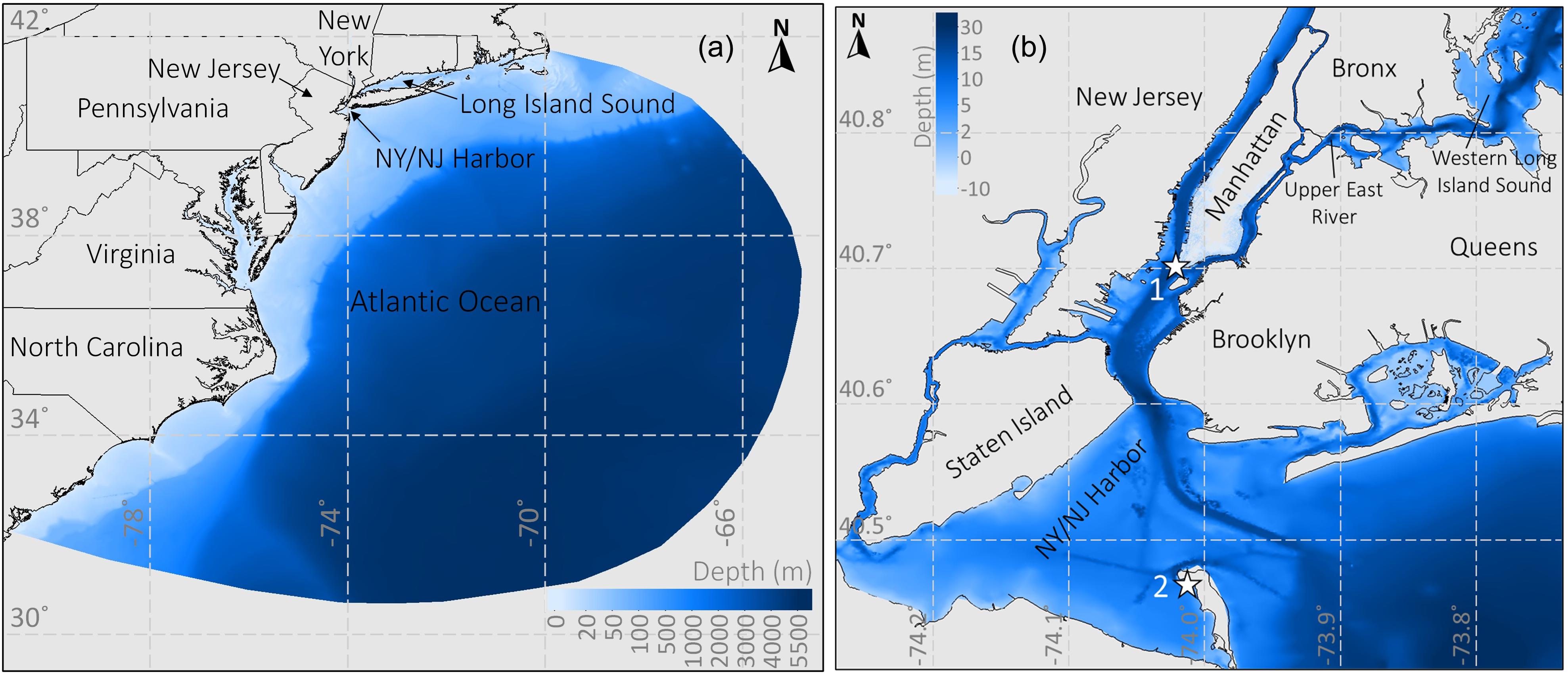
Figure 1. The extent and bathymetry of the computational domain in (a) Atlantic Ocean and (b) NY/NJ Harbor. Star signs labeled as 1 and 2 represent, respectively, the locations of The Battery and Sandy Hook tide gauge stations.

Hurricane Sandy’s peak storm surge in New York/New Jersey (NY/NJ) Harbor coincided nearly with the high tide. At the southern part of Manhattan (i.e., the location of The Battery station), the peak surge height arrived only 30 min after the normal astronomical high tide. On the other hand, at the eastern part of Manhattan (i.e., in the Upper East River and Western Long Island Sound), where the tidal range is greater than 1.5 m, the maximum surge height coincided nearly at the time of the local normal low tide. Georgas et al. (2014) found that the flood level along the Upper East River and Western Long Island Sound could be up to 0.9–1.2 m higher if Sandy happened to have come ashore 7–10 h earlier. The substantial effect of the tidal phase on the water level raises the question that what the extent and depth of coastal flooding in NYC would have been if Sandy had arrived several hours earlier.

Compound flooding due to astronomical tides, storm surges, and river flows is a major hazard in low-lying coastal areas (Zhong et al., 2013; Sopelana et al., 2018; Bermúdez et al., 2019; Valle-Levinson et al., 2020). Bermúdez et al. (2019) showed that studies of flood hazards in coastal river reaches should account for the role of and interactions between coastal and inland flood drivers. In coastal regions with large tidal amplitudes, tides could substantially contribute to the total water level during a storm event, leading to compound flooding due to tides and storm surges. Non-linear tide-surge interactions also contribute to the storm-induced water levels (e.g., Lyddon et al., 2018; Marsooli and Lin, 2018).

Georgas et al. (2014) used a “bathtub” technique to predict the effects of tidal phase on the extent and depth of flooding in NYC. In the bathtub technique, the storm tide calculated in the coastal ocean is assumed to horizontally extent over land and inundate areas with an elevation equal to or lower than the calculated storm tide level. The bathtub technique neglects the effects of fluid dynamics on the propagation of floodwaters over land and, thus, the generated flood maps are independent of the flow momentum, bottom friction, wind, and other factors that govern the floodwater dynamic.

Hydrodynamic models are accurate tools to predict coastal flooding over land. Implementation of hydrodynamic models to simulate flooding in urban areas is a challenging task because of the presence of urban features such as roads and buildings which affect the fluid dynamics. Depending on the shape and size of individual buildings, roads can become narrow open channels during a coastal flood event. Depending on the bed slope, the floodwater speed in these channels could remain high for a considerable period of time due to a relatively small bottom friction of paved roads.

In the past studies of coastal flood simulation in urban areas using hydrodynamic models, different approaches have been adopted to represent buildings in the computational domain. The most common approach is the building-resistance method that increases the bottom friction (e.g., Manning’s coefficient) in computational nodes that are located within building footprints (e.g., Gallien et al., 2011; Takagi et al., 2016; Yin et al., 2016). In this approach, the floodwater can flow over areas occupied by buildings, which would adversely impact the simulated flood characteristics. Another approach, which is called building-block method, represents buildings by raising the bed elevation of computational nodes that are within building footprints. However, this approach would result in steep slopes in the model topography and consequently cause numerical instability. Some other approaches account for the effects of buildings through partial wetting and drying schemes, building-porosity, and cut-cell methods (e.g., An and Yu, 2012; Schubert and Sanders, 2012; Wang et al., 2014).

An accurate method to represent buildings in computational domains, which is called building-hole method, is to remove computational nodes that are within building footprints (e.g., Aronica et al., 1998; Schubert et al., 2008; Cea et al., 2010). For example, Blumberg et al. (2015) developed a “street-scale” finite difference Cartesian grid with rectangular cells to simulate coastal flooding induced by Hurricane Sandy in an urban area in New Jersey waterfronts. Representing buildings in Cartesian grids has its challenges. Removing rectangular cells results in a stepwise approximation of boundaries. The Stepwise approximation is not smooth and leads to errors near the boundaries. The errors can propagate into the whole domain during the simulation. A more accurate representation of buildings can be obtained by using hydrodynamic models that utilize flexible unstructured and body-fitted meshes that conform to any desired geometry. This approach is adopted in the present study to represent urban features in the computational domain of Manhattan.

The objective of the present study is to reveal the effects of tide timing on the extent and depth of coastal flooding induced by Hurricane Sandy in Manhattan. We obtain the study objective using a coupled circulation-wave model and by developing a micro-scale unstructured computational mesh that resolves urban features including roads, buildings, and seawalls in Manhattan. We validate the model using storm tides (i.e., total water levels) measured at tide gauge stations in NY/NJ Harbor and high-water marks collected in Manhattan. The model is then utilized to simulate a number of numerical experiments to investigate the effects of tides on the extent and depth of coastal flooding.

Materials and Methods

Hydrodynamic Model

We implement the two-dimensional version of ADvanced CIRCulation model (ADCIRC) coupled with the Simulating WAves Nearshore model (SWAN) (Dietrich et al., 2011) to simulate storm tide and coastal flooding in the study area. ADCIRC (Luettich et al., 1992; Westerink et al., 1994) is a high-fidelity finite-element coastal ocean circulation model that solves the depth-averaged continuity equation in Generalized Wave-Continuity Equation form to calculate the water surface level and the depth-averaged mean flow momentum equations to calculate the water flow velocity. SWAN (Booij et al., 1999; Ris et al., 1999) is a spectral wave model that solves the depth-averaged two-dimensional wave action balance equation to calculate the wave action density and the phase-averaged wave characteristics. Coupling the circulation and wave models allow to include the effects of surface waves on the total water level. Details on the governing equations and numerical methods can be found in the references cited above.

Computational Domain

We develop a micro-scale computational mesh that covers low-lying areas of Manhattan and extends to NY/NJ Harbor and the Atlantic Ocean (Figure 1). The computational mesh consists of 668,977 nodes and 1,253,688 elements. The mesh resolution is between 3 and 8 m in Manhattan (Figure 2), between 100 and 1,000 m in NY/NJ Harbor, and reaches about 25 km in the deep ocean. The mesh is generated using the OceanMesh2D program (Roberts and Pringle, 2018; Roberts et al., 2019) and quality-checked and manually trimmed using the SMS software (Aquaveo, 2013). The developed mesh is utilized as the geographical mesh in both ADCIRC and SWAN. The spectral mesh in SWAN consists of 36 directional bins, and the lowest and highest wave frequencies are set to 0.03 and 1 Hz, respectively.

FIGURE 2

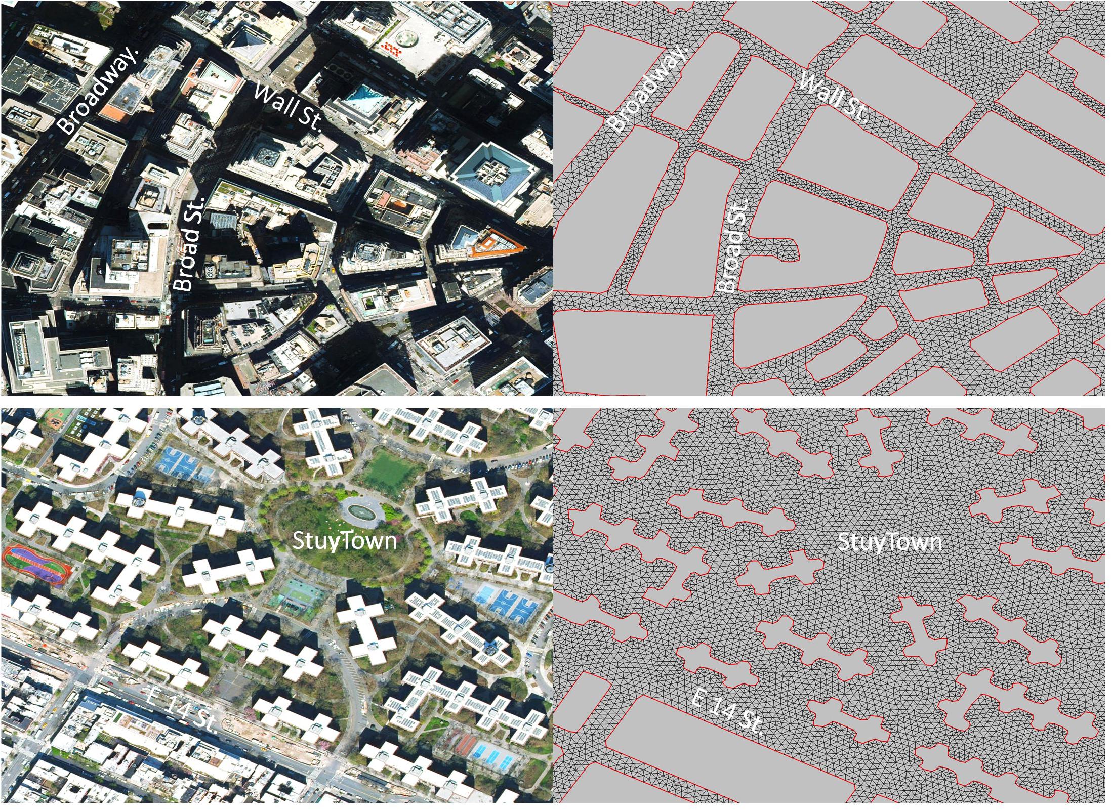
Figure 2. Computational mesh in Manhattan has a resolution of between 3 and 8 m and resolves urban features such as buildings and roads (top panel: a financial district in Lower Manhattan. bottom panel: a residential neighborhood on the east side of Manhattan, see Figure 3 for the locations). Left panels are based on World Imagery from Surface-water Modeling System, SMS, software (https://www.aquaveo.com/).

Buildings are represented in the mesh as island boundaries (see Figures 2, 3). Building footprints are based on the shapefile of 2016 footprint outlines of buildings in NYC (Department of Information Technology and Telecommunications, 2016). Seawalls around Manhattan are represented in the mesh as weirs, which are defined as internal boundaries in the ADCIRC model (based on the broad-crested weir formula). ADCIRC uses a basic weir formula to calculate the flow rate over the weir when the water level exceeds the weir height. We set the weir height to the elevation of shorelines in Manhattan, which is about 2.5 m above the mean sea level (Orton et al., 2019).

FIGURE 3

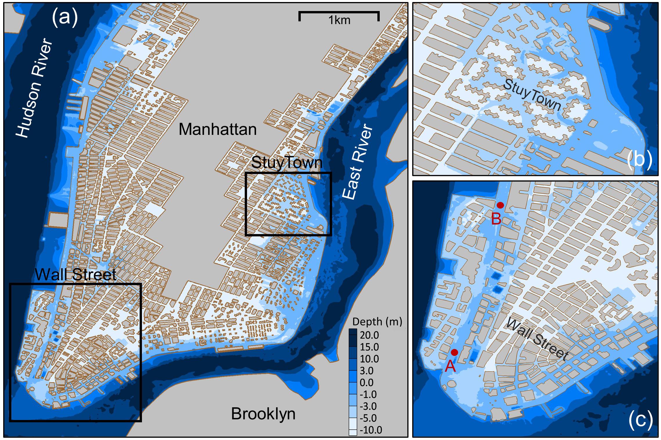
Figure 3. Computational domain in (a) Manhattan, (b) neighborhoods around StuyTown, and (c) Wall Street. The domain extends to an elevation of about 10 m above mean sea level. Points A and B are the locations of model outputs that are discussed later.

The topographic data are based on the NYC 1foot (about 0.3 m) Digital Elevation Model, which is a bare-earth digital-elevation surface model derived from 2010 Light Detection and Ranging data (Department of Information Technology and Telecommunications, 2013). The bathymetry data in NY/NJ Harbor are from the Continuously Updated Digital Elevation Model (CUDEM) with a spatial resolution of 1/9 Arc-Second (about 3.4 m) (Cooperative Institute for Research in Environmental Sciences, 2014). Outside NY/NJ Harbor, the bathymetry is from Shuttle Radar Topography Mission (SRTM), version SRTM15 + V2 (Tozer et al., 2019), which is a global dataset with a resolution of 15 Arc Second (about 500 m). The bottom friction coefficient is specified based on the land cover type from the 3 ft (about 9.1 m) landcover dataset of NYC. We set the Manning’s roughness coefficient to 0.017 s.m^–1/3 for open waters, 0.022 s.m^–1/3 for roads and paved surfaces, 0.03 s.m^–1/3 for bare soil, and 0.035 s.m^–1/3 for vegetated land (coefficients were selected based on sensitivity analysis and the range of recommended values in the literature).

Tidal and Meteorological Forcing

Tidal forcing in the model is specified based on eight major tidal constituents K1, K2, M2, N2, O1, P1, Q1, and S2. Tidal data, including amplitudes and phases, are obtained from the global model of ocean tides TPXO8–ATLAS with a 1/30° resolution (Egbert and Erofeeva, 2002). Meteorological forcing is based on the reanalysis data from the Oceanweather Inc.¹ Wind data are generated for open-ocean marine conditions without considering the effects of roughness elements on land. We implement the ADCIRC’s directional land-masking approach (Westerink et al., 2008; Bunya et al., 2010) to adjust the wind speed based on the land type and the presence of roughness elements such as buildings and trees.

Numerical Experiments

We perform a series of numerical experiments to investigate the effects of tide timing on the coastal flooding in the study area. The experiments consider the peak surge height arrives at different tidal phases during a full tidal cycle (Figure 4). Experiments include a control run (actual storm surge arrival time), and 2, 4, 6, 8, 10, and 12 h early experiments. The 2–12 h early experiments consider that Hurricane Sandy made landfall 2–12 h earlier than its actual time of landfall. All simulations last for 8.6 days (with the start date of the control run in October 22, 1800ETS).

FIGURE 4

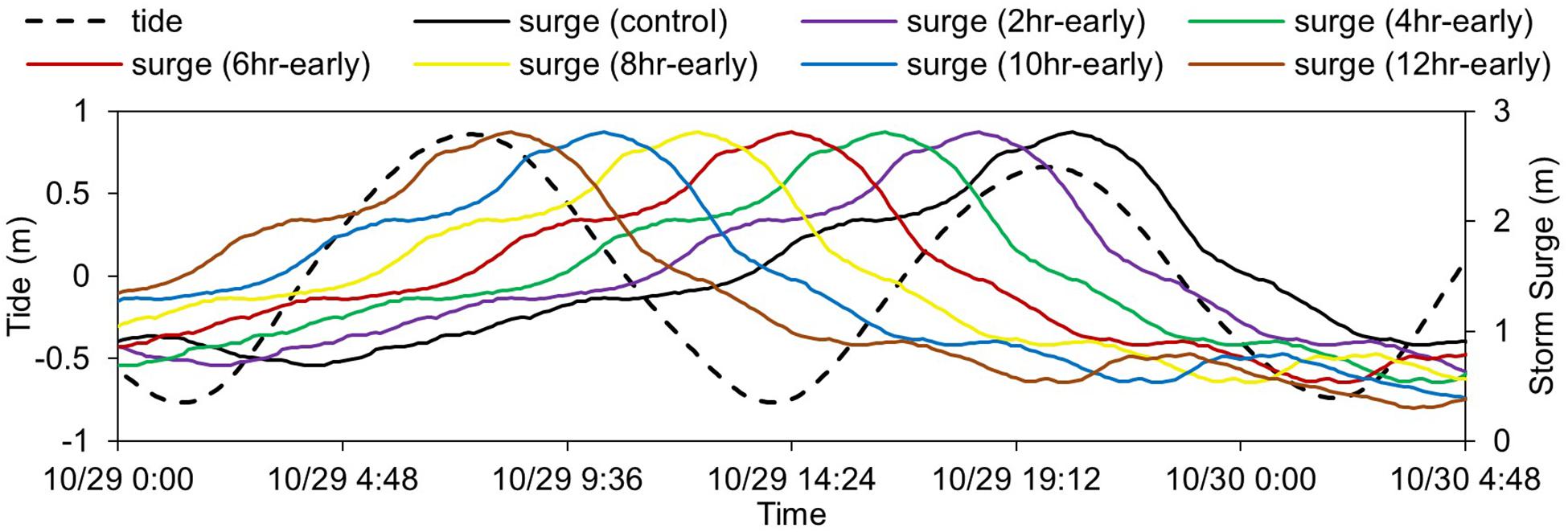
Figure 4. Time series of tides and storm surge heights at different arrival times considered in the numerical experiments.

Model Evaluation

Using water level observations during Hurricane Sandy, we evaluate the accuracy of the developed flood model to simulate storm tides in NY/NJ Harbor and coastal flooding in Manhattan. Hurricane Sandy was a Category 3 storm at its peak intensity and went through an extratropical transition a few hours before making landfall on the East Coast of the United States. At 2330 UTC on October 29, 2012 Sandy made landfall near Brigantine, New Jersey as an extratropical cyclone. According to data from a variety of observational platforms, Sandy was the largest tropical cyclone since 1988, with an extent (diameter) of destructive winds of about 1600 km prior to the landfall. Because of its size, Sandy generated catastrophic storm surges and waves that severely flooded coastal areas of New Jersey and New York. It caused at least $50 billion in damage in the United States, and 72 deaths in the mid-Atlantic and northeastern United States (Blake et al., 2013).

Figure 5 compares modeled and measured time series of storm tide (total water level) and storm surge at The Battery and Sandy Hook tide gauge stations (see Figure 1 for the location of the tide gauge stations). The model captures the arrival time, duration, and peak storm tides and surges. The storm surge height before the arrival of the peak surge is slightly underestimated, which can be due to the forerunner surges that are not captured by the model. To simulate forerunners, the computational domain should cover a larger area in the ocean or be nested in a basin-scale model. Storm surge time series also show a slight time lag between the modeled and measured falling surge height, which can be because of river discharge from Hudson River and three-dimensional flows that are neglected in this study. Nevertheless, the model shows a high accuracy to simulate coastal flooding in Manhattan. Figure 6 shows that the model reproduces well the measured high-water marks (Schubert et al., 2015). The modeled high-water marks have a root-mean-square-error of 15 cm and a bias of 7 cm.

FIGURE 5

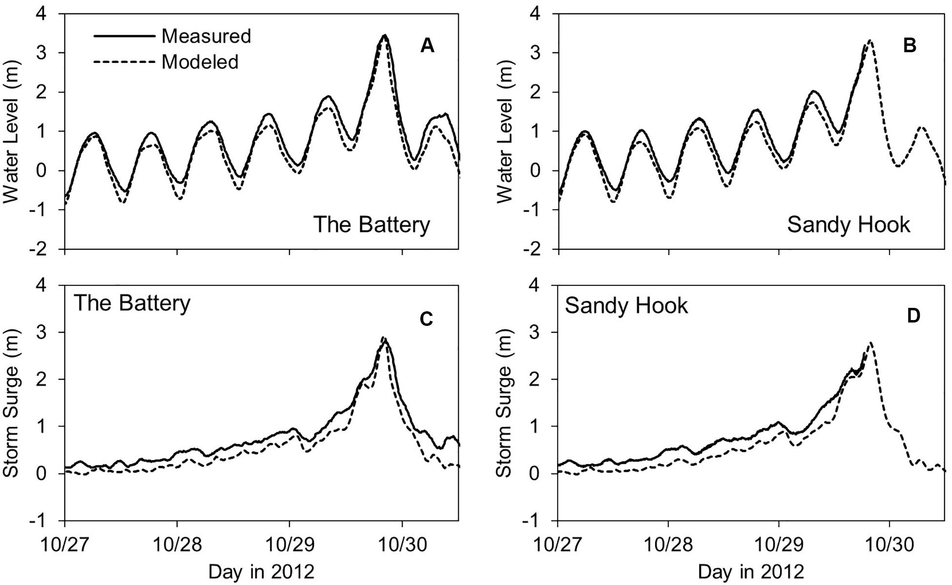
Figure 5. Measured and modeled time series of storm tide (water level) and storm surge at (A,C) The Battery and (B,D) Sandy Hook tide gauge stations. The vertical datum is in mean sea level.

FIGURE 6

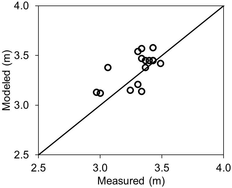
Figure 6. Measured and modeled high-water marks in Manhattan.

Modeled spatial distribution of coastal flooding (Figure 7) illustrates a wider extent of flooding in neighborhoods on the east side of Manhattan along the East River. The flood depth is larger in the southern and eastern sides of the study area and locally surpasses 2 m in some neighborhoods. The results are consistent with previous studies (e.g., Yin et al., 2016).

FIGURE 7

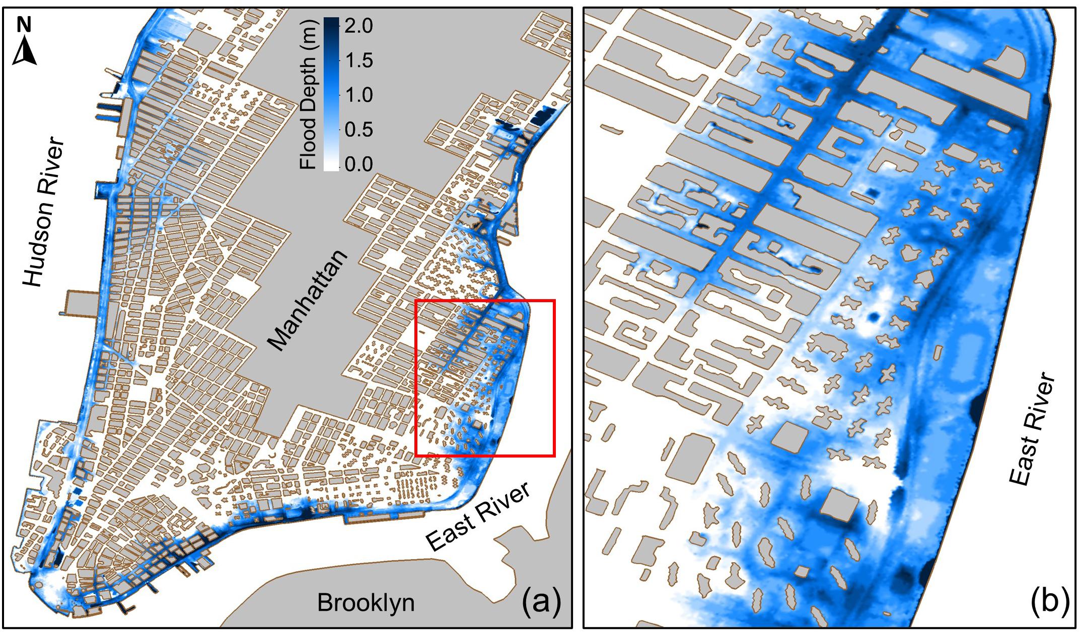
Figure 7. Modeled spatial distribution of maximum flood depth in Manhattan during Hurricane Sandy in (a) the study area and (b) a neighborhood on the east side of Manhattan.

Results and Discussion

Numerical experiments reveal that the tide timing has a significant impact on the storm tide off the shoreline and the extent and depth of coastal flooding in the study area. The storm tide level at The Battery tide gauge station would be larger than the observed storm tide level if Hurricane Sandy arrives 12 h earlier (Figure 8). While the peak storm tide is 3.42 m based on the control run, it is calculated to be 3.70 m based on the 12 h early experiment. The peak storm tide at The Battery would be the smallest (among the experiments tested here) if Sandy arrives 6 h earlier than its actual arrival time. The 6 h early experiment calculates a peak storm tide of 2.49 m at The Battery, which is slightly below the shoreline/seawall elevation in Manhattan.

FIGURE 8

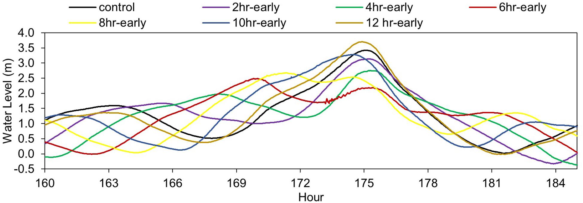
Figure 8. Simulated time series of the storm tide at The Battery based on the control run and numerical experiments. Horizontal axis is the simulation time from October 22, 1800 UTC.

According to the calculated storm tides at The Battery, one could expect that NYC would not have flooded if Hurricane Sandy had struck the region 6 h earlier. However, the model results suggest that a worst-case scenario, in terms of the extent of coastal flooding, would have occurred in lower Manhattan. If Sandy’s storm surge had arrived 6 h earlier, the extent of flooding would have been much wider than that on October 29–30, 2012 (Figure 9A). While the total flooded area (where area represents open spaces) during Hurricane Sandy, regardless of the flood depth and duration, is calculated to be 4.34 km² (control run), a 6 h shift in the storm arrival time results in a total flooded area of 7.33 km². In other words, if the storm surge had arrived 6 h earlier, the extent of flooding would have been about 69% wider.

FIGURE 9

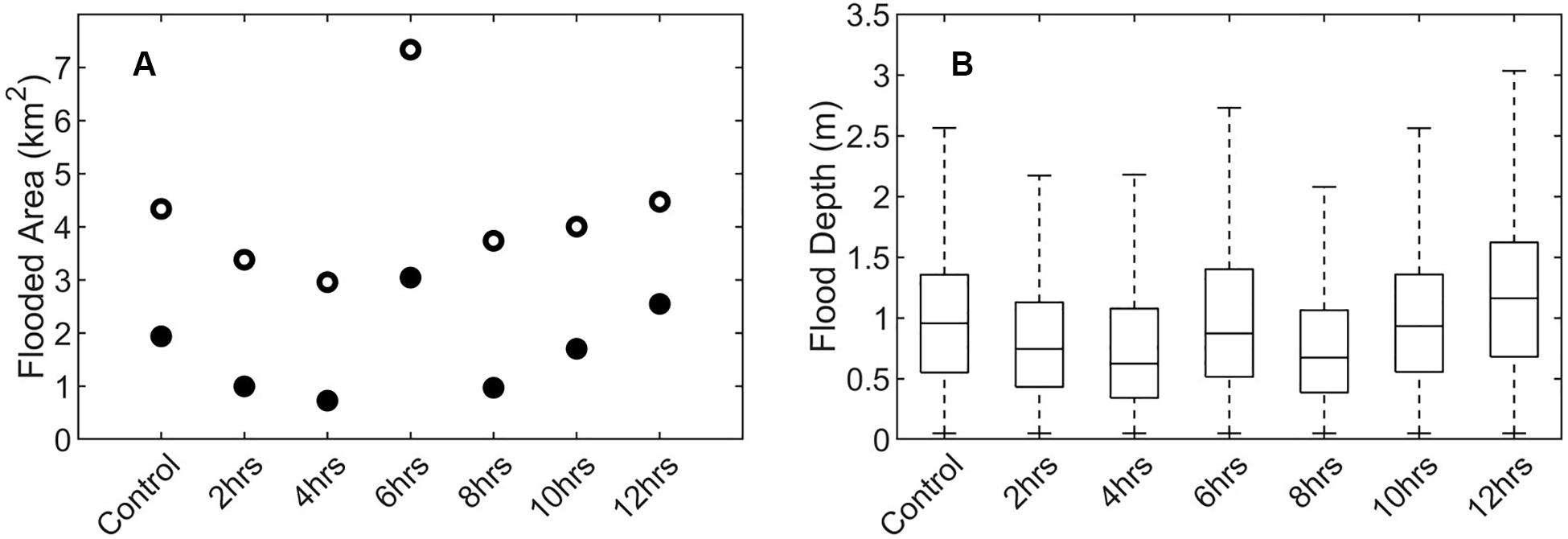
Figure 9. (A) Flooded area (solid circles represent the area with a flood depth greater than 1 m; hollow circles represent the total flooded area). Area represents the area of open spaces and excludes the area occupied by buildings. (B) Temporal maximum flood depth. The central mark on each box indicates the median (of flood depth in flooded computational nodes), the top and bottom edges of each box indicate the 25th and 75th percentiles, and the whiskers extend to the most extreme flood depths.

Model results (Figure 9B) suggest that only the 12 h early experiment shows an increase in the maximum flood depth in the study area. Although the 6 h early experiment showed a substantial increase in the extent of flooding, it shows a slight decrease in the overall maximum flood depth in the study area. The flood depth in half of the total flooded area is smaller than 0.96 m based on the control run and 0.87 m based on the 6 h early experiment. However, in many neighborhoods, especially the western part of Manhattan, the local maximum flood depth based on the 6 h early experiment is calculated to be much deeper than that based on the control run (Figure 10).

FIGURE 10

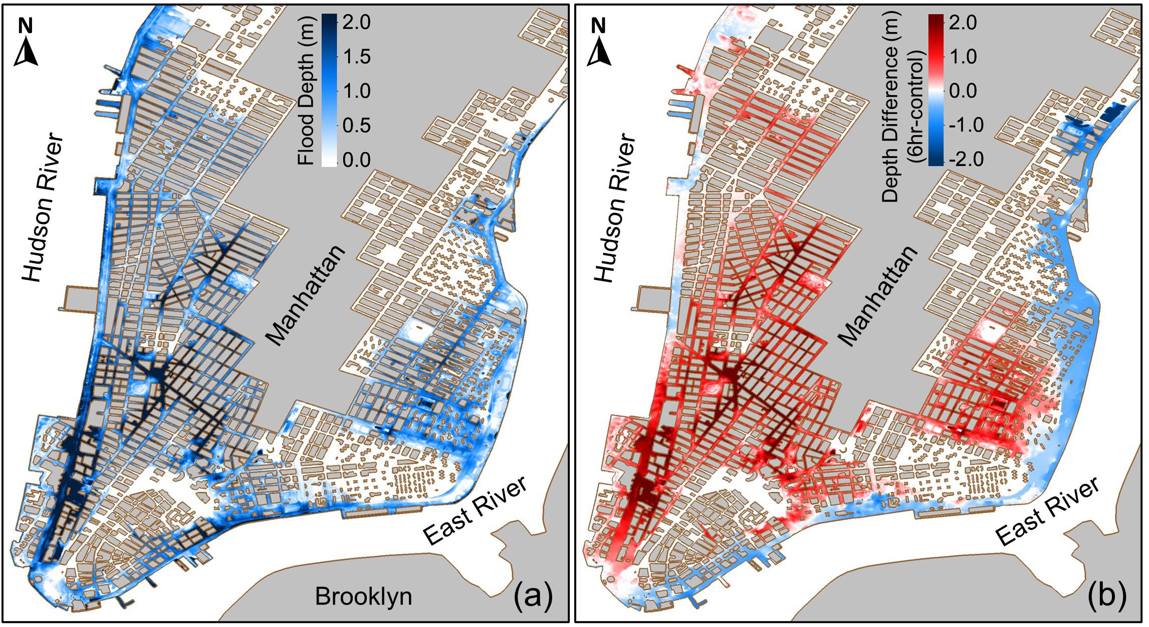
Figure 10. (a) Spatial distribution of maximum flood depth in the study area based on the 6 h early experiment and (b) the difference in the maximum flood depth based on the control run and the 6 h early experiment.

The 6 h early experiment showed the largest extent of flooding in the study area, although the simulated peak storm tide at The Battery (2.49 m) does not exceed the seawall height (2.50 m). This is because the storm tide level varies in space, depending on the bathymetry and shoreline geometry. Model results (not shown here) indicate that the peak storm tide, for short periods of time, exceeds the seawall height along the shorelines of the East River (east of Manhattan) and several locations along the Hudson River (west of Manhattan). We find that the floodwater speed based on the 6 h early experiment is much higher than that based on the control run, which explains the wider extent of flooding in the study area. A faster floodwater contains more kinetic energy, which provides the flood wave with enough momentum to overcome dissipating forces such as bottom friction and, in turn, to propagate longer distances. During coastal flood events in urban environments, narrow streets with buildings along both sides can become open channels that convey floodwaters to areas hundreds-to-thousands of meters away from the shoreline. The small bottom friction coefficient of roads and sidewalks (which are usually paved with asphalt/concrete surfaces) results in a smaller dissipation of the kinetic energy.

Figure 11 shows the time series of floodwater depth and speed at two locations on the western side of Manhattan (see Figure 3 for the location of sites). Both the peak floodwater depth and speed based on the 6 h early experiment are larger than those based on the control run. Time series based on the 6 h early experiment show substantially faster floodwaters, which explain the wider extent of flooding calculated by the 6 h early experiment compared to the control run. Figure 12 indicates that, overall, the temporal maximum floodwater speed based on the 6 h early experiment is larger than that based on the control run and other experiments. For example, while the median maximum speed based on the control run is 0.9 m.s^–1 (i.e., the maximum speed in half of the flooded computational nodes is less than 0.9 m.s^–1), the median maximum speed based on the 6 h early experiment is 1.76 m.s^–1.

FIGURE 11

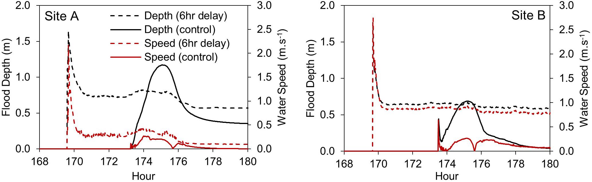
Figure 11. Time series of floodwater depth and speed at (A) site A and (B) site B located in western part of Manhattan (see Figure 3 for the site locations).

FIGURE 12

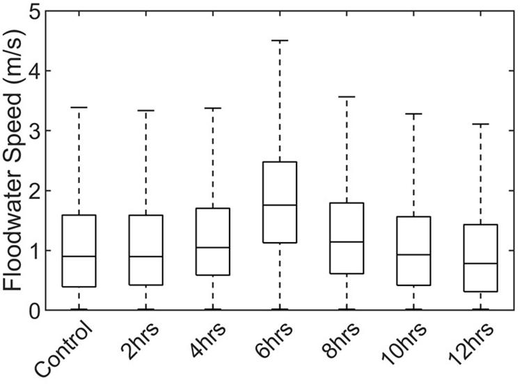
Figure 12. Temporal maximum floodwater speed. The central mark on each box indicates the median (of water speed in flooded computational nodes). The top and bottom edges of each box indicate the 25th and 75th percentiles, and the whiskers extend to the most extreme floodwater speeds.

The faster floodwater speed calculated based on the 6 h early experiment can be due to the interactions of storm surge and tides in the surrounding waters of Manhattan. Model results for the 6 h early experiment show that the storm tide in Western Long Island Sound and the East River is much larger than that based on the control run, which is consistent with findings from Georgas et al. (2014). The higher storm tides in Western Long Island Sound propagate into the East River and toward NY/NJ Harbor, in contrast to the control run that the storm tide propagates from NY/NJ Harbor to the East River (Figure 13A). In an area between the Governors Island and the southern tip of Manhattan, the water flow in the East River confronts the storm tide that propagates up NY/NJ Harbor from the Atlantic Ocean (Figure 13B). Strong flows in the East River add additional momentum to the flow in NJ/NJ Harbor which, in turn, generate energetic floodwaters on the floodplains that propagate a large area over land.

FIGURE 13

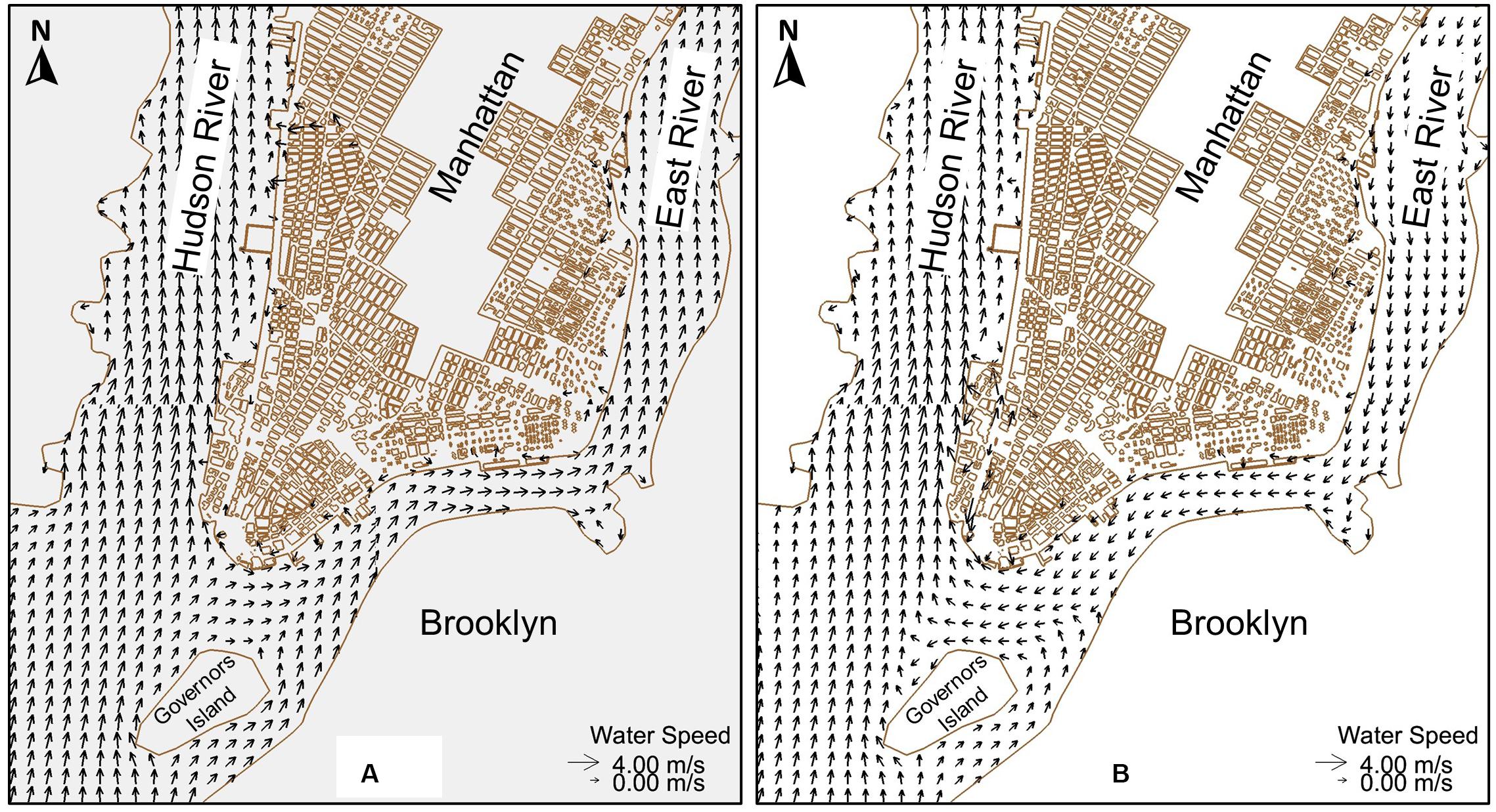
Figure 13. Water velocity fields 20 min after the flood arrival in Manhattan (A) control run and (B) 6 h early experiment.

Conclusion

Using a high-resolution hydrodynamic model, we studied the effects of tidal timing on coastal flooding induced by Hurricane Sandy in New York City. The model resolves urban features such as seawalls and buildings in Manhattan, with a spatial resolution between 3 and 8 m. Model validation against high-water-mark measurements showed a root-mean-square-error of 15 cm and a bias of 7 cm. We utilized the validated model to simulate a series of numerical experiments and to quantify the effects of tide timing on the depth and extent of flooding in low-lying areas of Manhattan.

Numerical experiments showed that if Hurricane Sandy had arrived 12 h earlier than its actual arrival time, the peak storm tide at The Battery tide gauge station, located immediately off of the shoreline in the southern tip of Manhattan, would have been 0.28 m (i.e., 8.2%) larger than the measured peak storm tide. The extent of flooding in Manhattan would have been 3% larger if Sandy had arrived 12 h earlier. On the other hand, if Hurricane Sandy had arrived 6 h earlier than it did, while the peak storm tide at The Battery would have been 0.93 m (i.e., 27%) smaller than the measured peak storm tide, the extent of coastal flooding in Manhattan would have been 69% larger.

The study showed that the storm tide level in the coastal ocean alone is not a good indicator of the extent of coastal flooding on floodplains. For example, model results showed that if Sandy’s storm surge had arrived 6 h earlier, while the peak storm tide at The Battery would have been 2.49 m, which is just below the seawall height, a large area in Manhattan would have been flooded. We found that floodwater speed substantially influences the extent of flooding. Model results showed that while the maximum floodwater speed in half of the flooded areas in Manhattan was 0.9 m.s^–1 during Hurricane Sandy, it would have been 1.76 m.s^–1 if Sandy had arrived 6 h earlier. More energetic floodwaters are caused by storm tides that propagate from the East River (Western Long Island Sound) and the Atlantic Ocean to NY/NJ Harbor in an opposing direction and consequently confront in coastal waters between Governors Island and Manhattan.

Model results presented in this study suggest that the storm tide level at a single location, e.g., The Battery for our study area, is not a good indicator of the intensity and extent of coastal flooding. Flood maps that are generated based on the storm tide at a single location may misrepresent the actual hazard in coastal floodplains, especially in the built environment. For instance, using the “bathtubbing” approach to produce flood maps based on the water level calculated by the 6 h early experiment would result in no flooding in Manhattan (as the peak storm tide level at The Battery is just below the seawall height). However, the hydrodynamic modeling approach adopted in this study showed that the 6 h early experiment produces the largest extent of flooding in Manhattan. High-resolution hydrodynamic models that resolve urban features such as buildings and streets are the most appropriate tool to reliably map coastal flood hazards in urban environments.

This study revealed the importance of tide timing on compound flooding due to tides and storm surges in Manhattan. Historical storms, e.g., Hurricane Harvey in 2017, have shown that the rainfall runoff and river flow could also have a profound effect on the extent and depth of flooding in coastal cities. Our future studies would further investigate the contribution of stormwater runoff and river discharge to compound flooding in the study area.

Data Availability Statement

The meteorological data for Hurricane Sandy were obtained from Oceanweather Inc. Tide data are available on https://www.tpxo.net/home. Measured high-water marks are available on the USGS Flood Event Viewer website (https://stn.wim.usgs.gov/FEV/). Storm tide observations are from the NOAA Tides and Currents (https://tidesandcurrents.noaa.gov/). The outputs of the numerical simulations are available upon request to the authors.

Author Contributions

RM and YW developed the computational domain and setup the model inputs. RM performed the numerical simulations and wrote the manuscript. YW edited the manuscript. All authors contributed to the article and approved the submitted version.

Conflict of Interest

The authors declare that the research was conducted in the absence of any commercial or financial relationships that could be construed as a potential conflict of interest.

Acknowledgments

We thank Dr. Andrew Cox from Oceanweather Inc. for providing us with the meteorological reanalysis data for Hurricane Sandy.

Footnotes

1. ^ www.oceanweather.com

References

An, H., and Yu, S. (2012). Well-balanced shallow water flow simulation on quadtree cut cell grids. Adv. Water Resour. 39, 60–70. doi: 10.1016/j.advwatres.2012.01.003

CrossRef Full Text | Google Scholar

Aquaveo (2013). SMS User Manual (v11.1) Surface-Water Modeling System. Provo: Aquaveo, LLC.

Google Scholar

Aronica, G., Tucciarelli, T., and Nasello, C. (1998). 2D multilevel model for flood wave propagation in flood-affected areas. J. Water Res. Plan Manag. 124, 210–217. doi: 10.1061/(asce)0733-9496(1998)124:4(210)

CrossRef Full Text | Google Scholar

Bermúdez, M., Cea, L., and Sopelana, J. (2019). Quantifying the role of individual flood drivers and their correlations in flooding of coastal river reaches. Stochast. Environ. Res. Risk Assess. 33, 1851–1861. doi: 10.1007/s00477-019-01733-1738

CrossRef Full Text | Google Scholar

Blake, E. S., Kimberlain, T. B., Berg, R. J., Cangialosi, J. P., and Beven, J. L. (2013). Tropical Cyclone Report Hurricane Sandy (Rep. AL182012). Miami, FL: National Hurricane Center.

Google Scholar

Blumberg, A., Georgas, N., Yin, L., Herrington, T., and Orton, P. (2015). Street-Scale modeling of storm surge inundation along the New Jersey Hudson River Waterfront. J. Atmos. Ocean. Technol. 32, 1486–1497. doi: 10.1175/jtech-d-14-00213.1

CrossRef Full Text | Google Scholar

Booij, N., Ris, R. C., and Holthuijsen, L. H. (1999). A third-generation wave model for coastal regions. 1: model description and validation. J. Geophys. Res. 104, 7649–7666. doi: 10.1029/98JC02622

CrossRef Full Text | Google Scholar

Bunya, S., Dietrich, J. C., Westerink, J. J., Ebersole, B. A., Smith, J. M., Atkinson, J. H., et al. (2010). A high-resolution coupled riverine flow, tide, wind, wind wave, and storm surge model for southern louisiana and mississippi. part i: model development and validation. Month. Weath. Rev. 138, 345–377. doi: 10.1175/2009mwr2906.1

CrossRef Full Text | Google Scholar

Cea, L., Garrido, M., and Puertas, J. (2010). Experimental validation of two-dimensional depth-averaged models for forecasting rainfall-runoff from precipitation data in urban areas. J. Hydrol. 382, 88–102. doi: 10.1016/j.jhydrol.2009.12.020

CrossRef Full Text | Google Scholar

City of New York (2013). Strategic Initiative for Rebuilding and Resiliency (SIRR). A Stronger, More Resilient New York. Available online at: https://www1.nyc.gov/site/sirr/report/report.page

Google Scholar

Cooperative Institute for Research in Environmental Sciences (2014). Continuously Updated Digital Elevation Model (CUDEM) - 1/9 Arc-Second Resolution Bathymetric-Topographic Tiles. [Indicate Subset Used]. Silver Spring, MD: NOAA National Centers for Environmental Information.

Google Scholar

Department of Information Technology and Telecommunications (2013). Available online at: https://data.cityofnewyork.us/City-Government/1-foot-Digital-Elevation-Model-DEM-/dpc8-z3jc (accessed August 2019).

Google Scholar

Department of Information Technology and Telecommunications (2016). Available online at: https://github.com/CityOfNewYork/nyc-geo-metadata/blob/master/Metadata/Metadata_BuildingFootprints.md (accessed April 2019).

Google Scholar

Dietrich, J. C., Zijlema, M., Westerink, J. J., Holthuijsen, L. H., Dawson, C., Luettich, R. A., et al. (2011). Modeling hurricane waves and storm surge using integrally-coupled, scalable computations. Coast. Eng. 58, 45–65. doi: 10.1016/j.coastaleng.2010.08.001

CrossRef Full Text | Google Scholar

Egbert, G. D., and Erofeeva, S. Y. (2002). Efficient inverse modeling of barotropic ocean tides. J. Atmos. Ocean. Technol. 19, 183–204. doi: 10.1175/1520-0426(2002)019<0183:eimobo>2.0.co;2

CrossRef Full Text | Google Scholar

Gallien, T. W., Schubert, J. E., and Sanders, B. F. (2011). Predicting tidal flooding of urbanized embayments: a modeling framework and data requirements. Coast. Eng. 58, 567–577. doi: 10.1016/j.coastaleng.2011.01.011

CrossRef Full Text | Google Scholar

Georgas, N., Orton, P., Blumberg, A., Cohen, L., Zarrilli, D., and Yin, L. (2014). The impact of tidal phase on hurricane Sandy’s flooding around New York City and Long Island sound. J. Extreme Events 1:67.

Google Scholar

Lin, N., Kopp, R. E., Horton, B. P., and Donnelly, J. P. (2016). Hurricane Sandy’s flood frequency increasing from year (1800) to 2100. Proc. Natl. Acad. Sci. U.S.A. 113, 12071–12075. doi: 10.1073/pnas.1604386113

PubMed Abstract | CrossRef Full Text | Google Scholar

Luettich, R. A. Jr., Westerink, J. J., and Scheffner, N. W. (1992). ADCIRC: An Advanced Three-Dimensional Circulation Model for Shelves, Coasts and Estuaries. Report 1. Theory and methodology ofADCIRC-2DDI and ADCIRC-3DL (Tech. Rep. DRP-92-6). Vicksburg, MS: U.S. Army Corps of Engineers.

Google Scholar

Lyddon, C. E., Brown, J. M., Leonardi, N., Saulter, A., and Plater, A. J. (2018). Quantification of the uncertainty in Coastal storm hazard predictions due to wave-current interaction and wind forcing. Geophys. Res. Lett. 46, 14576–14585. doi: 10.1029/2019GL086123

CrossRef Full Text | Google Scholar

Marsooli, R., and Lin, N. (2018). Numerical modeling of historical storm tides and waves and their interactions along the U.S. East and Gulf Coasts. J. Geophys. Res. Oceans 123, 3844–3874. doi: 10.1029/2017JC013434

CrossRef Full Text | Google Scholar

Marsooli, R., Orton, P., Mellor, G., Georgas, N., and Blumberg, A. (2017). A coupled circulation-wave model for numerical simulation of storm tides and waves. J. Atmos. Ocean. Technol. 34, 1449–1467. doi: 10.1175/jtech-d-17-0005.1

CrossRef Full Text | Google Scholar

Nicholls, R. J., Hanson, S., Herweijer, C., Patmore, N., Hallegatte, S., Corfee-Morlot, J., et al. (2007). Ranking Port Cities With High Exposure and Vulnerability to Climate Extremes—Exposure Estimates. OECD environmental working paper no. 1. Paris: Organization for Economic Co-operation and Development (OECD).

Google Scholar

Orton, P., Hall, T. M., Talke, S. A., Blumberg, A. F., Georgas, N., and Vinogradov, P. S. M. (2016). A validated tropical-extratropical flood hazard assessment for New York harbor. J. Geophys. Res. Oceans 121, 8904–8929.

Google Scholar

Orton, P. N., Lin, V., Gornitz, B., Colle, J., Booth, K., and Feng, et al. (2019). New York City panel on climate change 2019 report chapter 4: coastal flooding. Ann. N. Y. Acad. Sci. 1439, 95–114. doi: 10.1111/nyas.14011

PubMed Abstract | CrossRef Full Text | Google Scholar

Ris, R. C., Holthuijsen, L. H., and Booij, N. (1999). A third-generation wave model for coastal regions: 2. verification. J. Geophys. Res. 104, 7649–7666. doi: 10.1029/1998JC900123

CrossRef Full Text | Google Scholar

Roberts, K. J., and Pringle, W. J. (2018). OceanMesh2D: User Guide – Precise Distance-Based Two-Dimensional Automated Mesh Generation Toolbox Intended for Coastal Ocean/Shallow Water. Computational Hydraulics Lab. University of Notre Dame, United States. doi: 10.13140/RG.2.2.21840.61446/2

PubMed Abstract | CrossRef Full Text | Google Scholar

Roberts, K. J., Pringle, W. J., and Westerink, J. J. (2019). OceanMesh2D 1.0: MATLAB-based software for two-dimensional unstructured mesh generation in coastal ocean modeling. Geosci. Model Dev. 12, 1847–1868. doi: 10.5194/gmd-12-1847-2019

CrossRef Full Text | Google Scholar

Schubert, C. E., Busciolano, R., Hearn, P. P. Jr., Rahav, A. N., Riley, B., Jason, F., et al. (2015). Analysis of Storm-Tide Impacts from Hurricane Sandy in New York. U.S. Geological Survey Scientific Investigations Report 2015-5036. Anchorage, AK: UGSC.

Google Scholar

Schubert, J. E., and Sanders, B. F. (2012). Building treatments for urban flood inundation models and implications for predictive skill and modeling efficiency. Adv. Water Resour. 41, 49–64. doi: 10.1016/j.advwatres.2012.02.012

CrossRef Full Text | Google Scholar

Schubert, J. E., Sanders, B. F., Smith, M. J., and Wright, N. G. (2008). Unstructured mesh generation and landcover-based resistance for hydrodynamic modeling of urban flooding. Adv. Water Resour. 31, 1603–1621. doi: 10.1016/j.advwatres.2008.07.012

CrossRef Full Text | Google Scholar

Sopelana, J., Cea, L., and Ruano, S. (2018). A continuous simulation approach for the estimation of extreme flood inundation in coastal river reaches affected by meso and macro tides. Nat. Hazards 93, 1337–1358. doi: 10.1007/s11069-018-3360-3366

CrossRef Full Text | Google Scholar

Takagi, H., Li, S., Leon, M. D., Esteban, M., Mikami, T., Matsumaru, R., et al. (2016). Storm surge and evacuation in urban areas during the peak of a storm. Coast. Eng. 108, 1–9. doi: 10.1016/j.coastaleng.2015.11.002

CrossRef Full Text | Google Scholar

Tozer, B., Sandwell, D. T., Smith, W. H. F., Olson, C., Beale, J. R., and Wessel, P. (2019). GlobalBathymetryandTopographyat15ArcSec: SRTM15+. Earth Space Sci. 6, 1847–1864. doi: 10.1029/2019ea000658

CrossRef Full Text | Google Scholar

Valle-Levinson, A., Olabarrieta, M., and Heilman, L. (2020). Compound flooding in houston-galveston Bay during Hurricane Harvey. Sci. Total Environ. 747:141272. doi: 10.1016/j.scitotenv.2020.141272

PubMed Abstract | CrossRef Full Text | Google Scholar

Wang, H. V., Loftis, J. D., Liu, Z., Forrest, D., and Zhang, J. (2014). The storm surge and sub-grid inundation modeling in New York City during Hurricane Sandy. J. Mar. Sci. Eng. 2, 226–246. doi: 10.3390/jmse2010226

CrossRef Full Text | Google Scholar

Westerink, J. J., Luettich, R. A. Jr., Blain, C. A., and Scheffner, N. W. (1994). ADCIRC: An Advanced Three-Dimensional Circulation Model for Shelves, Coasts and Estuaries. Report 2: users’ manual for ADCIRC-2DDI (Tech. Rep. DRP-92-6). Vicksburg, MS: U.S. Army Corps of Engineers.

Google Scholar

Westerink, J. J., Luettich, R. A., Feyen, J. C., Atkinson, J. H., Dawson, C., Roberts, H. J., et al. (2008). A basin- to channel-scale unstructured grid hurricane storm surge model applied to Southern Louisiana. Month. Weath. Rev. 136, 833–864. doi: 10.1175/2007MWR1946.1

CrossRef Full Text | Google Scholar

Yin, J., Lin, N., and Yu, D. (2016). Coupled modeling of storm surge and coastal inundation: a case study in New York City during Hurricane Sandy. Water Resour. Res. 52, 8685–8699. doi: 10.1002/2016WR019102

CrossRef Full Text | Google Scholar

Zhong, H., Van Overloop, P. J., and Van Gelder, P. H. A. J. M. (2013). A joint probability approach using a 1D hydrodynamic model for estimating high water level frequencies in the Lower Rhine Delta. Nat. Hazards Earth Syst. Sci. 13, 1841–1852. doi: 10.5194/nhess-13-1841-2013

CrossRef Full Text | Google Scholar