Empirically Modeling the Energy Implications of Cool Roof Retrofits

Introduction

Almost 90% of United States homes now use space cooling (Doe (U.S. Department of Energy), 2017b). Thus, cost-effective strategies to reduce energy consumed for cooling are critical to improving the performance of the U.S. energy system.

In warm climates, a significant passive heat load may enter the building through the roof (Nahar et al., 2003). Passive design strategies can mitigate excess heat loads using either natural ventilation, thermal insulation, orientation, evaporation, or solar reflectance (Hernández-Pérez et al., 2014). All else equal, white roofs will reflect more sunlight than dark roofs, reducing a building’s heat gain.

In addition to albedo, a roof’s thermal emittance, or its propensity to emit thermal radiation, can also impact thermal performance. Highly emissive roofing materials, such as most asphalt shingles, will radiate more stored heat away from the building than lower emissivity materials, such as bare metal roofs. However, most research indicates that roof albedo dominates a roof’s effect on building cooling (Akbari and Konopacki, 1998; de Brito Filho et al., 2011; Al-Obaidi et al., 2014; Brito Filho and Santos, 2014). In cooler climates, however, less emissive materials can beneficially store and indirectly transfer heat into buildings during the heating season.

The thermal effects of building albedo change are relatively well understood. Hernández-Pérez et al. (2014) review several decades of building albedo research, identifying 42 studies applying theoretical models of building albedo, 18 field trials, 10 studies of albedo change on existing buildings, and 8 studies using calibrated theoretical models. Collectively, these studies produce a high pedigree of confidence that higher albedo building surfaces reduce building cooling site energy use, with the magnitude of any given reduction being influenced by the degree of albedo change, building-level characteristics, and climate.

Studies also indicate that site heating energy use increases with increasing albedo, typically referred to as the “heating penalty.” However, studies find few contexts in which the heating penalty outweighs the environmental or monetary benefits of cool roofs (Akbari and Konopacki, 1998; Hosseini and Akbari, 2014). For example, Synnefa et al. (2007) use theoretical building energy demand models to explore global variation in site cooling energy use in homes retrofitted with a cool roof coating. For a solar reflectance change to 0.85 from 0.20, they estimate reductions in end use consumption for cooling exceeding any increases in heating site energy use for 26 of 27 global cities, with the heating penalty in Mexico City being slightly larger than the reduction in site cooling energy use. If losses in electric power generation and transmission were included, the results would likely show primary energy savings for all locations.

Growing awareness of cool roof performance has prompted research estimating outcomes from widespread cool roof adoption and respective implications for policy. Levinson and Akbari (2010) estimate that retrofitting 80% of U.S. commercial buildings with a white roof would reduce cooling site energy use by 37 PJ per year and provide HVAC energy cost savings of $735 million per year. State estimates of site cooling energy reductions vary from 12 to 28 MJ per year per m² of roof (mean of 18), and site heating energy penalties range from 0.32 to 15 MJ per year per m² of roof (mean of 6.9). Coupling their results with state energy prices and regional power grid emissions, Levinson and Akbari (2010) estimate net monetary savings and reductions in CO₂, NO_X, SO₂, and Hg for all U.S. states, even when including a heating penalty.

Sproul et al. (2014) perform a similar techno-economic assessment of traditional black, white, and green roof alternatives using literature estimates and data from 22 roof projects in diverse U.S. cities. Including installation and maintenance costs, electricity grid emissions, equipment downsizing for stormwater and cooling, and avoided storm water fees, they estimate that white roofs outperform black roofs for all 22 projects and outperform green roofs in 21 projects, with a representative white roofs lifetime savings of $96 per m² and $26 per m² relative to green and black roofs, respectively.

By reducing the thermal extremes to which roofs are exposed, white roof coatings may also increase the useful roof service life over and above darker materials, and such benefits are often cited by policy makers (Doe (U.S. Department of Energy), 2017a). Industry estimates suggest that coatings can increase the service life of conventional commercial roofs by 5–15 years for a diverse type of roof materials (APOC, 2017). However, I identified no empirical information describing the observed increase in roof service life from coatings.

Policy makers have responded to the opportunities of cool roofs by encouraging adoption using a mix of financial incentives, standards, and labeling schemes. The Cool Roof Rating Council (2017) indicates that 17 municipalities (across 13 states), 7 states, and the U.S. Internal Revenue Service offer rebates for cool roofs. The U.S. Energy Star program promulgated its first consumer label for cool roof products in 1999, which has since been revised twice (Energy Star, 2017). Researchers have previously recommended changes to California’s building energy code on the basis of theoretical energy reductions from cool roofs (Levinson et al., 2005; Rosado and Levinson, 2019).

Measuring the performance of cool roofs adopted in response to current policies requires methods different from those theoretical techniques profiled above. Theoretical models and field trials can treat influential parameters (e.g., envelope insulation) parametrically when estimating performance. However, such influential variables are unobserved in the context of current policies aiming to influence consumer choices. Policy makers simply offer an incentive or provide a label but do not get to prescribe the occupancy or building characteristics associated with affected retrofits. As a result, methods that accommodate unobserved participant heterogeneity or selection bias are needed to estimate roof performance in the context of current adoption policies. For example, occupant behavior, which is not integrated into current theoretical models, has been shown to significantly affect roof performance (Pisello et al., 2015).

The difference-in-differences (DiD) method is a quasi-experimental technique that utilizes longitudinal data to “difference out” group effects that could otherwise influence measured outcomes. Equation 1 presents the basic DiD model.

$$Y_{i,t}={\mathrm{\beta }}_0+{\mathrm{\beta }}_{1}trea{t}_i+{\mathrm{\beta }}_{2}pos{t}_t+D\left(trea{t}_i\times pos{t}_t\right)+{\mathrm{\epsilon }}_{i,t}(1)$$

where Y_i,t = outcome for unit i at time t

treat_i = group indicator distinguishing for treated units (0 = control; 1 = treated)

post_t = indicator for the treatment period (0 = prior to treatment; 1 = post treatment)

β₀,β₁,β₂ = estimated model coefficients

D = difference-in-differences estimate or the effect of the treatment

ε_i,t = error term.

Consider comparing expected values (E[Y]) for two groups (a treated and a control) with one common treatment period (treat = 0 before treatment and treat = 1 after treatment).

E[Y_{treat = 1,post = 0}] = β₀ + β₁ = before treatment, treated group

E[Y_{treat = 1,post = 1}] = β₀ + β₁ + β₂ + D = after treatment, treated group

E[Y_{treat = 1,post = 0}]−E[Y_{treat = 1,post = 1}] = β₂ + D = average effect of treatment on treated group.

By modeling differences in the outcome, Y, within a treated group over time, the group-level term, β₁, has been “differenced out.” Controlling for group effects is important if the treatment group demonstrates tendencies that influence Y that are otherwise unrelated to the treatment. For example, homeowners choosing a white roof might also have higher site cooling energy use as a result of poor insulation. Without a group effect that controls for this, the effect of attic insulation could be improperly attributed to whitening. This first difference, D + β₂, represents the average effect of the treatment comparing the treated group before and after treatment, which includes both the outcome of interest, D, and a time effect, β₂. The parameter β₂ represents any impacts to energy use that occurred in the treatment period unrelated to the treatment itself. By modeling a second “difference” across control and treatment groups, one can find this time effect as follows.

E[Y_{treat = 0,post = 0}] = β₀ = outcome before treatment, control group

[Y_{treat = 0,post = 1}] = β₀ + β₂ = outcome after treatment, control group

E[Y_{treat = 0,post = 0}]−E[Y_{treat = 0,post = 1}] = β₂ = fixed effect for treatment period.

The second difference, E[Y_{treat = 0,post = 0}]−E[Y_{treat = 0,post = 1}] or β₂ is the average difference for the control group before and after the treatment period. This difference should represent any time effects unrelated to the treatment. A final “difference-in-differences” produces the estimate of interest, D.

$${\mathrm{\beta }}_2+D-{\mathrm{\beta }}_2=D=\underset{\begin{array}{c}\hfill Averagedifferenceintreatedgroup\hfill \\ \hfill beforeandaftertreatment\hfill \end{array}}{\underbrace{E\left[Y_{treat=1,post=0}\right]-E\left[Y_{treat=1,post=1}\right]}}-\underset{\begin{array}{c}\hfill Averagedifferenceforcontrolgroup\hfill \\ \hfill beforeandaftertreatmentperiod\hfill \end{array}}{\underbrace{E[Y_{treat=0,post=0}]-E[Y_{treat=0,post=1}]}}$$

This second difference removes any confounding time effects, β₂, assuming such affects are similar for the treated and control units. This assumption is known as the “parallel trend” assumption for DiD models. DiD methods have been applied to other energy efficiency retrofits (Adan and Fuerst, 2016; Datta and Filippini, 2016; Adland et al., 2018).

Similar to existing cool roof monetary incentives encouraging adoption, residents in Austin, TX were invited to participate in an experiment in which their roofs would be coated white at no charge. Space cooling branch circuits were separately monitored on an hourly basis for both the treated homes (those choosing to whiten their roof) and a control sample. Varied empirical methods, including individual within-household comparisons and regression, were used to estimate whitening’s impact.

A life-cycle costs analysis was also conducted to gauge the secondary benefit of delaying roof replacement as a result of the added protection afforded the roof membrane by the coating materials. In addition to the benefit from delaying replacement, the life-cycle cost analysis included the costs of roof whitening (materials and labor), a heating penalty, and site cooling energy reductions estimated from the DiD model. The methods profiled herein can be generally applied to measure the performance of roof retrofits where unobserved effects influence selection or energy consumption.

Materials and Methods

Sample Preparation

Approximately 120 households across 25 ZIP codes in Austin, TX, United States were invited to participate in an experiment in which their roofs would be coated white at no charge and the effect on space cooling would be estimated. A total of seven homes were recruited.

Roofs on the treated homes (also referred to as the “coated” or “whitened” homes) were all conventional asphalt shingles that were either light gray, dark gray, or brown in color. Six of the treated homes were one story and one was three stories. The distribution of roofs slopes (rise to run) for the treated homes is 4 over 12 (n = 4), 3.5 over 12 (n = 1), 2.5 over 12 (n = 1), and a mixed slope (n = 1).

Two homes were coated in fall 2015, and the remaining five were coated in the summer and fall of 2016. Photographs of the coating used, Behr’s Multi-Surface Roof Paint (color White Reflective No. 65), are included in the Supplementary Information. Each home received two coats, the second within a week of the initial coat. The roof coating schedule is provided in the Supplementary Information. In preparing the sample for analyses, homes were indicated as coated on the date of the initial coat. Recruitment, project scheduling, and white roof coating (BEHR, 2020) were managed by the White Roof Research Project. Photographs of two coated homes are included in the Supplementary Information.

The Pecan Street Research Institute (2017) provided household characteristics data (floor space and number of floors) and metered hourly site cooling electricity use from May 2015 and October 2017. All data management, visualizations, and modeling were completed using the R language and compatible packages (Wickham, 2016; R Core Team, 2020; Wickham et al., 2020).

In an effort to reduce inflated zeros and remove observations of electricity used by heat pumps for heating, heating days were estimated and removed by comparing thermostat set points to historical temperature records. Inflated zeros can cause the distribution of observations to deviate from normality, making it harder to fit data to related statistical models. Pecan Street publishes thermostat set point data for a broader sample of homes (n = 341) than those for which cooling is monitored. The median heating (21.1°C or 70°F) and cooling (25.6°C or 78°F) thermostat set points were used as the basis for defining heating and cooling days. Only days where the mean outdoor temperature is above the median thermostat set point for heating were included in the analysis. These criteria identified 126, 128, and 123 cooling days in years 2015, 2016, and 2017, respectively, between May 2015 and October 2017. The distribution of the resulting air conditioning data still has a small amount of inflated point mass (0.3% of observations) at zero.

It was assumed that household occupants traveled during periods when at least two consecutive days during the cooling season recorded no site cooling energy use, and these periods were dropped from the analysis.

The final sample, summarized in Table 1, consists of unbalanced observations of site cooling energy use for 114 homes (7 treated and 107 controls) by date, daytime, and nighttime, where daytime and nighttime periods were distinguished by local sunrise and sunset data (U.S. Navy, 2017). The Pecan Street data identifiers used in this analysis are included in the Supplementary Information for those interested in further studying this sample.

TABLE 1

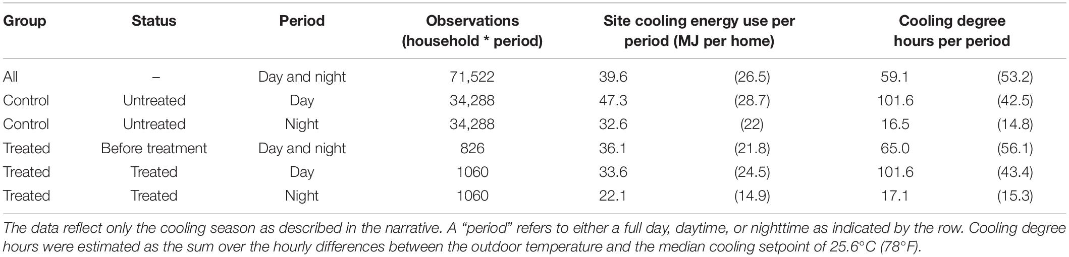
Table 1. Household-level summary statistics (mean and standard deviation) of site cooling energy use and cooling degree hours per period for 114 homes in Austin, TX, United States monitored between May 2015 and June 2017.

Figure 1 shows distributions of site cooling energy use by treatment status, experimental group, and period (day or night). Visually, whitening appears to reduce site cooling energy use, which is most apparent during daytime. During the day, the distributions for each experimental group are nearly identical when untreated, whereas consumption for the treated group appears to decrease after whitening.

FIGURE 1

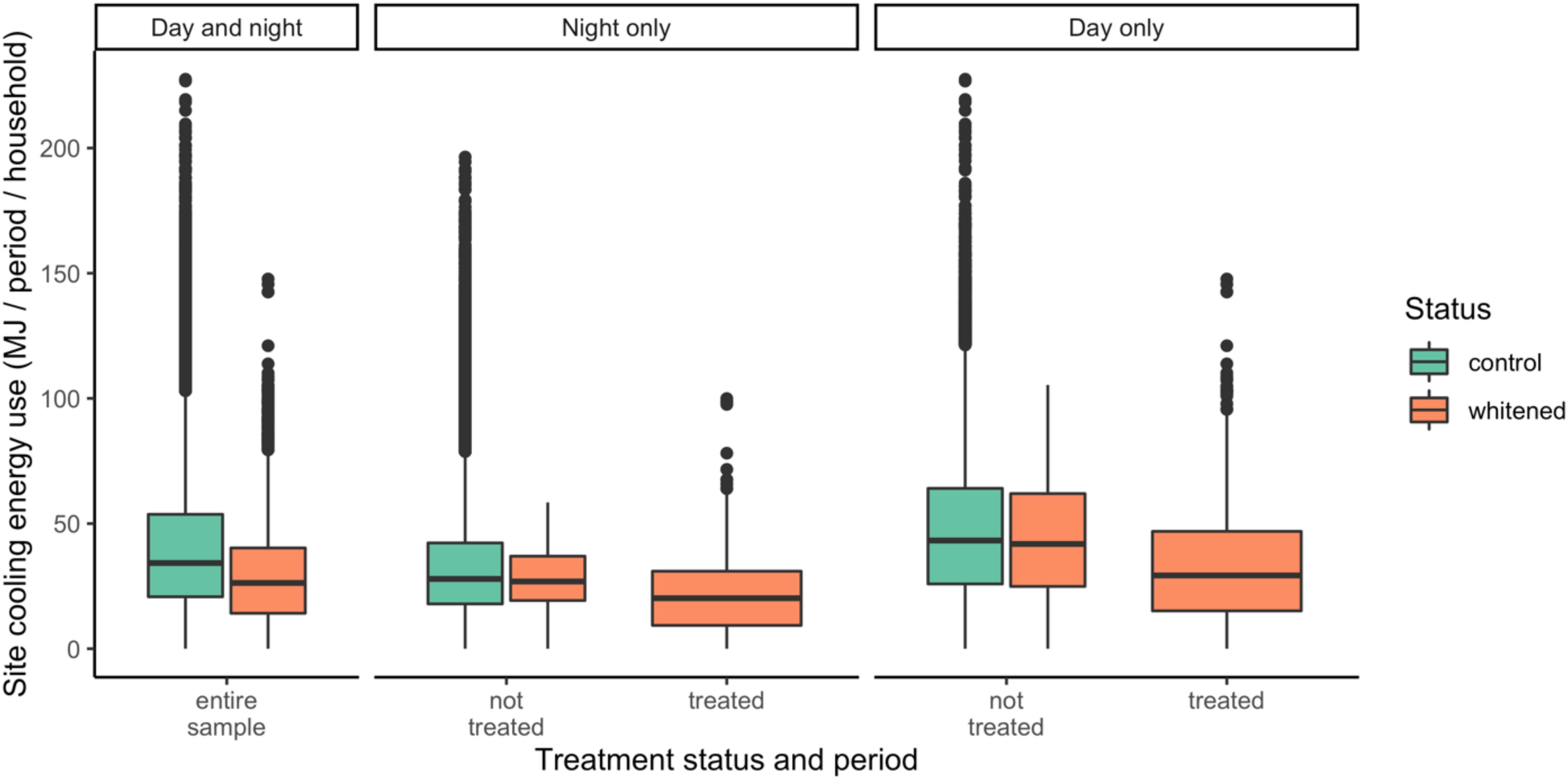
Figure 1. Household-level site cooling energy use of 114 homes in Austin, TX, United States by group (control, whitened) and period (day, night) monitored between May 2015 and June 2017.

Within-Household Comparisons

Site cooling energy use was compared before and after treatment for individual households using descriptive statistics and t-tests. Separate comparisons were made for day and night on the basis of sunrise and sunset.

Model of Site Cooling Energy Use

Individual household comparisons may be misleading for two reasons. First, factors other than whitening—both technical and behavioral—can impact whitening’s performance. If these factors correlate with whitening, their effect on site cooling energy use could be improperly associated with whitening. Second, these same factors may influence whitening’s impact. An example of this is demonstrated by showing graphically the impact of observed attic insulation on whitening’s impact in the “Results” section.

Statistical approaches are needed to estimate whitening’s impact while controlling for other influences on site cooling energy use. Equation 2 presents a two-way fixed effects model of site cooling energy use.

$$a{c}_{i,t}={\mathrm{\beta }}_0+{\mathrm{\beta }}_{post}\times pos{t}_{i,t}+{\mathrm{\beta }}_w\times w+{\mathrm{\beta }}_h\times h+{\mathrm{\epsilon }}_{i,t}(2)$$

where ac_i,t = site cooling energy use in units of MJ per period for household i at time t

post_i,t = household i whitened at time t (0 = not whitened; 1 = whitened)

w = day fixed effect

h = household fixed effect.

Equation 2 is a more generalized version of the two-period DiD model presented in Eq. 1. Equation 1 includes only one, uniform treatment period and controls for household-level variation by group. In contrast, Eq. 2 controls for individual-level household and temporal variation with fixed effects or “dummy variables,” h and w. Equation 2 is more robust than Eq. 1 and also reduces potential confounding temporal effects characteristic of DiD methods (the parallel trend assumption).

Ordinary least squares (OLS) solutions to DiD models are often prone to serial correlation (Bertrand et al., 2004). Serial correlation would imply errors are correlated by household over time. Serial correlation biases the standard errors (and thus p values) for estimated coefficients. Standard errors are clustered by household to reduce serial correlation.

In an effort to better represent the observed frequency of zero site cooling energy use, Tweedie regression was applied in addition to OLS estimators. The Tweedie distribution better accommodates the slight observed probability mass spike at zero.

The performance of reflective roofs changes at night. Differences in roof temperatures between light and dark roofs have also been observed to sustain past sunset (Parker and Barkaszi, 1997). As such, separate daytime and nighttime models have been prepared, where periods are differentiated by sunset and sunrise (U.S. Navy, 2017).

The coefficient β_post in Eq. 2 represents the average effect of whitening for the treated homes compared to two control groups: those untreated throughout the experiment and those not yet treated (Goodman-Bacon, 2018). The average effect is often of most interest to policy makers, where policies aimed at encouraging retrofits do not get to control for influential household-level variation and behavioral change may influence outcomes.

Description of Life-Cycle Cost Analysis

The subset of homes (n = 89) for which floor space and the number of floors are published (Pecan Street Research Institute, 2017) were used. The roof area for these homes was estimated as the floor space divided by the number of floors. The cost estimate sample consists of 89 homes with distributions of roof areas and air conditional site cooling energy use as described in Table 2.

TABLE 2

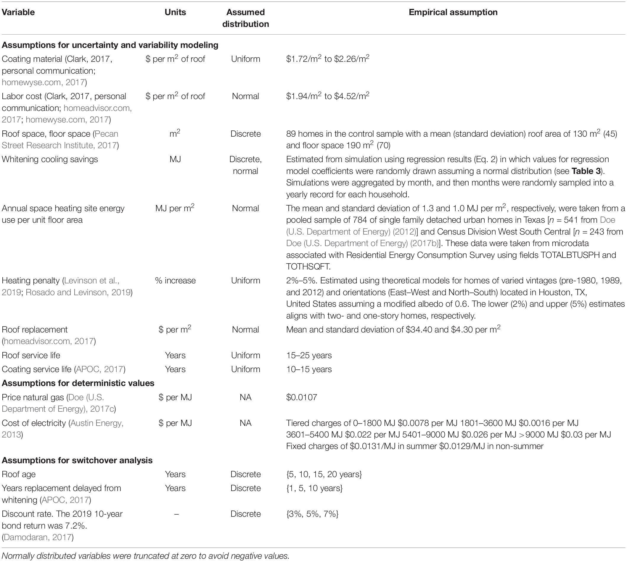
Table 2. Assumptions used for the cost analysis.

Site cooling energy use reductions were estimated by applying Eq. 2 to these 89 homes. The regression results for β_post include the only mean effect of whitening, whereas whitening’s effect is expected to vary by household. It is assumed that the distribution of β_post estimated by regression is a reasonable proxy for household-level variation in whitening’s effect. To simulate this household-level variation, 100 random samples were drawn from the distribution of β_post for each household, producing 100 different records of daily energy reductions for each household. Importantly, the assumed β_post does not change within a simulated household record, as opposed to allowing β_post to vary across days. In other words, for any given simulation, the β_post assumed for a given household is constant. Daily simulations were then aggregated by household and month, and then a representative year for each household was constructed by randomly sampling months in the observation period to moderate across the different weather patterns experienced during the experiment. The net effect of sampling produced a synthetic record of monthly cooling consumption of 4450 household^∗months.

In estimating the monetary savings from site cooling energy reductions, total electricity demand (Pecan Street Research Institute, 2017) was used in order to account for Austin’s tiered pricing schedule (Austin Energy, 2013). The remaining cost assumptions and references—including those used to estimate roof whitening costs, heating penalties, and delayed replacement benefits—are summarized in Table 2. Perhaps the most difficult of these assumptions is the expected heating penalty, modeled as a percent reduction. Previous works estimate ranges in heating penalties around 2% to 14% (Rosado and Levinson, 2019) and 10% to 30% (New et al., 2016). The latter estimated a cool roof heating penalty intensity of 1.8 MJ per m² of roof area. Applying this intensity to the 99 homes for which roof area is available would correspond to a 10% (first quartile) to 30% (third quartile) increase in site heating energy use, assuming baseline heating intensities are consistent with U.S. Department of Energy surveys (Doe (U.S. Department of Energy), 2012).

As summarized in Eq. 3 and Table 3, the life-cycle cost analysis includes a benefit for delaying roof replacement, electricity savings, the initial cost of whitening, and an annual heating penalty. Life-cycle costs are presented on a net present value basis using standard discounting. Social benefits, such as reduction in greenhouse gases, are not included in this analysis.

TABLE 3

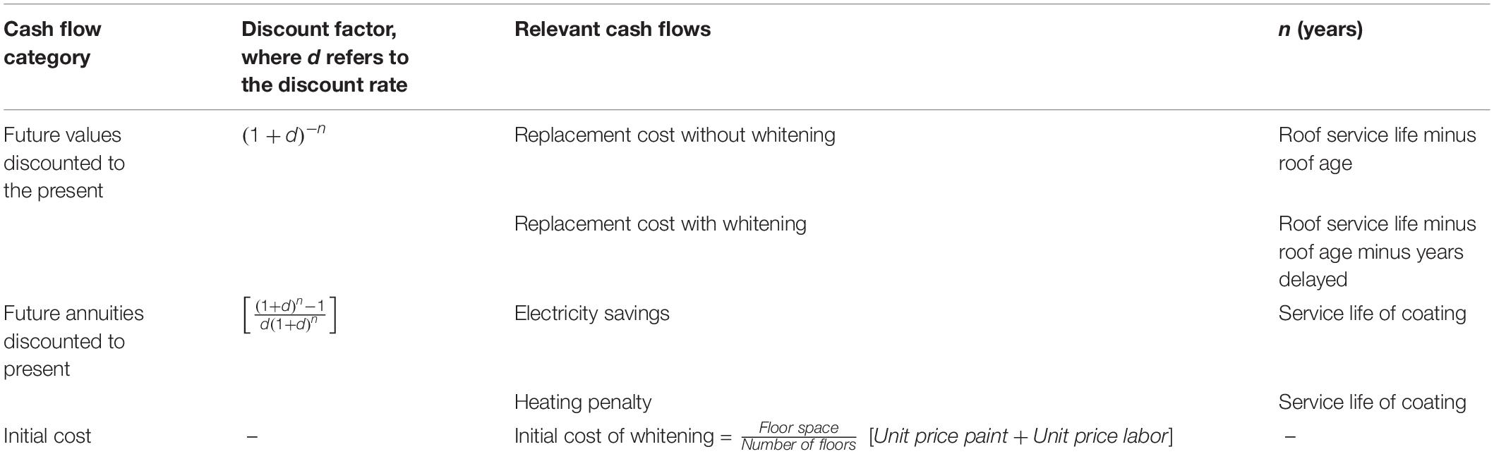
Table 3. Summary of the cash flow discounting used in the life-cycle cost analysis.

$$NPV=\underset{Benefitofdeleyedreplacement}{\underbrace{\begin{array}{c}\hfill Replacementcost\hfill \\ \hfill withoutwhitening\hfill \end{array}-\begin{array}{c}\hfill Replacementcost\hfill \\ \hfill withwhitening\hfill \end{array}}}$$

$$\mathrm{\hspace{1em}}+\begin{array}{c}\hfill Electricity\hfill \\ \hfill Savings\hfill \end{array}-\begin{array}{c}\hfill InitialCost\hfill \\ \hfill ofWhitening\hfill \end{array}-\begin{array}{c}\hfill Heating\hfill \\ \hfill Penalty\hfill \end{array}$$

Results

Table 4 summarizes the household-level comparisons before and after treatment. Table 4 indicates significant reductions at the 1% confidence level for all within-household comparisons except for daytime consumption for household 9654 and nighttime consumption for household 2158. Statistically significant percent reductions range from 14% to 49.2% during the day, and a 9.7% increase to a 40.3% decrease during nighttime.

TABLE 4

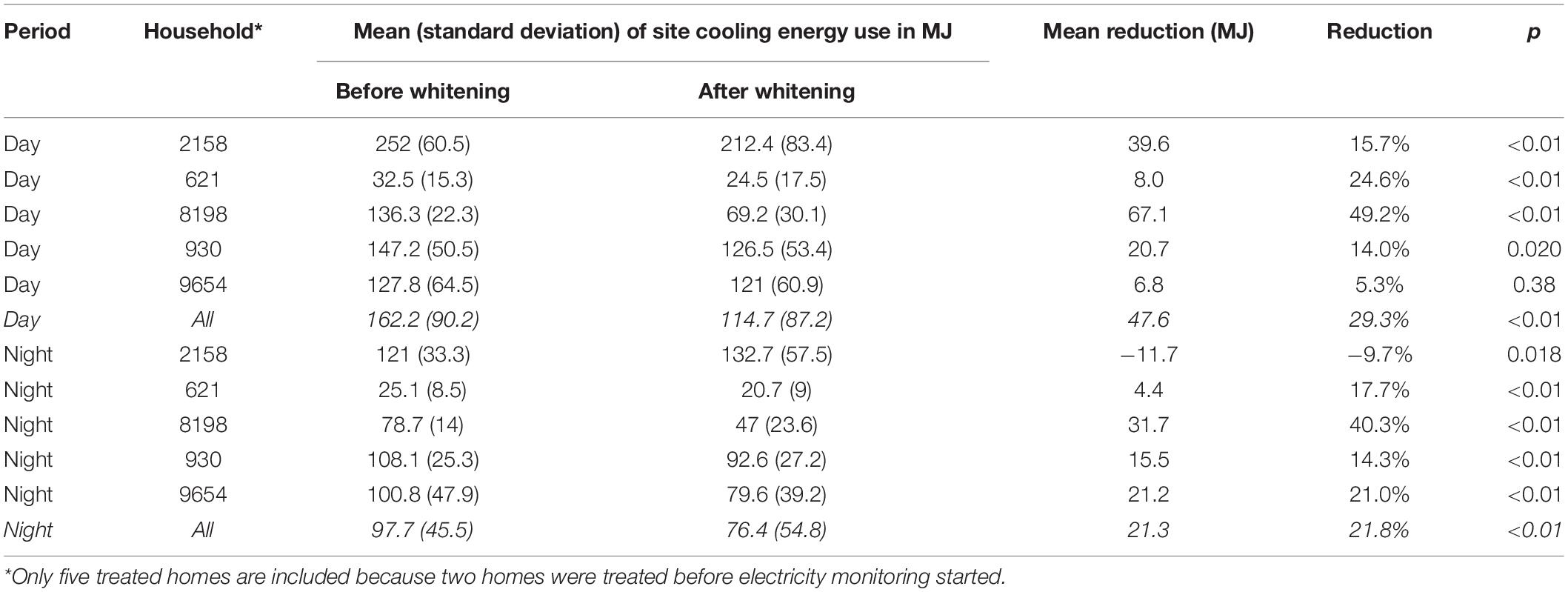
Table 4. Household-level comparisons for the treated sample.

Unobserved variation in multiple technical and behavioral factors is expected to drive the observed differences in whitening performance across households. As a demonstration, Figure 2 shows variation in site cooling energy use by the amount of attic insulation before and after whitening. Theory suggests that whitening would have a lower impact with increasing attic insulation, which is demonstrated by the two linear trends approaching each other in Figure 2. At high R values in Figure 3, the 95% confidence intervals in the trend lines nearly approach each other, suggesting that whitening may not have detectable effects for R values beyond 35.

FIGURE 2

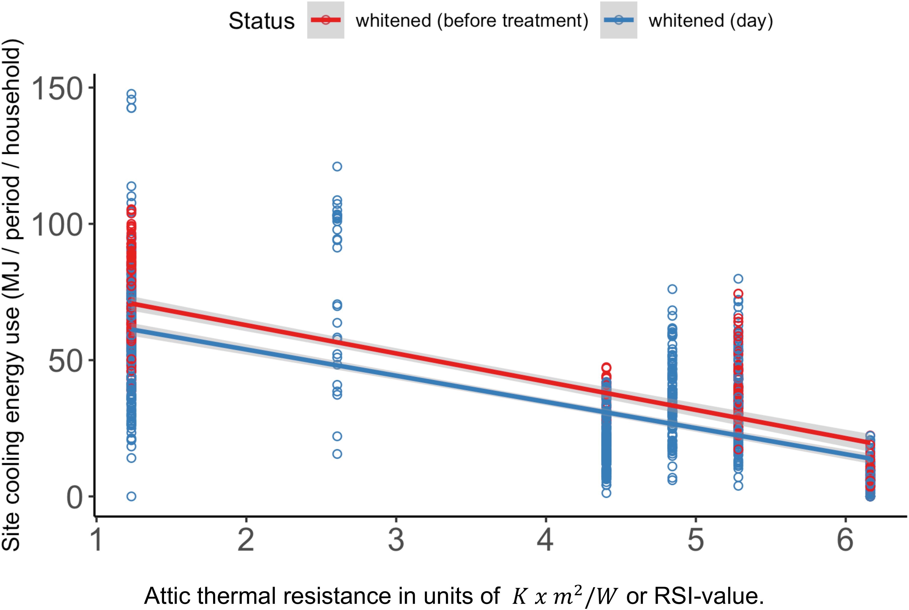
Figure 2. Household-level variation in site cooling energy use given attic insulation and whitening for six treated household. Attic insulation is not reported for one of the seven treated households. Convert the RSI value to an R value (in°F ⋅ ft² ⋅ h/BTU) by multiplying RSI values by 5.68.

FIGURE 3

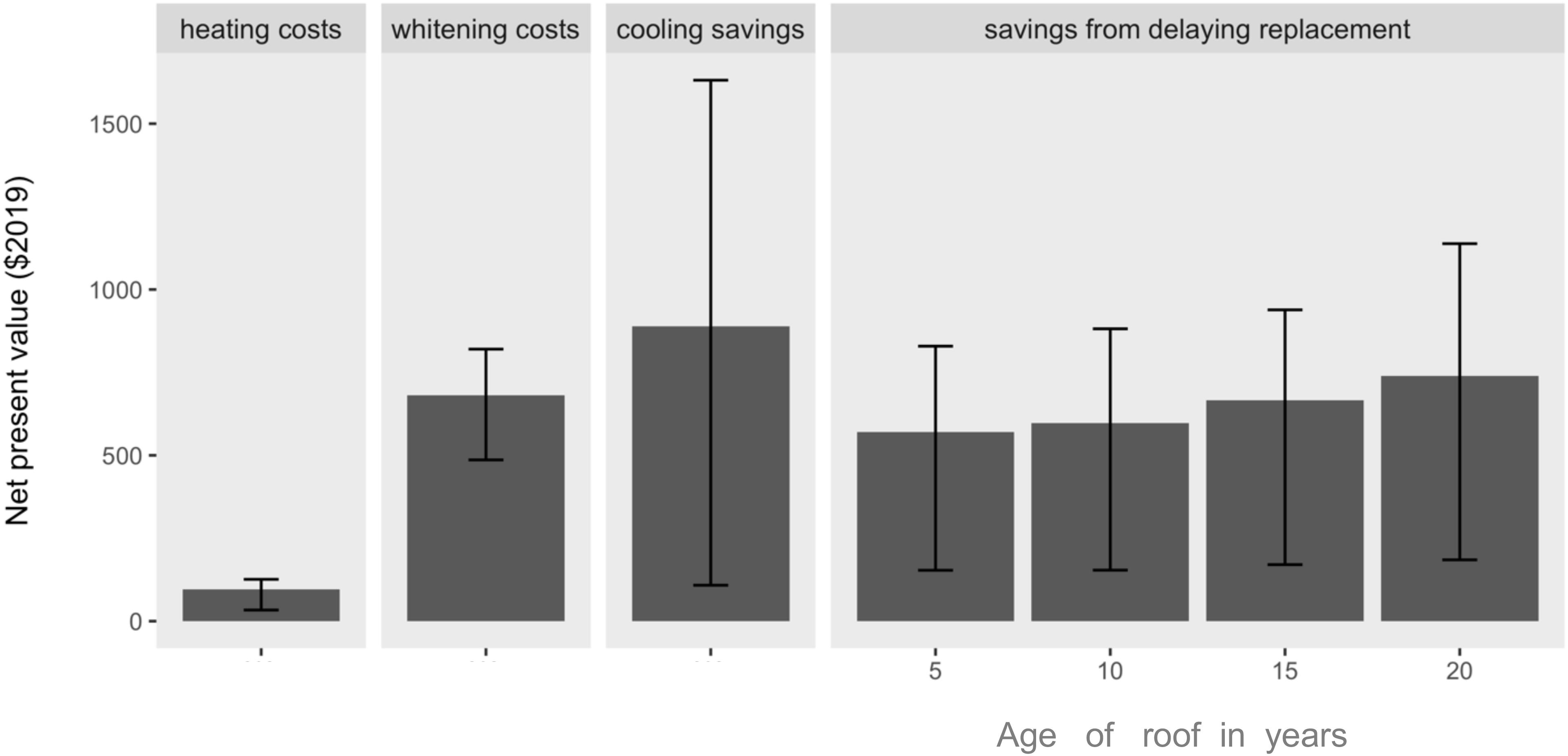
Figure 3. Household net present values for heating penalty, cooling savings, whitening savings, and savings from delaying roof replacement as a result of coating. The ranges include all sources of variability and uncertainty summarized in Table 2 and reflect the first and third quartiles. Results are shown for a discount rate of 5%. Similar results for discount rates of 3% and 7% are included in the Supplementary Information.

There are dozens of household and occupant factors expected to influence air conditioning consumption and the impact of white roofs. Since few, if any, of these factors can be measured in a realistic policy setting, regression is needed to estimate the mean effects, controlling for confounding variation where possible. Table 5 summarizes the two-way fixed effects regression. Both day and night regresses suggest that whitening reduces electricity consumption (β_post < 0). While OLS estimates of β_post demonstrate statistical significance, clustering errors by household to moderate serial correlation increases the standard error of the coefficients to ranges normally not considered significant. The clustered errors should be contextualized given the small, unbalanced sample (MacKinnon and Webb, 2017). Using OLS estimators, the mean reductions in daytime and nighttime site cooling energy use are 7.6% and 1.8%, respectively. These reductions are considerably smaller than the household-level analysis presented in Table 4 because Eq. 2 controls for other sources of variability that might either be improperly attributed to whitening or influence whitening’s impact, such as the example presented with insulation.

TABLE 5

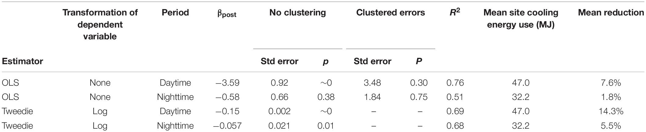
Table 5. Regression results for applying Eq. 2 to the sample.

Relative to OLS estimates, using Tweedie estimators that better accommodate inflated zeros slightly worsens model fit for daytime periods (from a coefficient of determination or R² of 0.76 to 0.69) but improves model fit for nighttime considerably (from an R² of 0.51 to 0.68). This is likely because more homes have more inactive air conditioning periods at night. The Tweedie estimators also increase the impact of whitening from a mean reduction of 7.6% (OLS) to 14.3% (Tweedie) for daytime periods and 1.8% to 5.5% for nighttime site cooling energy use. Tweedie estimates decrease the p values for models of nighttime period from those well above thresholds considered significant (p = 0.38 for OLS estimators) to a p value of 0.01 using Tweedie regression.

Site cooling energy reduction estimates were drawn equally from estimated coefficients (β_post) using both the OLS and Tweedie estimators. Only daytime reductions were assumed, producing a conservatively low estimate of reductions in site cooling energy use.

Figure 3 shows the results for each category of life-cycle costs, including decreased costs for cooling, increased heating costs (the heating penalty), the cost of roof whitening (labor and materials), and the savings from delaying replacement. See Table 2 for assumptions used in the life-cycle cost analysis. Life-cycle results indicate that the savings from delaying replacement are on par with or greater than the other cash flows. Even for relatively new roofs, the benefit from delaying replacement is, on average, more than half of the savings from reduced cooling. For older roofs, the benefit for delaying replacement is similar to that of the cooling savings. Uncertainty in the estimated cooling savings is high because the savings were estimated by drawing from two distributions estimated for the regression coefficient for β_post: one using basic OLS and Tweedie regression.

Figure 4 shows the overall net present value for different assumed roof ages and years of extended roof life (“years replacement delayed”). When adding costs and benefits, costs have been assigned a negative value and benefits have been assigned a positive value such that positive net present values represent a net savings. Absent increasing the service life, whitening would pay for itself in roughly 41% of simulations over the lifetime of the coating with a median cost of $310 and a simple payback period of 22 years. However, including a benefit of delaying roof replacement significantly alters the benefit–cost implications. Across all simulations that assume some increased service life, the median simple payback period and net benefit are 1 year and $310, respectively. The positive benefits of whitening are only robust for older roofs and longer service lives from coating. For example, for roofs older than 10 years of age, most simulations reflect net savings if the coating lasts at least 5 years. This is despite the broad uncertainty in the empirically estimated impact of cooling.

FIGURE 4

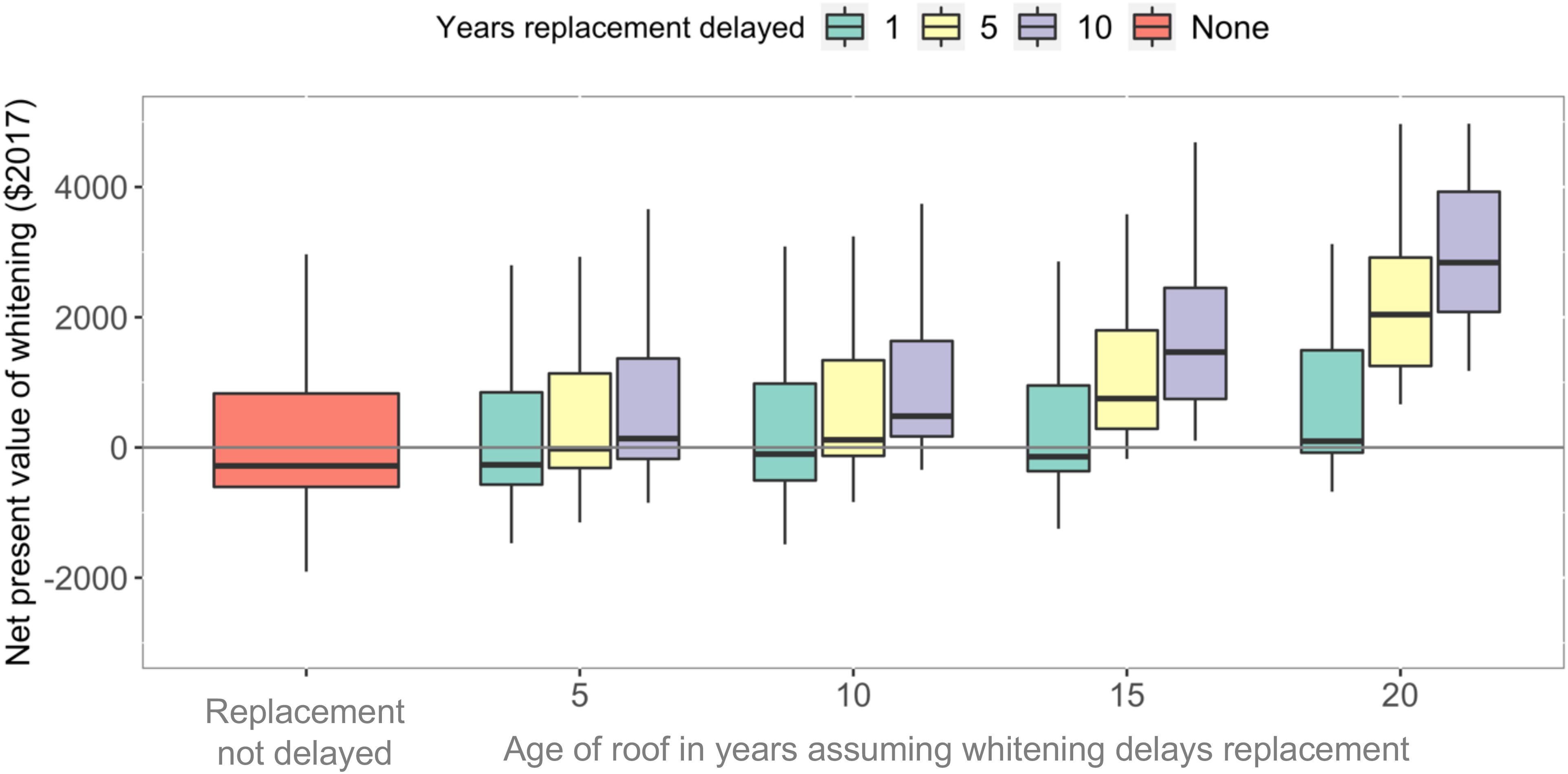
Figure 4. Simulated per household net present values from coating roofs in homes represented by the sample. Positive values reflect a net savings. Results are shown assuming whitening does not delay roof replacement (far left) and does delay replacement for different roof ages. Ranges reflect the first and third quartile values and include uncertainty and variability summarized in Table 2. Results are shown for a discount rate of 5%. Similar results for discount rates of 3% and 7% are included in the Supplementary Information.

Discussion

The potential energy benefits of cool roofs have spurred policies that encourage cool roof choices through incentives and labels. Properly measuring policy performance therefore must extend beyond theoretical models to accommodate unobserved occupant and household heterogeneity that also affects energy consumption. The empirically estimated average reduction in site cooling energy use from roof whitening—ranging from 7.8% to 14.3%—are on par with theoretical results profiled in the section “Introduction.” In particular, these results conform to a recent study that estimates cool roof savings for areas throughout the United States using applied theoretical models (Rosado and Levinson, 2019). Simulations for homes in Houston, TX, United States assuming varied vintages (pre-1980, 1989, and 2012) and orientations (East–West and North–South) estimate mean site cooling energy reductions for two-story homes of 4.7%, which would roughly correspond to 9.4% for a one-story home. While these consistencies between theory and empirical estimates are helpful, more robust empirical evidence than demonstrated here—derived through larger and more diverse samples—is needed to build widespread confidence in whitening’s impact.

The empirical evidence indicating whitening’s effect is limited by the small sample size of treated homes (n = 7). Despite this limitation, the study is demonstrative of empirical methods that can measure cool roof performance in the future, providing an approach that differentiates between daytime and nighttime performance, distinguishing between heating and cooling seasons, modeling of zero inflated data expected of site cooling energy use, and reflecting the potential benefit of delaying roof replacement. The examples provided herein can improve future research and policy making. For example, primary heating data could readily be incorporated into the DiD framework to incorporate the heating penalty in the regression framework. Also, the DiD analysis can flexibly include other covariates, such as geographic factors or orientation, which could be used to study roof performance for a sample that reflect more diverse climates or diverse homes. The methods outlined here would also be beneficial to document expected long-term decline of whitening’s performance.

Future studies could make better use of diurnal variation in cool roofs’ performance, where the treatment effect becomes muted at some point each night. This has the effect of increasing variation in the treatment effect, which both improves statistical rigor and would allow for more explicit testing of the “parallel trend” assumption inherent in DiD. This assumption assumes homogeneous time effects between the treated and control groups outside of the treatment itself (e.g., β₂ in Eq. 1 is the same for both treated and control groups). Experiments that couple monitoring energy consumption alongside roof surface temperatures for treated and control samples would help identify periods in which the treatment effect is muted at night.

The protective nature of cool coating materials is expected to increase the service life of roofs, but the amount of extended service life is uncertain and likely voids any remaining manufacturer warranties. Also, homeowners do not often know when their roof will fail. So, the delayed-replacement benefit of coating acts like a premium to insure against the future risk of failure. It is not clear how homeowners would weigh the potential benefits of delaying replacement given these uncertainties, suggesting an opportunity for future social science research.

Conclusion

The empirical evidence for whitening’s impact on cooling is mixed, with insight primarily constrained by a small treated sample. Most individual household-level comparisons of consumption before and after whitening demonstrate statistically significant (p < 0.01) reductions from 14% to 49.2% during the day. During the nighttime, one house demonstrated a 9.7% increase in site cooling energy use (p = 0.018) with the remaining treated households demonstrating statistically significant (p < 0.01) nighttime reductions ranging from 14% to 40.3%. These results suggest the benefits of cooling extent past sunset, consistent with other observations (Parker and Barkaszi, 1997). Regressions results estimating the mean group effect are also mixed. OLS estimates demonstrate a statistically significant mean daytime reduction of 7.6% but no significant mean nighttime reductions. However, clustering the errors by household to moderate serial correlation increases p values to levels usually considered insignificant. Tweedie regressions, which better fit the slight zero inflation demonstrated in the sample, improve the model fit for nighttime consumption and produce statistically significant air conditioning reductions of 14.3% and 5.5% during the day and night, respectively.

The benefit for delaying roof replacement was found to be on par with or greater than other more conventionally estimated costs and benefits. A 5-year delay in roof replacement sways the average benefits of whitening to nearly negligible to quite favorable for roofs older than 10 years of age, results generally robust to a range of assumptions.

Data Availability Statement

Pecan Street Inc. provides to researchers the raw data supporting the conclusions of this article.

Author Contributions

MB performed all of the analysis and wrote the manuscript independently.

Funding

This work was supported by the Moses Feldman Family Foundation.

Conflict of Interest

The authors declare that the research was conducted in the absence of any commercial or financial relationships that could be construed as a potential conflict of interest.

Acknowledgments

The author would also like to thank the Pecan Street Research Institute for their ongoing commitment to publishing world-class building energy and water demand data, Colin Clark for his vision for and commitment to this work, and Dr. Randy Walsh for his helpful comments on the modeling and manuscript.

Supplementary Material

The Supplementary Material for this article can be found online at: https://www.frontiersin.org/articles/10.3389/fbuil.2020.571429/full#supplementary-material

References

Adan, H., and Fuerst, F. (2016). Do energy efficiency measures really reduce household energy consumption? A difference-in-difference analysis. Energy Effic. 9, 1207–1219. doi: 10.1007/s12053-015-9418-3

CrossRef Full Text | Google Scholar

Adland, R., Cariou, P., Jia, H., and Wolff, F.-C. (2018). The energy efficiency effects of periodic ship hull cleaning. J. Clean. Prod. 178, 1–13. doi: 10.1016/j.jclepro.2017.12.247

CrossRef Full Text | Google Scholar

Akbari, H., and Konopacki, S. J. (1998). “The impact of reflectivity and emissivity of roofs on building cooling and heating energy use,” in Proceedings of Thermal VII: Thermal Performance of the Exterior Envelopes of Buildings VII, (Florida, FL: ASHRAE). doi: 10.1080/17512549.2014.890541

CrossRef Full Text | Google Scholar

Al-Obaidi, K. M., Ismail, M., and Abdul Rahman, A. M. (2014). Passive cooling techniques through reflective and radiative roofs in tropical houses in southeast asia: a literature review. Front. Archit. Res. 3, 283–297. doi: 10.1016/j.foar.2014.06.002

CrossRef Full Text | Google Scholar

APOC (2017). Energy Efficient Cool Roof Coatings. Available Online at: https://www.apoc.com/pages/energy-efficiency (accessed December 21, 2017).

Google Scholar

Austin Energy (2013). City of Austin, Texas, “Residential Electric Rates & Line Items. Texas: Austin Energy. Available Online at: https://austinenergy.com/ae/rates/residential-rates/residential-electric-rates-and-line-items (accessed June 27, 2017).

Google Scholar

BEHR (2020). Multi-Surface Roof Paints for Your Project. Available Online at: https://www.behr.com/consumer/products/specialty-paint/roof-paint/behr-multi-surface-roof-paint (accessed September 10, 2020)

Google Scholar

Bertrand, M., Duflo, E., and Mullainathan, S. (2004). How much should we trust differences-in-differences estimates? Q. J. Econ. 119, 249–275. doi: 10.1162/003355304772839588

PubMed Abstract | CrossRef Full Text | Google Scholar

Brito Filho, J. P., and Santos, T. V. O. (2014). Thermal analysis of roofs with thermal insulation layer and reflective coatings in subtropical and equatorial climate regions in brazil. Energy Build. 84, 466–474. doi: 10.1016/j.enbuild.2014.08.042

CrossRef Full Text | Google Scholar

Cool Roof Rating Council (2017). Resources – Rebates & Codes – Cool Roof Rating Council. Available Online at: http://coolroofs.org/resources/rebates-and-codes (accessed July 07, 2017)

Google Scholar

R Core Team (2020). R: A language and environment for statistical computing. Vienna: R Foundation for Statistical Computing.

Google Scholar

Damodaran, A. (2017). Total return on 10-year government bonds, price changes imputed from yields. Available Online at: http://pages.stern.nyu.edu/~adamodar/New_Home_Page/datafile/histretSP.html (accessed December 19, 2017).

Google Scholar

Datta, S., and Filippini, M. (2016). Analysing the impact of ENERGY STAR rebate policies in the US. Energy Effic. 9, 677–698. doi: 10.1007/s12053-015-9386-7

CrossRef Full Text | Google Scholar

de Brito Filho, J. P., Henriquez, J. R., and Dutra, J. C. C. (2011). Effects of coefficients of solar reflectivity and infrared emissivity on the temperature and heat flux of horizontal flat roofs of artificially conditioned nonresidential buildings. Energy Build. 43, 440–445. doi: 10.1016/j.enbuild.2010.10.007

CrossRef Full Text | Google Scholar

Doe (U.S. Department of Energy) (2012). Residential Energy Consumption Survey, 2009,” U.S. Department of Energy, Energy Information Administration (EIA). Washington, D.C: DOE (U.S. Department of Energy).

Google Scholar

Doe (U.S. Department of Energy) (2017a). Cool Roofs. Washington, D.C: DOE (U.S. Department of Energy).

Google Scholar

Doe (U.S. Department of Energy) (2017b). Residential Energy Consumption Survey, 2015,” U.S. Department of Energy, Energy Information Administration (EIA). Washington, D.C: DOE (U.S. Department of Energy).

Google Scholar

Doe (U.S. Department of Energy) (2017c). U.S. Natural Gas Prices. Washington, D.C: DOE (U.S. Department of Energy).

Google Scholar

Energy Star (2017). Energy Efficient Roofing Products. Taiwan: Energy Star. Available Online at: https://www.energystar.gov/products/building_products/roof_products

Google Scholar

Goodman-Bacon, A. (2018). Difference-in-differences with variation in treatment timing. Cambridge: National Bureau of Economic Research.

Google Scholar

Hernández-Pérez, I., Álvarez, G., Xamán, J., Zavala-Guillén, I., Arce, J., and Simá, E. (2014). Thermal performance of reflective materials applied to exterior building components-A review. Energy Build. 80, 81–105. doi: 10.1016/j.enbuild.2014.05.008

CrossRef Full Text | Google Scholar

homeadvisor.com (2017). 2017 Roof Repair Costs. Average Price to Fix a Roof. Available Online at: http://www.homeadvisor.com/cost/roofing/repair-a-roof/ (accessed June 23, 2017).

Google Scholar

homewyse.com (2017). Cost to Paint Home – 2017 Cost Calculator (Customizable). Available Online at: https://www.homewyse.com/services/cost_to_paint_home.html (accessed December 19, 2017).

Google Scholar

Hosseini, M., and Akbari, H. (2014). Heating energy penalties of cool roofs: the effect of snow accumulation on roofs. Adv. Build. Energy Res. 8, 1–13.

Google Scholar

Levinson, R., and Akbari, H. (2010). Potential benefits of cool roofs on commercial buildings: conserving energy, saving money, and reducing emission of greenhouse gases and air pollutants. Energy Effic. 3:5. doi: 10.1007/s12053-008-9038-2

CrossRef Full Text | Google Scholar

Levinson, R., Akbari, H., Konopacki, S., and Bretz, S. (2005). Inclusion of cool roofs in nonresidential title 24 prescriptive requirements. Energy Policy 33, 151–170. doi: 10.1016/S0301-4215(03)00206-4

CrossRef Full Text | Google Scholar

Levinson, R., Gilbert, H., Long, Y., Slack, J., Ban-Weiss, G., Goudey, H., et al. (2019). Solar-Reflective ‘Cool’ Walls: Benefits, Technologies, and Implementation. Appendix P: Cool Wall Application Guidelines,” California Energy Commission, CEC-500-2019-040. Sacramento: California Energy Commission. Available Online at: http://dx.doi.org/10.20357/B7SP4H

Google Scholar

MacKinnon, J. G., and Webb, M. D. (2017). Wild bootstrap inference for wildly different cluster sizes. J. Appl. Econom. 32, 233–254. doi: 10.1002/jae.2508

CrossRef Full Text | Google Scholar

Nahar, N. M., Sharma, P., and Purohit, M. M. (2003). Performance of different passive techniques for cooling of buildings in arid regions. Build. Environ. 38, 109–116. doi: 10.1016/S0360-1323(02)00029-X

CrossRef Full Text | Google Scholar

Navy, U. S. (2017). Sun or Moon Rise/Set Table for One Year. Available Online at: http://aa.usno.navy.mil/data/docs/RS_OneYear.php (accessed June 21, 2017)

Google Scholar

New, J., Miller, W. A., (Joe) Huang, Y., and Levinson, R. (2016). Comparison of software models for energy savings from cool roofs. Energy Build. 114, 130–135. doi: 10.1016/j.enbuild.2015.06.020

CrossRef Full Text | Google Scholar

Parker, D. S., and Barkaszi, S. F. (1997). Roof solar reflectance and cooling energy use: field research results from Florida. Energy Build. 25, 105–115. doi: 10.1016/S0378-7788(96)01000-6

CrossRef Full Text | Google Scholar

Pecan Street Research Institute (2017). Dataport. Los Angeles: Pecan Street. Available Online at: https://www.pecanstreet.org/dataport/

Google Scholar

Pisello, A. L., Piselli, C., and Cotana, F. (2015). Influence of human behavior on cool roof effect for summer cooling. Build. Environ. 88, 116–128. doi: 10.1016/j.buildenv.2014.09.025

CrossRef Full Text | Google Scholar

Rosado, P. J., and Levinson, R. (2019). Potential benefits of cool walls on residential and commercial buildings across California and the United States: conserving energy, saving money, and reducing emission of greenhouse gases and air pollutants. Energy Build. 199, 588–607. doi: 10.1016/j.enbuild.2019.02.028

CrossRef Full Text | Google Scholar

Sproul, J., Wan, M. P., Mandel, B. H., and Rosenfeld, A. H. (2014). Economic comparison of white, green, and black flat roofs in the United States. Energy Build. 71, 20–27. doi: 10.1016/j.enbuild.2013.11.058

CrossRef Full Text | Google Scholar

Synnefa, A., Santamouris, M., and Akbari, H. (2007). Estimating the effect of using cool coatings on energy loads and thermal comfort in residential buildings in various climatic conditions. Energy Build. 39, 1167–1174. doi: 10.1016/j.enbuild.2007.01.004

CrossRef Full Text | Google Scholar

Wickham, H. (2016). ggplot2: Elegant Graphics for Data Analysis. New York: Springer-Verlag.

Google Scholar

Wickham, H., François, R., Henry, L., and Müller, K. (2020). dplyr: A Grammar of Data Manipulation, R package version 1.0.2.

Google Scholar