Machine Learning for Extracting Features of Approximate Optimal Brace Locations for Steel Frames

Introduction

The optimization problem of brace locations on a plane frame is a standard problem that has been extensively studied over the past few decades (Ohsaki 2010). However, it is categorized as a topology optimization problem that involves integer variables indicating the existence/nonexistence of members. Therefore, it is more difficult than a sizing optimization problem, where the cross-sectional properties are considered as continuous design variables and their optimal values are found using a nonlinear programming algorithm. Furthermore, another difficulty exists in the problem with stress constraints (Senhola et al., 2020), which are to be satisfied by only existing members; therefore, the constraints are design-dependent, and the problem becomes a complex combinatorial optimization problem.

The solution methods for combinatorial optimization problems are categorized into mathematical programming and heuristic approaches. For a truss structure, the topology optimization problem with stress constraints can be formulated as a mixed-integer linear programming (MILP) problem (Kanno and Guo, 2010). However, the computational cost for solving an MILP problem is very large, even for a small-scale truss. By contrast, various heuristic methods, including genetic algorithms, simulated annealing (Aarts and Korst, 1989), tabu search (Glover, 1989), and particle swarm optimization (Kennedy and Eberhart, 1995), have been proposed for topology optimization problems (Saka and Geem, 2013). Hagishita and Ohsaki (2008a) proposed a method based on the scatter search. Some methods have been proposed for generating brace locations using the technique of continuum topology optimization (Rahmatalla and Swan, 2003; Beghini et al., 2014). However, the computational cost of a heuristic approach is also very large for a structure with many nodes and members. Therefore, the computational cost may be substantially reduced if a solution that cannot be an approximate optimal solution or a feasible solution is excluded before carrying out structural analysis. For this purpose, machine learning can be effectively used.

Machine learning is a basic process of artificial intelligence, the use of which has resulted in great successes in the field of pattern recognition (Carmona et al., 2012). Support vector machine (SVM) (Cristianini and Shawe-Taylor, 2000), artificial neural network (ANN) (Adeli, 2001), and binary decision tree (BDT), are regarded as the most popular methods. The application of machine learning to the solution process of optimization problems has been studied by many researchers, including Szczepanik et al. (1996) and Turan and Philip (2012). Probabilistic models, including Bayesian inference, Gaussian process model (Okazaki et al., 2020), and Gaussian mixture model (Do and Ohsaki, 2020), have also been extensively studied.

The application of machine learning to structural response analysis and structural optimization has been studied since the 1990s in conjunction with data mining approaches (Hagishita and Ohsaki, 2008b; Witten et al., 2011). The use of machine learning is categorized into several levels. The simplest level is to estimate the structural responses that are to be obtained by complex nonlinear and/or dynamic analysis, demanding a large computational cost. For example, SVM for regression (Smola and Schölkopf, 2004; Luo and Paal, 2019) has successfully been applied to reliability analysis (Li et al., 2006; Liu et al., 2017b; Dai and Cao, 2017), and ANN (Papadrakakis et al., 1998; Panakkat and Adeli, 2009), including deep neural network (DNN) (Nabian and Meidani, 2018; Yu et al., 2019), can be used for estimating multiple response values. Nguyen et al. (2019) used DNN for predicting the strength of a concrete material. Abueidda et al. (2020) used DNN for finding the optimal topology of a plate with material nonlinearity. The approaches in this level are regarded as surrogate or regression models which are similar to the conventional methods of response surface approximation, Gaussian process model, etc. (Kim and Boukouvala., 2020). Most of the research on machine learning for structural optimization are classified into this level. The computational cost for structural analysis during the optimization process can be drastically reduced using machine learning for constructing a surrogate model.

The second-level application of machine learning to structural optimization may be to classify the solutions into two groups, such as feasible and infeasible solutions or approximate optimal and non-optimal solutions. During the optimization process using a heuristic method, the solutions judged as infeasible or non-optimal can be simply discarded without carrying out structural analysis. Cang et al. (2019) applied machine learning to an optimization method using the optimality criteria approach. Liu et al. (2017a) used clustering for classifying the solutions. Kallioras et al. (2020) used deep belief network for accelerating the topology optimization process. Various methods of data mining can be used for classifying the solutions; however, the number of studies included in this level is rather small. In this paper, we extend the method using SVM in our previous paper (Tamura et al., 2018) to classify the brace types and locations of a large-scale frame.

The most advanced use of machine learning in structural optimization may be to directly find the optimal solution without resorting to an optimization algorithm. Several approaches have been proposed for learning the properties of optimal solutions of plates subjected to in-plane loads (Lei et al., 2018). However, it is difficult to estimate the properties of optimal solutions with enough precision so as to find the optimal solutions without using an optimization algorithm. Alternatively, reinforcement learning may be used for training an agent, simulating the decision-making process of an expert (Yonekura and Hattori, 2019; Hayashi and Ohsaki, 2020a, Hayashi and Ohsaki, 2020b).

One of the drawbacks in the application of machine learning to structural optimization is that the computational cost for generating the sample dataset for learning and the process of learning itself may exceed the reduction of the computational cost for optimization by utilizing the learning results. Therefore, it is important to develop a method such that the machine learning results of a small-scale model can be utilized for extracting the features of approximate optimal and non-optimal solutions of a large-scale model. Furthermore, it is beneficial and intuitive to structural designers and engineers if the important features or properties observed in the approximate optimal solutions can be naturally extracted by the machine learning process. However, it is well known that the learning results by ANN are not interpretable. Although feature selection is an established field of research in machine learning, its main purpose is the reduction of the number of features (input variables) to prevent overfitting and reduce the computational cost in the learning process (Xiong et al., 2005; Abe, 2007; Stańczyk and Jain, 2015).

Identification of important features is very helpful for finding a reasonable distribution of braces preventing unfavorable yielding under strong seismic motions. A building frame should also be appropriately designed for preventing collapse due to unfavorable deformation concentration (Bai et al., 2017), which can be enhanced by the P-delta effect (Kim et al., 2009). However, the seismic load considered in this paper is of a level of moderately strong motion (level 2 in the Japanese building code); we do not consider a critically strong motion (level 3 in the Japanese building code) that would lead to a collapse due to deformation concentration.

In this paper, we present a method for extracting the important features of brace types and locations of approximate optimal large-scale steel building frames subjected to static seismic loads utilizing the machine learning results of a small-scale model. The maximum stress in the members, including beams, columns, and braces, is to be minimized under constraints on the number of braces in each story and the maximum interstory drift angle among all stories. The key points of this study are summarized as follows:

• A new formulation is presented for identifying important features of the solutions with large score values from the machine learning results by SVM with radial basis function (RBF) kernel.

• A method is presented to estimate important features of a large-scale model from the machine learning results of a small-scale frame.

• The important features of brace types and locations of an approximate optimal 24-story frame can be successfully extracted using the machine learning results of a 12-story frame. A clear difference exists in the cumulative numbers of appearance of important features in the approximate optimal solutions and the non-optimal solutions.

Optimization Problem

Consider an $n_f$-story $n_s$-span plane steel frame. An example of a12-story 4-span frame is shown in Figure 1. The types and locations of braces are optimized to minimize the maximum absolute value of the edge stress in members, including beams, columns, and braces, under static horizontal loads representing the seismic loads. The vertical loads are not considered, assuming the process of seismic retrofit installing various types of braces to a frame consisting of beams and columns (Tamura et al., 2018) (i.e., the braces do not have any stress under vertical loads).

FIGURE 1

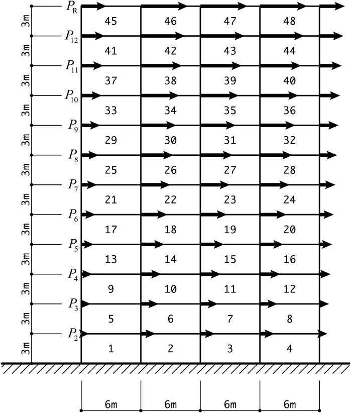
FIGURE 1. A 12-story 4-span frame.

The braces are selected from the $n_b$ types, including “no-brace”. The five types in Figure 2 are used in the numerical examples. These types are identified by the integer variable $t_i\in \{\mathrm{1,2},\dots ,n_b\}$, where the index $i=1,\dots ,n_f{n}_s$ indicates the location in which a brace can be installed. For the 12-story 4-span frame, there are 48 locations, as indicated in Figure 1. As is well known, the types and locations of braces have significant influence on the stresses in beams, columns, and braces. Continuously located braces will transmit the horizontal seismic loads smoothly to the supports, while discontinuous braces will cause excessive axial forces and bending moments in the members. Therefore, it is possible to investigate efficient locations of braces using a machine learning method.

FIGURE 2

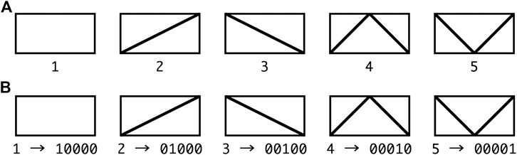
FIGURE 2. Types of braces including “no-brace”; (A) categorical variable, 1) no-brace, 2) right diagonal brace, 3) left diagonal brace, 4) K-brace, 5) V-brace, (B) binary representation of brace types.

Among the various methods of machine learning, we use SVM to extract important features of brace types and locations. We can investigate the properties of approximate optimal solutions using SVM more easily than ANN, for which the learning results are difficult to interpret. SVM is effective for ordered input feature values. However, in our problem, the types $\mathrm{1,2},\dots ,n_b(=5)$ in Figure 2A do not have any order in view of the effect on the structural responses, i.e., $t_i$ is a categorical variable, which should be converted into a set of dummy variables (Tamura et al., 2018). For this purpose, a binary variable $x_{ij}$ is introduced for each type of brace so that $x_{ij}=1$ if $t_i=j$, otherwise $x_{ij}=0$, as shown in Figure 2B. In the vector consisting of $m=n_b{n}_f{n}_s$ binary variables, $x_{ij}$ is denoted by $x$.

It is possible to express the ‘no-brace’ by $x_{i2}=x_{i3}=\cdots =x_{i{n}_b}=0$ without using the variable $x_{i1}=1$. Accordingly, the representation using $n_{\text{b}}$ binary variables $x_{i1},\dots ,x_{i{n}_b}$ for each brace location has a redundancy, which is called multicollinearity, and should be prevented in a multivariate analysis. However, it is known that multicollinearity does not cause any serious problems for SVM, because unnecessary features are automatically ignored in the learning process. It has been confirmed by Tamura et al. (2018) that the representation with five binary variables in Figure 2 has better performance than that with four variables and without “no-brace”.

Let ${\sigma }_i\left(x\right)$ denote the maximum absolute value of the edge stresses of member i which may be a beam, a column, or a brace. We minimize the maximum value of ${\sigma }_i\left(x\right)$ among $n_m$ members, which is called maximum stress for brevity. However, it is difficult to determine the optimal locations of braces that have relatively small absolute values of stress, if only the maximum stress among all members is to be considered in the objective function. Therefore, we use the following p-norm to incorporate the effect of brace locations that are not directly related to the maximum stress:

$F\left(x\right)={\left[{\displaystyle \sum _{i=1}^{n_m}{\left({\sigma }_i\left(x\right)\right)}^p}\right]}^{\frac{1}{p}}(1)$

A constraint is given for the number of braces $n_i^b$ in the ith story, which should be equal to ${\overline{n}}^b$. To prevent selecting a too flexible structure against seismic loads as a candidate of approximate optimal solution, an upper bound $\overline{r}$ is assigned to the maximum interstory drift angle $r_{\max }\left(x\right)$ among all stories. Then, the optimization problem is formulated as

$\begin{array}{l}MinimizeF\left(x\right)={\left[{\displaystyle \sum _{i=1}^{n_m}{\left({\sigma }_i\left(x\right)\right)}^p}\right]}^{\frac{1}{p}}\\ subjectto{n}_i^b={\overline{n}}^b,\left(i=\mathrm{1,2},\dots ,n_f\right)\\ r_{\max }\left(x\right)\le \overline{r}\end{array}(2)$

Outline of Machine Learning Using SVM

Tamura et al. (2018) showed that the approximate optimal solutions, which have objective function values close to the optimal value, and the non-optimal solutions, which cannot be the optimal solution, can be classified for a small 5-story 3-span frame using SVM and BDT. They demonstrated that the optimization process using SA can be accelerated utilizing the machine learning results so that structural analysis is carried out only for the neighborhood solutions labeled as approximate optimal. In their method, a dataset of 10,000 samples (pairs of the design variables and the corresponding objective function value) is randomly generated for training, and the 1,000 (10%) best and the 1,000 (10%) worst solutions are regarded as approximate optimal and non-optimal solutions, respectively, which are labeled as $y=1$ and $y=-1$. However, it is not realistic to carry out machine learning for each frame mode to be optimized, because the computational cost for preparing the dataset and the learning process will be too large even though a substantial reduction of the computational cost is expected for the optimization process. Therefore, in this paper, we present a method for utilizing the machine learning results of a small-scale frame to evaluate the properties of a large-scale frame, where SVM is used as the machine learning tool. The complex data that cannot be classified using the linear kernel can be successfully classified using nonlinear kernels such as polynomial and RBF kernels. The details of SVM are not explained here, because they are available in textbooks such as Cristianini and Shawe-Taylor (2000).

Suppose the learning process is completed using a set of n samples $\left[\left(x_1,y_1\right),\dots ,\left(x_n,y_n\right)\right]$ of design variable (input) vector $x_i$ and the response (output) value $y_i$. The score $S\left(x\right)$ of a variable vector x is computed, as follows, using the kernel function $K(x_i,x)$, coefficients ${\alpha }_i^{\ast }$, and bias $b^{\ast }$:

$S\left(x\right)={\displaystyle \sum _{i=1}^n\left[y_i{\alpha }_i^{\ast }K\left(x_i,x\right)\right]}+b^{\ast }(3)$

The value of y of a variable vector x is estimated from $S\left(x\right)$ as

$y=\{\begin{array}{c}1ifS\left(x\right)\ge 0\\ -1ifS\left(x\right)<0\end{array}(4)$

Accuracy of the machine learning results is generally quantified by the ratios of TP (true positive) and TN (true negative), for which the labels $y=1$ and $-1$ are estimated correctly, and FP (false positive) and FN (false negative), for which the labels $y=-1$ and 1 are estimated wrongly as $y=1$ and $-1$, respectively. For application of the machine learning results to find the optimal solution of problem Eq. 2, the ratio of FN should be reduced so that a candidate of the optimal solution is not missed during the optimization process, while structural analysis is not carried out for a solution estimated as $y=-1$. Reducing the ratio of FP is also important to reduce the computational cost for optimization.

In the following numerical examples, we use the function fitcsvm in the Statistics and Machine Learning Toolbox of MATLAB R2016b (MathWorks, 2016). The kernel scaling factor is assigned automatically, and the appropriate value of the box constraint parameter is investigated in Properties of Small-Scale Frame Section.

Identification of Important Features

One of the drawbacks of machine learning using, for example, ANN, is that understanding the reasons for the obtained results is very difficult. In other words, identification of important features in the input variable vector is very difficult. In this section, we present a method for extracting the important features contributing to a large score value using SVM. In our problem, the feature corresponds to the component of x representing the type of brace, including “no-brace”, to be assigned at each location in the frame.

If the linear kernel is used, the score function of a variable vector x is evaluated as

$S\left(x\right)={\displaystyle \sum _{i=1}^n{y}_i{\alpha }_i{x}_i^{T}x}+b(5)$

where ${\alpha }_i$ and $b$ are the coefficients and the bias identified by machine learning, respectively, and $x_i$ is the ith sample in the training dataset. Using the parameter vector $\beta =({\beta }_1,\dots ,{\beta }_m)$ defined as

$\beta ={\displaystyle \sum _{i=1}^n{y}_i{\alpha }_i{x}_i}(6)$

the score $S\left(x\right)$ can be rewritten as

$S\left(x\right)={\beta }^{T}x+b={\displaystyle \sum _{j=1}^m{\beta }_j{x}_j}+b(7)$

Hence, contribution of the feature $x_j$ is estimated by the value of weight coefficient ${\beta }_j$. Suppose the set of jth feature $\{x_{1j},\dots ,x_{nj}\}$, i.e., the jth components $x_{ij}$ of $x_1,\dots ,x_n$, has the mean value ${\mu }_j$ and the standard deviation ${\delta }_j$ among all samples. Then, the jth components $x_{ij}$ and $x_j$ of the vectors $x_i$ and x, respectively, are normalized to ${\widehat{x}}_{ij}$ and ${\widehat{x}}_j$ as

${\widehat{x}}_{ij}=\frac{x_{ij}-{\mu }_j}{{\delta }_j},{\widehat{x}}_j=\frac{x_j-{\mu }_j}{{\delta }_j}(8)$

so that the mean value and the standard deviation are equal to 0 and 1, respectively. The vectors consisting of ${\widehat{x}}_{ij}$ and ${\widehat{x}}_j$ are denoted by ${\widehat{x}}_i$ and $\widehat{x}$, respectively. The normalized values of $x_j=1$ and 0 expressing existence and non-existence of the specific brace type are denoted as ${\xi }_j^1=(1-{\mu }_j)/{\delta }_j$ and ${\xi }_j^0=(0-{\mu }_j)/{\delta }_j$, respectively. The difference $\Delta S_j\left(x\right)$ between the score values corresponding to $x_j=1$ and 0, while the remaining variables $x_k$$(k\ne j)$ are fixed, is computed as

$\Delta S_j\left(\widehat{x}\right)={\beta }_j({\xi }_j^1-{\xi }_j^0)=\frac{{\beta }_j}{{\delta }_j}(9)$

We can see from Eq. 9 that $x_i=1$ contributes to a larger/smaller score value if ${\beta }_j/{\delta }_j$ is positive/negative.

However, when the nonlinear RBF kernel is used, it is not possible to derive an explicit formulation like Eq. 9, and the score function has a complex form using the normalized feature vector as follows:

$\begin{array}{c}S\left(\widehat{x}\right)={\displaystyle \sum _{i=1}^n\left[y_i{\alpha }_i\exp \left(-\gamma {\Vert {\widehat{x}}_i-\widehat{x}\Vert }^2\right)\right]}+b\\ ={\displaystyle \sum _{i=1}^n\left[y_i{\alpha }_i{\displaystyle \prod _{j=1}^m\exp \left(-\gamma {({\widehat{x}}_{ij}-{\widehat{x}}_j)}^2\right)}\right]}+b\end{array}(10)$

where $\gamma$ is the multiplier for the RBF kernel.

Several methods have been proposed for extracting the important features from the results of SVM using nonlinear kernels (Xiong et al., 2005; Abe, 2007; Stańczyk and Jain, 2015). However, their purpose is the reduction of the number of feature variables to reduce the computational cost for learning, and it is difficult to identify the important features that have a large contribution to the classification of the solutions into the specific groups. Therefore, we propose a simple method below.

Define $c_{ij}$ and $d_{ij}$ as

$\begin{array}{c}{c}_{ij}={\displaystyle \prod _{k\ne j}\exp \left(-\gamma {({\widehat{x}}_{ik}-{\widehat{x}}_k)}^2\right)}\\ d_{ij}=y_i{\alpha }_i\left[\exp \left(-\gamma {({\widehat{x}}_{ij}-{\xi }_j^1)}^2\right)-\exp \left(-\gamma {({\widehat{x}}_{ij}-{\xi }_j^0)}^2\right)\right]\end{array}(11)$

From Eqs 10, 11, the difference of the score values between $x_{ij}=1$ and 0 is computed as

$\Delta S_j\left(\widehat{x}\right)={\displaystyle \sum _{i=1}^n{d}_{ij}{c}_{ij}}(12)$

Let $I_{\text{SV}}$ denote the set of indices of support vectors in the training dataset after the learning process is completed. Then ${\alpha }_i=0$ for $i\notin I_{\text{SV}}$, and accordingly, $d_{ij}=0$ is satisfied for $i\notin I_{\text{SV}}$ in Eq. 12. Furthermore, since ${\widehat{x}}_{ik}$ and ${\widehat{x}}_k$ are the random variables with the same mean and variance, we assume that $c_{ij}$ has almost the same value irrespective of i and j. Validity of this assumption is discussed in Properties of Small-Scale Frame Section. Hence, the effect of existence of the jth feature, i.e., $x_j=1$ is evaluated by

$\Delta {\widehat{S}}_j\left(\widehat{x}\right)={\displaystyle \sum _{i\in I_{SV}}{d}_{ij}}(13)$

Feature Extraction of Large-Scale Frame

When optimizing a large-scale frame, computational cost may be reduced if the machine learning results of a small-scale frame can be utilized. Suppose we carry out machine learning for an $n_{\text{f}1}$-story frame and apply the results to an $n_{\text{f}2}$-story frame $(n_{\text{f}2}\gg n_{\text{f}1})$. For this purpose, the feature values of the $n_{\text{f}1}$-story frame should be expressed as functions of the feature values of the $n_{\text{f}2}$-story frame, for which the score value is to be predicted. These two frames are assumed to have the same $n_{\text{s}}$-span, for simplicity, and the feature values in each span of the $n_{\text{f}2}$-story frame are converted into those in the corresponding span of the $n_{\text{f}1}$-story frame, i.e., the feature values are condensed in the story (height) direction using the same rule for all spans. Furthermore, the same rule is used for all types of braces.

The algorithm for the $n_{\text{f}2}$-story frame utilizing the results of $n_{\text{f}1}$-story frame is summarized as follows:

Step 1. Assemble the feature values in each span of the $n_{\text{f}2}$-story frame into an $n_{\text{f}2}\times n_{\text{b}}$ matrix $X^{n_{f2}}$, where each row corresponds to the story, and each column corresponds to one of the binary variables representing the $n_{\text{b}}$ types of braces including “no-brace”.

Step 2. Compute the $n_{\text{f}1}\times n_{\text{b}}$ matrix $X^{n_{f1}}$ for each span of the $n_{\text{f}1}$-story frame using an $n_{\text{f}1}\times n_{f2}$ matrix $H$ as

$X^{n_{f1}}=H{X}^{n_{f2}}(14)$

Step 3. Obtain the feature vector $x$ of the $n_{\text{f}1}$-story frame by rearranging the components of $X^{n_{f1}}$, and compute the score function value $S\left(x\right)$ using the machine learning results of the $n_{\text{f}1}$-story frame.

Figure 3A illustrates the coding of the matrix $X^{n_{f2}}$ for a single span of a 4-story frame. For example, the 1st row of $X^{n_{f2}}$ corresponds to the 1st story of the frame, and the existence of K-brace corresponds to the vector (0, 0, 0, 1, 0) as defined in Figure 2B. Figure 3B illustrates the condensation process from a 4-story frame to a 2-story frame. If the matrix $H$ is assigned as shown in the figure, the mean values of (1st, 2nd) and (3rd, 4th) stories of the 4-story frame is assigned to the 1st and 2nd stories, respectively, of the 2-story frame (i.e., this process is regarded as a kind of mean—value pooling in the vertical direction).

FIGURE 3

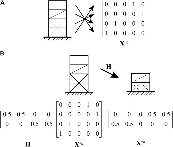
FIGURE 3. Illustration of the condensation process; (A) example of $X^{n_{f2}}$ for a 4-story 1-span frame, (B) condensation from 4-story frame to 2-story frame.

The $\left(i,j\right)$-component of $H$ is regarded as the weight coefficient of the feature value of the jth story of the $n_{\text{f}2}$-story frame to that of the ith story of the $n_{\text{f}1}$-story frame. The converted feature vector reassembled from the matrix $X^{n_{f1}}$ is incorporated into Eq. 10 after normalization using Eq. 8, where the coefficients ${\alpha }_i$ and bias $b$ have been determined by carrying out machine learning for the $n_{\text{f}1}$-story frame. However, the bias $b$ in Eq. 10 should be modified for more accurate prediction results. Therefore, the components of coefficient matrix $H$, as well as the bias $b$, are determined so that the prediction error of the $n_{\text{f}2}$-story frame is minimized.

Let $R$ denote the correlation coefficient between the maximum stress of the large-scale $n_{\text{f}2}$-story frame and the score estimated by the small-scale $n_{\text{f}1}$-story frame. The negative correlation coefficient $R$ is to be minimized because a large score value should correspond to a small value of maximum stress. However, the bias $b$ cannot be determined by minimization of $R$. Furthermore, it is preferable to have small ratios of FP and FN. Therefore, the following problem is to be solved to obtain the values of $H$ and $b$:

$\begin{array}{l}MinimizeG(H,b)=R(H,b)+\frac{w}{{\left({\delta }_S\right)}^2}{\displaystyle \sum _{i\in I_{FN}\cup I_{FP}}{\left[S_i(H,b)\right]}^2}\\ subjectto{H}_{ij}\ge 0,(i=\mathrm{1,2},\dots ,n_{f1};j=\mathrm{1,2},\dots ,n_{f2})\\ {\displaystyle \sum _{k=1}^{n_{f2}}{H}_{ik}}=1,(i=\mathrm{1,2},\dots ,n_{f1})\end{array}(15)$

where $S_i$ is the score of the sample $i$ of the $n_{\text{f}2}$-story frame, ${\delta }_{\text{S}}$ is the standard deviation of $S_i$ among all samples, $I_{\text{FP}}$ and $I_{\text{FN}}$ are the sets of indices of the samples judged as FP and FN, respectively, $H_{ij}$ is the $(i,j)$ component of $H$, and $w$ is a weight coefficient. Problem Eq. 15 is a nonlinear programming problem, which is to be solved using the sequential quadratic programming algorithm in the numerical examples.

Numerical Examples

Description of frames

We investigate the properties of a 24-story 4-span frame using the machine learning results of a 12-story 4-span frame. The horizontal seismic loads are assigned based on the building code in Japan. To evaluate the axial forces of beams, the assumption of a rigid floor is not used; instead, the axial stiffness of each beam is multiplied by 10 to the standard value incorporating the in-plane stiffness of the slab, without modifying its bending stiffness. The column base is rigidly supported, and the braces are rigidly connected to the beams and columns. The section shapes of beams and columns are wide-flange sections and square hollow structural sections, respectively. Young’s modulus of the steel material is 2.05 × 10⁵ N/mm², the upper bound of interstory drift angle is $\overline{r}=1/200$, and the number of braces in each story is ${\overline{n}}_b=2$. The parameter of p-norm is assigned as $p=10$.

The optimization process and frame analysis with the standard Euler-Bernoulli beam-column elements are carried out using MATLAB R2016b (MathWorks, 2016). The function fitcsvm in the Statics and Machine Learning Toolbox is used for machine learning, and SQP of fmincon in the Optimization Toolbox is used for solving problem Eq. 15. A PC with Intel Xeon E5-2643 v4, 3.40GHz, 64 GB memory is used for computation.

Properties of Small-Scale Frame

Approximate optimal and non-optimal solutions are classified for the 12-story 4-span frame as shown in Figure 1. The story height is 3 m and the span is 6 m. The member sections are listed in Table 1, where A is the cross-sectional area and I is the second moment of area. The symbols H, L, and HSS indicate wide-flange section, L-section, and hollow structural section, respectively. The horizontal loads $P_2,P_3,\dots ,P_{11},P_{\text{R}}$ applied at the floors, as indicated in Figure 1, are 37, 52, 68, 84, 101, 118, 136, 156, 178, 204, 241, and 507 (kN), which are the sum of the loads at the nodes on the corresponding floors, respectively.

TABLE 1

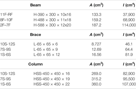
TABLE 1. List of sections of 12-story frame.

First, we investigate the effect of the value of the box constraint parameter $C$ on the accuracy of prediction. For this purpose, we generate another set of 10,000 samples for verification of the results. Table 2 shows the error ratio, the numbers of FNs and FPs in the 1,000 samples, respectively, the number of support vectors (SVs), and the number of SVs with ${\alpha }_i^{\ast }$ value equal to its upper bound $C$, for various values of $C$ using linear and RBF kernels, respectively. Note that the error ratio is the ratio of sum of FN and FP among 1,000 + 1,000 = 2000 samples. The CPU time is also listed. It is seen from Table 2 that the number of SVs with ${\alpha }_i^{\ast }=C$, i.e., the outlier values, is large if $C$ has a large value. By contrast, the error becomes larger as $C$ is increased. Therefore, we select a moderately small value three for $C$ in the following examples. It is seen from the results in Table 2 that RBF kernel has smaller errors than the linear kernel.

TABLE 2

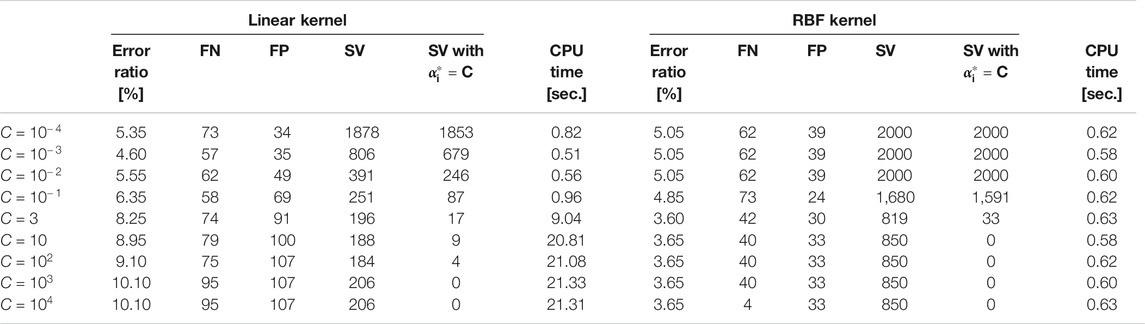
TABLE 2. Error ratio and numbers of FN, FP, SV, and SV with ${\alpha }_i^{\ast }=C$, for various values of $C$ using linear and RBF kernels.

The contribution of a feature, which represents the location and type of a brace, is evaluated using the method described in Identification of Important Features Section. For this purpose, we show that the variation of $c_{ij}$ with respect to i is negligibly small compared with that of $d_{ij}$. For the 12-story 4-span frame, the number of features is $m=5n_f{n}_s=5\times 12\times 4=240$; i.e., $j=\mathrm{1,2},\dots ,240$. The number of SVs as a result of machine learning using RBF kernel is 819, and the samples are rearranged so that the index set for SV is given as $I_{\text{SV}}=\{\mathrm{1,2},\dots ,819\}$. A sample $t=(t_1,t_2,\dots ,t_{48})$, before converting into dummy variables x, is randomly generated as

$\begin{array}{l}t=(\mathrm{2,1,2,1,1,5,1,5,4,5,1,1,2,1,1,3,1,3,1,2,5,1,2,1},\\ \mathrm{2,2,1,1,1,2,2,1,2,1,1,3,2,5,1,1,5,1,1,3,1,4,3,1})\end{array}(16)$

The values of $c_{ij}$ and $d_{ij}$ for all $i\in I_{\text{SV}}$ and $j=1$, for example, are plotted in Figure 4. As seen from these results, the variances of $c_{i1}$ and $d_{i1}$ have the same order. However, the mean, variance, and coefficient of variation (CV) with respect to i for $j=1$ are 0.284, $8.51\times {10}^{-4}$, and 0.10263 for $c_{ij}$, and $1.24\times {10}^{-4}$, $1.92\times {10}^{-4}$, and 111.56 for $d_{ij}$; i.e., $c_{i1}$ has a much smaller CV than $d_{i1}$ because the mean value of $c_{i1}$ is much larger than that of $d_{i1}$. Tables 3A,B show the CVs of $c_{ij}$ and $d_{ij}$, respectively, for the selected features of various samples. Note that the CVs of $d_{ij}$ do not depend on the sample. We can verify from these tables that the CVs of $c_{ij}$ are much smaller than those of $d_{ij}$, which justifies the assumption of constant $c_{ij}$ with respect to i.

FIGURE 4

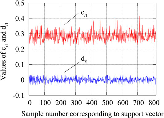
FIGURE 4. Variations of $c_{ij}$ and $d_{ij}$ with respect to i for $j=1$.

TABLE 3

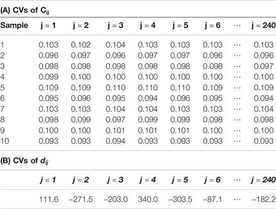
TABLE 3. CVs of $c_{ij}$ with respect to i for various samples.

The features related to the eight largest contributions to be judged as approximate optimal solution are shown in Figures 5A,B for linear and RBF kernels, respectively. Note that the maximum stress exists at the end of a brace in most of the approximate optimal solutions. As seen from the figure, similar features are found in the best solutions by using linear and RBF kernels. Let Li and Ri denote the features with the ith largest contribution in the results using linear and RBF kernels, respectively, computed by Eqs 7, 12. The number of samples containing the specific feature in approximate optimal and non-optimal solutions are denoted by $n_{good}$ and $n_{bad}$, respectively. Contribution of the feature is defined as Ni in Figure 3C in the descending order of $n_{good}-n_{bad}$. Although the orders are different, the same feature considering symmetry of the frame appears in Figures 5A,B,C as L1 = R2 = N1 = N3, L2 = R1, L4 = L7 = R3 = R4 = N2 = N4, L5 = R6, and L8 = R2. This fact explains that the locations and types of the braces are important features for distinguishing the approximate optimal and non-optimal solutions in view of the maximum stress value. Note that the brace locations in the 6th and the 9th stories are important, because the story stiffness change at these stories.

FIGURE 5

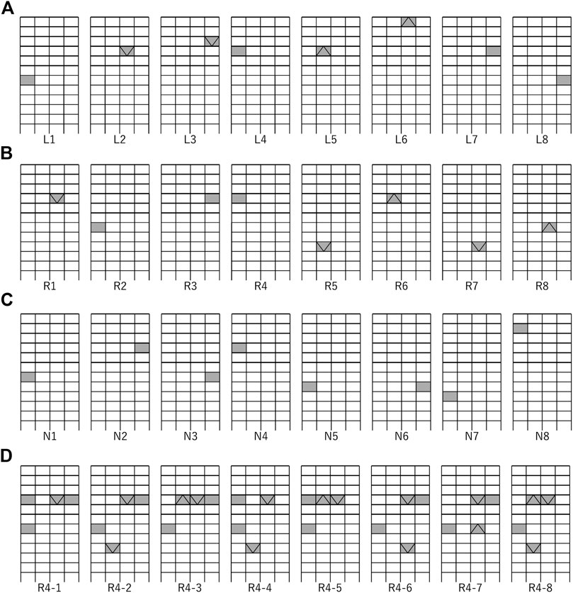
FIGURE 5. Features with the eight largest contributions to approximate optimal solution; (A) linear kernel, (B) RBF kernel, (C) number of samples given as $n_{good}-n_{bad}$, (D) sets of four features using RBF kernel.

The sets of four features corresponding to the eight largest contributions to the approximate optimal solution are plotted in Figure 5D. As seen from the figure, the existence of K- and V-braces in the interior spans of the 4th and 9th stories, as well as non-existence of brace in the outer spans, is important to be classified as an approximate optimal solution.

Application of machine learning results of 12-story frame to 24-story frame.

The machine learning results of the 12-story frame are utilized for optimization of brace locations of a 24-story frame. The story height and span are the same as those of the 12-story frame, which are 3 m and 6 m, respectively. The seismic loads $P_2,P_3,\dots ,P_{23},P_{\text{R}}$ are 10, 14, 19, 23, 27, 32, 36, 41, 46, 50, 55, 60, 65, 71, 76, 82, 88, 95, 102, 111, 121, 135, 156, and 346 (kN). The sections of beams, columns, and braces are listed in Table 4.

TABLE 4

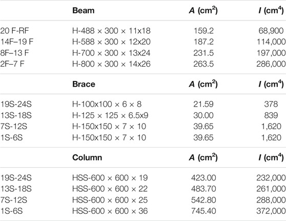
TABLE 4. List of sections of 24-story frame.

The optimization problem Eq. 15 is solved with the parameter $w=1.0$, where $H$ is assumed to be a band matrix with six non-zero components in each row. The value of bias $b$ is 0.473, and the components of the matrix $H$ are shown in Table 5, where the thick gray indicates a large value. No clear rule is observed from the table about the values of the non-zero components in $H$. The CPU time is 161.9 s for generating the learning data, 1.2 s for SVM for the 12-story frame, and 540.2 s for solving the nonlinear programming problem Eq. 15.

TABLE 5

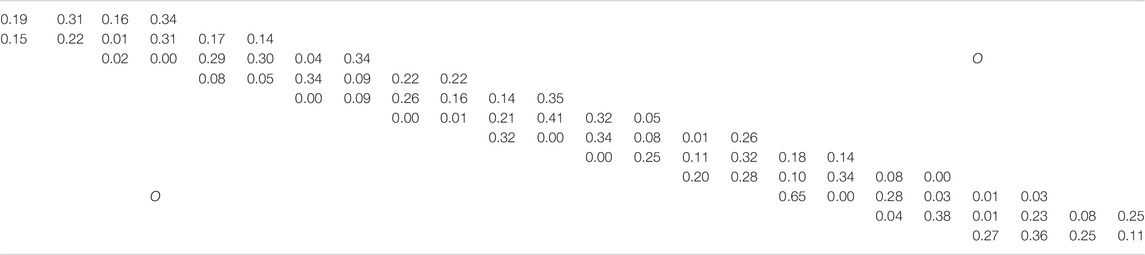
TABLE 5. Components of matrix H.

The errors of application of machine learning results of a 12-story frame to predict the score value of the 24-story frame are shown in Table 6. The RBF kernel is used with the box parameter $C=3$. The results of direct learning of the 24-story frame are also shown. As seen from Table 6, utilizing the results of the 12-story frame leads to about a 20–50% increase of the error from that of the direct learning of the 24-story frame. However, the errors are 2.30% and 1.60%, which are very small, and the numbers of FNs and FPs among 1,000 samples, respectively, are also small for both cases. Table 6 also shows that the absolute value of correlation coefficient R utilizing the results of the 12-story frame is a little smaller than that of the direct learning of the 24-story frame.

TABLE 6

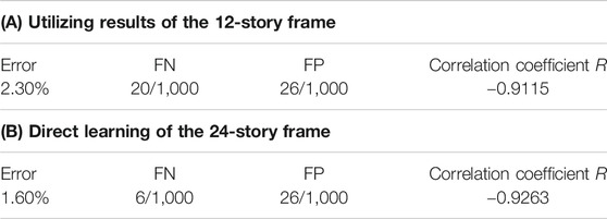
TABLE 6. Machine learning results of 24-story frame.

Figure 6 shows the distribution of scores of approximate optimal and non-optimal solutions of the 24-story frame utilizing the machine learning results of the 12-story frame. It is confirmed that most of the approximate optimal and non-optimal solutions are separated successfully by the score value 0.

FIGURE 6

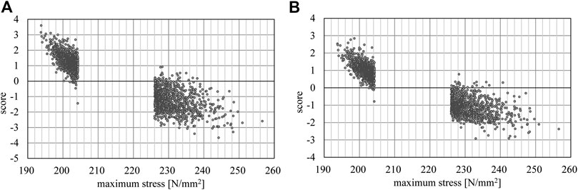
FIGURE 6. Relation between maximum stress of the 24-story frame and the score; (A) linear kernel, (B) RBF kernel.

Since the frame without a brace is symmetric with respect to the center vertical axis, we can assume that the optimal solution is also symmetric. Therefore, the four best and worst symmetric solutions are selected as shown in Figure 7, where the thick line indicates the member with the maximum stress value. We can see from these results that the approximate optimal solutions have braces in the inner span, while many braces are located in the outer span of the non-optimal solutions. Note again that the purpose of this paper is to extract the important features of the approximate optimal solutions. Therefore, we do not intend to optimize the brace locations using the machine learning results only. The learning results will be effectively used in an optimization process as demonstrated in our previous study (Tamura et al., 2018). It is true that the best solutions in Figure 7 are not realistic and large cost will be needed for construction. However, the features in each best solution, not the solution itself, will be utilized for optimization purposes.

FIGURE 7

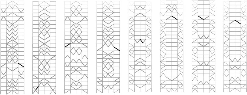
FIGURE 7. Four best and worst solutions in 10,000 samples considering symmetry condition.

In the same manner as the 12-story frame, contribution of the feature is defined in the descending order of the value of $n_{good}-n_{bad}$. The indicator $I_i$ of the ith important feature takes the value one if it is included in the solution and 0 if not. Figure 8 shows the values of $h_i$, which are the cumulative numbers of appearance of features up to the ith important feature, i.e.,

$h_i={\displaystyle \sum _{j=1}^i{I}_j}(17)$

FIGURE 8

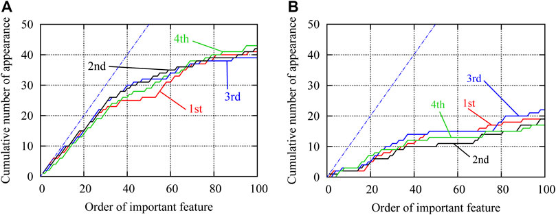
FIGURE 8. Cumulative numbers of appearance of important features existing in the approximate optimal solutions; (A) approximate optimal solutions, (B) non-optimal solutions.

Note that $h_i=i$ is satisfied if all features are included in the solution as indicated in the chain lines in Figures 8A,B. We can see from these figures that more than half of the 50 important features are included in the four best solutions, while only about 20% are included in the four worst solutions. Although differences in these ratios are small, a significant difference exists in the number of solutions that, for example, have all four features.

Number of appearances of features corresponding to the 100 largest contributions to be predicted as approximate optimal solutions are plotted in Figure 9A for the 1,000 approximate optimal solutions classified by utilizing the learning results of the 12-story frame. Note that the large number (around 500–700) of appearances correspond to “no-brace”, and the small numbers (around 200) correspond to the existence of a specific brace that may be doubled if symmetrically located cases are regarded as the same. Figure 9B shows the difference in number of appearances using results of the 12-story frame and direct learning of the 24-story frame, where the latter has larger numbers for all features. It is seen from the figure that the number of appearances for the two cases are almost the same (the maximum difference is four). Therefore, we can conclude that the properties of the approximate optimal solutions of the 24-story frame can be successfully extracted using the machine learning results of the 12-story frame.

FIGURE 9

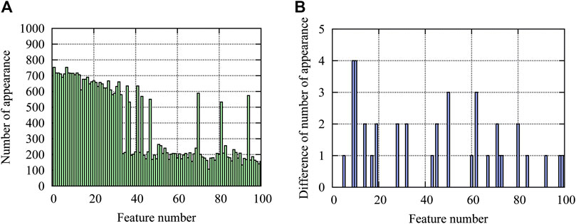
FIGURE 9. Numbers of appearance of features corresponding to the 100 largest contributions to approximate optimal solutions; (A) number of appearance using results of a 12-story frame, (B) difference in numbers of appearance using results of a 12-story frame and direct learning of a 24-story frame.

Conclusion

A method has been presented for extracting important features of the approximate optimal types and locations of braces for a large-scale steel plane frame. A process of seismic retrofitting is assumed and the maximum stress against horizontal seismic loads is minimized under constraints on the maximum interstory drift angle and the number of braces in each story.

The SVM is used for classifying the solutions into approximate optimal and non-optimal solutions. The features representing the types and locations of the braces of a large-scale frame are converted to those of a small-scale frame using a condensation matrix, and its components are identified by minimizing (maximizing the negative value) the correlation between the score and the objective function value. The sum of squares of the score values in the FN and FP solutions are also included in the objective function to determine the appropriate bias value.

A method has also been proposed for identifying the important features of the approximate optimal solutions classified by SVM with RBF kernel functions, where the approximate increase of the score value due to the existence of the specific feature is utilized. Accuracy of this estimation method has been confirmed using the machine learning results of a 12-story frame. The appropriate value of the box parameter has also been investigated.

It has been shown in the numerical examples that the machine learning results of a small-scale (12-story) frame can be successfully used for estimating the properties of the approximate optimal and non-optimal solutions of a large-scale (24-story) frame. A clear difference exists in the cumulative number of appearances of the important features in the approximate optimal solutions and the non-optimal solutions, and each important feature exists in a large number of approximate optimal solutions estimated by utilizing the learning results of the small-scale frame.

The proposed method can be effectively used in the design process of a large-scale braced frame. The results may be utilized for optimization using a heuristic approach in the same manner as our previous study (Tamura et al., 2018). Application to various types of optimization algorithms will be studied in our future research.

Data Availability Statement

The raw data supporting the conclusions of this article will be made available by the authors, without undue reservation.

Author Contributions

KS designed the study, implemented the program, and wrote the initial draft of the manuscript. MO contributed problem formulation and interpretation of data, and assisted preparation of the final manuscript. TK evaluated the results in view of practical design requirements. All authors approved the final manuscript, and agreed to be accountable for the content of the work.

Funding

This study is partly supported by JSPS KAKENHI No. JP18K18898 and JP20H04467.

Conflict of Interest

The authors declare that the research was conducted in the absence of any commercial or financial relationships that could be construed as a potential conflict of interest.

References

Aarts, E., and Korst, J. (1989). Simulated annealing and Boltzmann machines. New York, NY: Wiley.

Google Scholar

Abe, S. (2007). Sparse least squares support vector training in the reduced empirical feature space. Pattern Anal. Appl. 10 (3), 203–214. doi:10.1007/s10044-007-0062-1

CrossRef Full Text | Google Scholar

Abueidda, D. W., Koric, S., and Sobh, N. A. (2020). Topology optimization of 2D structures with nonlinearities using deep learning. Comput. Struct. 237, 106283. doi:10.1016/j.compstruc.2020.106283

CrossRef Full Text | Google Scholar

Adeli, H. (2001). Neural networks in civil engineering: 1989–2000. Comp. Aid. Civil Infrastruct. Eng. 16 (2), 126–142. doi:10.1111/0885-9507.00219

CrossRef Full Text | Google Scholar

Bai, Y., Wang, J., Liu, Y., and Lin, X. (2017). Thin-walled CFST columns for enhancing seismic collapse performance of high-rise steel frames. Appl. Sci. 7 (1), 53–65. doi:10.3390/app7010053

CrossRef Full Text | Google Scholar

Beghini, L. L., Beghini, A., Katz, N., Baker, W. F., and Paulino, G. H. (2014). Connecting architecture and engineering through structural topology optimization. Eng. Struct. 59, 716–726. doi:10.1016/j.engstruct.2013.10.032

CrossRef Full Text | Google Scholar

Cang, R., Yao, H., and Ren, Y. (2019). One-shot generation of near-optimal topology through theory-driven machine learning. Comput. Aided Des. 109, 12–21. doi:10.1016/j.cad.2018.12.008

CrossRef Full Text | Google Scholar

Carmona, L., Sánchez, P., Salvador, J., and Ana, F. (2012). Mathematical methodologies in pattern recognition and machine learning. Berlin, Germany: Springer.

Google Scholar

Cristianini, N., and Shawe-Taylor, J. (2000). An introduction to support vector machines. Cambridge, UK: Cambridge University Press.

CrossRef Full Text | Google Scholar

Dai, H., and Cao, Z. (2017). A wavelet support vector machine-based neural network metamodel for structural reliability assessment. Comput. Aided Civ. Infrastruct. Eng. 32 (4), 344–357. doi:10.1111/mice.12257

CrossRef Full Text | Google Scholar

Do, B., and Ohsaki, M. (2020). Gaussian mixture model for robust design optimization of planar steel frames. Struct. Multidiscip. Optim. 63, 137–160. doi:10.1007/s00158-020-02676-3

CrossRef Full Text | Google Scholar

Glover, F. (1989). Tabu search-Part I. ORSA. J. Comput. 1 (3), 190–206. doi:10.1287/ijoc.1.3.190

CrossRef Full Text | Google Scholar

Hagishita, T., and Ohsaki, M. (2008a). Optimal placement of braces for steel frames with semi-rigid joints by scatter search. Comput. Struct. 86, 1983–1993. doi:10.1016/j.compstruc.2008.05.002

CrossRef Full Text | Google Scholar

Hagishita, T., and Ohsaki, M. (2008b). Topology mining for optimization of framed structures. Jamdsm 2 (3), 417–428. doi:10.1299/jamdsm.2.417

CrossRef Full Text | Google Scholar

Hayashi, K., and Ohsaki, M. (2020b). Reinforcement learning and graph embedding for binary truss topology optimization under stress and displacement constraints. Front. Built Environ., Specialty Section: Computational Methods in Structural Engineering 6Paper No. 59. doi:10.3389/fbuil.2020.00059

CrossRef Full Text | Google Scholar

Hayashi, K., and Ohsaki, M. (2020a). Reinforcement learning for optimum design of a plane frame under static loads. Engineering with Computers. doi:10.1007/s00366-019-00926-7

CrossRef Full Text | Google Scholar

Kallioras, N. A., Kazakis, G., and Lagaros, N. D. (2020). Accelerated topology optimization by means of deep learning. Struct. Multidiscip. Optim. 62, 1185–1212. doi:10.1007/s00158-020-02545-z

CrossRef Full Text | Google Scholar

Kanno, Y., and Guo, X. (2010). A mixed integer programming for robust truss topology optimization with stress constraints. Int. J. Numer. Methods Eng. 83, 1675–1699. doi:10.1002/nme.2871

CrossRef Full Text | Google Scholar

Kennedy, J., and Eberhart, R. C. (1995). “Particle swarm optimization”, in Proceedings of the 1995 IEEE international conference on neural networks. Perth, Australia, 1942–1948.

Google Scholar

Kim, M., Araki, Y., Yamakawa, M., Tagawa, H., and Ikago, K. 2009). Influence of P-delta effect on dynamic response of high-rise moment-resisting steel buildings subject to extreme earthquake ground motions. Nihon Kenchiku Gakkai Kozokei Ronbunshu 74 (644), 1861–1868. doi:10.3130/aijs.74.1861 (in Japanese).

CrossRef Full Text | Google Scholar

Kim, S. H., and Boukouvala, F. (2020). Machine learning-based surrogate modeling for data-driven optimization: a comparison of subset selection for regression techniques. Opt. Lett. 14, 989–1010. doi:10.1007/s11590-019-01428-7

CrossRef Full Text | Google Scholar

Lei, X., Liu, C., Du, Z., Zhang, W., and Guo, X. (2018). Machine learning-driven real-time topology optimization under moving morphable component -based framework, J. Appl. Mech. 86 (1), 1–9. doi:10.1115/1.4041319

CrossRef Full Text | Google Scholar

Li, H.-S., Lü, Z.-Z., and Yue, Z.-F. (2006). Support vector machine for structural reliability analysis. Appl. Math. Mech. 27, 1295–1303. doi:10.1007/s10483-006-1001-z

CrossRef Full Text | Google Scholar

Liu, K., Detwiler, D., and Tovar, A. (2017a). Optimal design of nonlinear multimaterial structures for crashworthiness using cluster analysis. J. Mech. Des. 138, 1–11. 10.1115/1.4037620

Google Scholar

Liu, X., Wu, Y., Wang, B., Ding, J., and Jie, H. (2017b). An adaptive local range sampling method for reliability-based design optimization using support vector machine and Kriging model. Struct. Multidiscip. Optim. 55, 2285–2304. doi:10.1007/s00158-016-1641-9

CrossRef Full Text | Google Scholar

Luo, H., and Paal, S. G. (2019). A locally weighted machine learning model for generalized prediction of drift capacity in seismic vulnerability assessments. Comput. Aided Civ. Infrastruct. Eng. 34, 935–950. doi:10.1111/mice.12456

CrossRef Full Text | Google Scholar

MathWorks, (2016). Matlab user’s manual ver. Natick, MA, USA.

Google Scholar

Nabian, M. A., and Meidani, H. (2018). Deep learning for accelerated seismic reliability analysis of transportation networks. Comput. Aided Civ. Infrastruct. Eng. 33 (6), 443–458. doi:10.1111/mice.12359

CrossRef Full Text | Google Scholar

Nguyen, T., Kashani, A., Ngo, T., and Bordas, S. (2019). Deep neural network with high-order neuron for the prediction of foamed concrete strength. Comput. Aided Civ. Infrastruct. Eng. 34, 316–332. doi:10.1111/mice.12422

CrossRef Full Text | Google Scholar

Ohsaki, M. (2010). Optimization of finite dimensional structures. Cleveland, OH: CRC Press.

Google Scholar

Okazaki, Y., Okazaki, S., Asamoto, S., and Chun, P.-J. (2020). Applicability of machine learning to a crack model in concrete bridges. Comput. Aided Civ. Infrastruct. Eng. 35 (8). 10.1111/mice.12532

CrossRef Full Text | Google Scholar

Panakkat, A., and Adeli, H. (2009). Recurrent neural network for approximate earthquake time and location prediction using multiple seismicity indicators. Comput. Aided Civ. Infrastruct. Eng. 24 (4), 280–292. doi:10.1111/j.1467-8667.2009.00595.x

CrossRef Full Text | Google Scholar

Papadrakakis, M., Lagaros, N. D., and Tsompanakis, Y. (1998). Structural optimization using evolution strategies and neural networks. Comput. Methods Appl. Mech. Eng. 156 (1–4), 309–333. doi:10.1016/s0045-7825(97)00215-6

CrossRef Full Text | Google Scholar

Rahmatalla, S., and Swan, C. C. (2003). Form finding of sparse structures with continuum topology optimization. J. Struct. Eng. 129 (12), 1707–1716. doi:10.1061/(asce)0733-9445(2003)129:12(1707)

CrossRef Full Text | Google Scholar

Saka, M. P., and Geem, Z. W. (2013). Mathematical and metaheuristic applications in design optimization of steel frame structures: an extensive review. Math. Probl. Eng. 2013. 10.1155/2013/271031

CrossRef Full Text | Google Scholar

Senhola, F. V., Giraldo-Londoño, O., Menezes, I. F. M., and Paulino, G. H. (2020). Topology optimization with local stress constraints: a stress aggregation-free approach. Struct. Multidisc. Optim. 62, 1639–1668. doi:10.1007/s00158-020-02573-9

CrossRef Full Text | Google Scholar

Smola, A. J., and Schölkopf, B. (2004). A tutorial on support vector regression. Stat. Comput. 14, 199–222. doi:10.1023/b:stco.0000035301.49549.88

CrossRef Full Text | Google Scholar

Szczepanik, W., Arciszewski, T., and Wnek, J. (1996). Empirical performance comparison of selective and constructive induction. Eng. Appl. Artif. Intell. 9 (6), 627–637. doi:10.1016/s0952-1976(96)00057-7

CrossRef Full Text | Google Scholar

Tamura, T., Ohsaki, M., and Takagi, J. (2018). Machine learning for combinatorial optimization of brace placement of steel frames. Jpn. Archit. Rev. 1 (4), 419–430. doi:10.1002/2475-8876.12059

CrossRef Full Text | Google Scholar

Turan, O., and Philip, S. (2012). Learning-based ship design optimization approach. Comput. Aided Des. 44 (3), 186–195. doi:10.1016/j.cad.2011.06.011

CrossRef Full Text | Google Scholar

U. Stańczyk, and L. C. Jain (2015). Feature selection for data and pattern recognition (Berlin, Germany: Springer).

Google Scholar

Witten, I. H., Frank, E., and Hall, M. A. (2011). Data mining: practical machine learning tools and techniques. Amsterdam, Netherlands: Elsevier.

Google Scholar

Xiong, H., Swamy, M. N., and Ahmad, M. O. (2005). Optimizing the kernel in the empirical feature space. IEEE Trans. Neural Network. 16 (2), 460–474. doi:10.1109/TNN.2004.841784

PubMed Abstract | CrossRef Full Text | Google Scholar

Yonekura, K., and Hattori, H. (2019). Framework for design optimization using deep reinforcement learning. Struct. Multidiscip. Optim. 60, 1709–1713. doi:10.1007/s00158-019-02276-w

CrossRef Full Text | Google Scholar

Yu, Y., Hur, T., Jung, J., and Jang, I. G. (2019). Deep learning for determining a near-optimal topological design without any iteration. Struct. Multidiscip. Optim. 59, 787–799. doi:10.1007/s00158-018-2101-5

CrossRef Full Text | Google Scholar