Monitoring Neutral Axis Position Using Monthly Sample Residuals as Estimated From a Data Mining Model

Introduction

The objective of Structural Health Monitoring (SHM) is to provide a diagnosis of the condition of a structure in at, or near real time. This allows behavioral changes of the structure to be captured and monitored, potentially reducing the cost of maintenance. SHM systems can also be used for early detection of defects that could affect the behavior of a structure, and thereby prevent possible catastrophic failures.

The Neutral Axis (N.A.) of a structural bending element, like a beam, is the intersection of the cross-section in the undeformed geometry with the neutral surface of the bending element, along which no change in length occurs during the deformation of the beam (Shames, 1975). In symmetrical pure bending, the N.A. passes through the area centroid of the cross-section of the beam. When axial loads are applied, the N.A. location is offset from the centroid, while unsymmetrical bending rotates it around the centroid (Boresi and Schmidt, 2003).

Studies regarding the N.A. location on bridge elements (Table 1) have been conducted including lab experiments (Stroh et al., 2010; Papastergiou and Lebet, 2014; Sigurdardottir and Glisic, 2014; Tang and Ren, 2017; Xia et al., 2018; Anastasopoulos et al., 2019), controlled load tests on real structures (Stroh et al., 2010; Gangone et al., 2011; Gangone et al., 2012; Sigurdardottir and Glisic, 2013; Gangone et al., 2014; Sigurdardottir and Glisic, 2014; Xia et al., 2018; Yarnold et al., 2018) and real structures under live loads from traffic (Chakraborty and DeWolf, 2006; Rauert et al., 2011; Oshima and Kado, 2012) or thermal loads (Sigurdardottir and Glisic, 2013). A thorough literature review of these different studies has also been conducted (Sigurdardottir and Glisic, 2015). The study of this parameter extends beyond bridges and has been investigated on other type of structures such as wind turbines (Soman et al., 2018).

TABLE 1

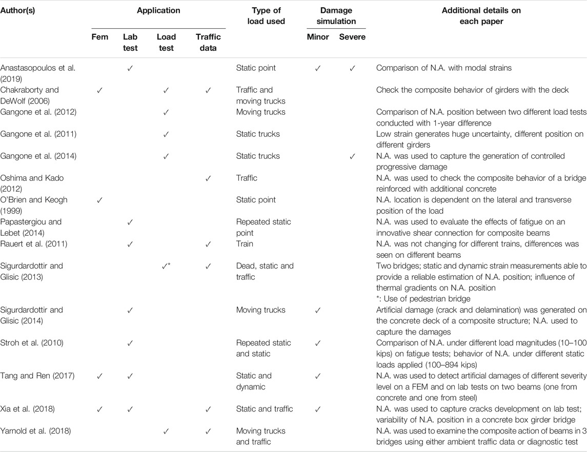
TABLE 1. Characteristics of literature references.

On bridges, for which this research is focused, the location of the N.A. in pure bending has been shown to be independent of temperature (Anastasopoulos et al., 2019). For pure uniaxial bending the N.A. has been shown to be independent of the magnitude of the load (Sigurdardottir and Glisic, 2013); while in wide deck bridges it has been shown that the applied loads affect N.A. location due to biaxial bending effects (O’Brien and Keogh, 1999). In composite structures, N.A. location has been used as a parameter to identify the presence of composite action (Chakraborty and DeWolf, 2006; Yarnold et al., 2018) and also to detect the loss of composite action. For steel girder bridges with composite concrete decks, the N.A. is ideally located in the steel, thereby avoiding the development of tensile cracks in the deck. In several studies, the N.A. location has been successfully used to detect minor (Stroh et al., 2010; Sigurdardottir and Glisic, 2014; Tang and Ren, 2017; Xia et al., 2018; Anastasopoulos et al., 2019) and severe damage (Gangone et al., 2014; Anastasopoulos et al., 2019).

In long-term monitoring of N.A. location, researchers have observed that its position has varied over time, sometimes by a significant amount, and that variation followed a Gaussian distribution around a mean value (Rauert et al., 2011; Oshima and Kado, 2012; Sigurdardottir and Glisic, 2013). Researchers have connected this variability to the uncertainty of the applied loads and the measurement noise (Sigurdardottir and Glisic, 2015). However, monitoring N.A. without defining the applied loads can lead to inaccurate conclusions, if for example, the characteristics of the trucks passing over the bridge changes (trucks passing from different lanes, heavier trucks, etc.). Such variations would offset the mean value of the N.A. location and could incorrectly sound an alarm regarding the condition of the structure.

Research Objectives

The objectives of the research were to 1) identify the factors that affect girder N.A. location when a bridge deck is subjected to traffic loads, 2) use data collected from a SHM system to estimate the effect of these factors, 3) train a model to predict N.A. location, and 4) monitor the differences between the predictions and the actual location as calculated from the measured data. In contrast with what has been done in prior research, the factors affecting N.A. location were considered in the monitoring process. By doing this, the monitoring process becomes more sensitive to truck weight and transverse truck position. Evaluating N.A. location movements with added sensitivity enables structural condition changes to be identified in their early stages of development. The work done herein also represented one of the first known attempts to continuously monitoring the N.A. behavior of bending elements in a long-span (a span length great than 250 ft (76 m)) bridge.

Description of the Cable-Stayed Bridge and the Structural Health Monitoring System

Cable-Stayed Bridge Description

The Charles W. Cullen Bridge, or as it is more commonly known, the Indian River Inlet Bridge (IRIB), is a three-span cable-stayed bridge located in Sussex County, Delaware (Shenton et al., 2017). It carries four lanes of Delaware Route 1 over the Indian River Inlet. Its total length is 1750 ft (533 m), with the main span being 950 ft (290 m) and the two back spans of 400 ft (122 m) each (Figure 1). Four independent pylons with a height of 250 ft (76 m) support the bridge. Bridge construction started in 2009 and it was opened to traffic in 2012. The bridge is composed of precast and cast-in place reinforced concrete elements and is in very good condition (little to no structural deterioration to date).

FIGURE 1

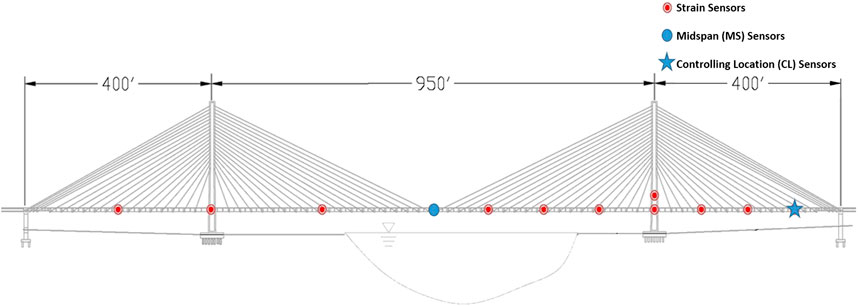
FIGURE 1. Schematic elevation of IRIB, including the longitudinal position of the key sensors.

Structural Health Monitoring System

The Center for Innovative Bridge Engineering at the University of Delaware (UD), in cooperation with the Delaware Department of Transportation (DelDOT), planned and installed a comprehensive SHM system on the bridge during the construction. This system consists of more than 120 individual sensors, distributed throughout the structure, collecting different types of data to evaluate the condition of the bridge (Figure 2).

FIGURE 2

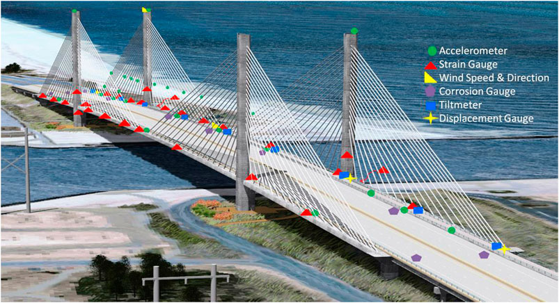
FIGURE 2. Layout of sensors in the SHM system (Shenton et al., 2017).

Strain sensors are installed in different locations along the two longitudinal edge girders of the bridge, in pairs, one located at the top (${\mathrm{\epsilon }}_{\text{TOP}}$) and one at the bottom (${\mathrm{\epsilon }}_{\text{BOT}}$) of the girder (Figure 3). Having two strain measurements on the cross-section, and assuming that the strains developed on the girder vary linearly through the depth, one can calculate the distance y from the bottom of the girder to the N.A. (Figure 3).

$\mathbf{y}=61.5\frac{{\mathbf{\epsilon }}_{\text{BOT}}}{{\mathbf{\epsilon }}_{\text{BOT}}-{\mathbf{\epsilon }}_{\text{TOP}}}+\mathrm{4.5.}(1)$

FIGURE 3

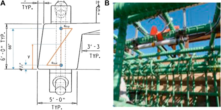
FIGURE 3. Edge girder of IRIB (A) cross-section including strain sensors location, where ε_top and ε_bot refer to the strain measured at the top and the bottom of the section, respectively, and the position of N.A., as distance y from the bottom of the girder, assuming linear strain development (B) photograph from the installation of sensor during construction.

This research focused on the N.A. position, of the west girder, in the middle of the Main Span (MS) and at the location that controls the load rating of the bridge on the backspan, the Controlling Location (CL) (Figure 1). These locations were selected because they experience the highest live-load strains.

Diagnostic Load Tests Conducted in the IRIB

Non-destructive diagnostic load tests of the IRIB have been conducted periodically to evaluate its condition under controlled conditions and for known truck loads (Al-Khateeb et al., 2019; Chajes et al., 2020). The first load test was conducted after the completion of construction (April 2012), followed by tests after 6 months, 1 year, 2 years and repeated every 2 years after that. The tests are conducted at night to reduce the thermal and solar effects and to reduce impacts on the local traffic. Different truck configurations are used including single-, four-, and six-truck passes. Normal traffic is restricted during the load passes. A 10–15 s window is captured before each pass, with the bridge free of traffic, which is used to zero the initial measurements.

The N.A. location was calculated for all of the load passes at the two locations (MS and CL) on the bridge. Strain-time histories were post-processed using a 0.32 s moving average to eliminate some of the inherent noise. The 0.32 s average amounts to a 5-point average for the 12.5 Hz sample rate used by the SHM system to capture live load traffic effects. It was found to eliminate most of the low-level noise and vibration of the live load strains and still yield an accurate measurement of the peak stain. To be consistent, the same averaging window was used for the load test results. Due to remaining noise, and the imperfection in replicating the passes (Aloupis et al., 2019), variability still exists when comparing similar passes. To further minimize the effect of this variability on the calculation of the N.A., the location was calculated only when the magnitudes of both the top and bottom strain measurements were greater than 10 με, as small strains can yield large errors in the calculation of N.A., as evident by inspection of Eq. 1. Furthermore, the limit of 10 με was identified as a general agreement between the different studies on N.A. (Sigurdardottir and Glisic 2015).

Static Loads

The examination of the data started with the truck “pass” providing the best conditions for a consistent estimate of the N.A. location: a static load resulting from six side-by-side trucks stopped at the middle of the main span. Figure 4A shows a time history plot of the N.A. location as the six trucks cross the bridge and stop at mid-span. One can see that under these ideal conditions (a large static load) the N.A. location at midspan is quite stable when the vehicle is stationary, varying only slightly around a mean value. Another interesting feature of the behavior is the drop of the N.A. at the beginning, which represents the time that the trucks are approaching mid-span and then stop.

FIGURE 4

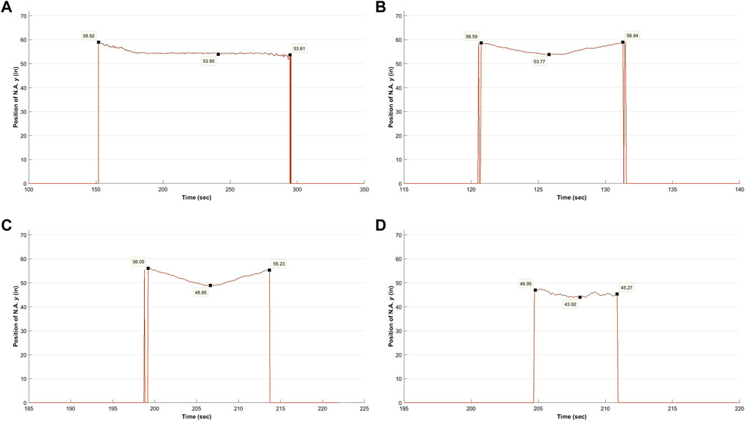
FIGURE 4. Time histories of N.A. position y (as measured from the bottom of the girder) in the west girder during load test 6 (A) at midspan (MS) under the static load of six trucks, (B) at midspan (MS) during the six-truck pass, (C) at controlling location (CL) during the six truck pass, and (D) at controlling location (CL) during the single-truck pass. N.A. is only printed for times that both top and bottom sensor exceeded 10 με.

Moving (Pseudo-static) Loads

For the moving passes, trucks crossed the bridge at a crawl speed of approximately 5 mph. These applied loads are pseudo-static. Sample time histories of the N.A. location when both the top and bottom strain sensors are greater than 10 με are presented in Figures 4B–D. From these time histories it can be observed that:

• The N.A. location varies with the longitudinal position of the trucks. It makes a curve in all of the time histories in Figure 4. The N.A. moves down (lower) in the cross-section until it reaches a minimum value and then it moves back up. This behavior shows a correlation between N.A. location and the longitudinal position of the load. The N.A. moves higher (upwards) in the cross-section the further the load is from the sensor location.

• The N.A. location in the cross-section varies along the length of the girder. The different axial loads developed in the girders, due to the cable forces, makes every cross-section of the bridge unique. For that reason, the N.A. location should be estimated for each girder sensor location separately. By comparing Figures 4B,C, one can see that the difference in the minimum N.A. location between the middle of the main span (MS, 53.77 in) and the controlling location (CL, 48.85 in) in the back span could be up to 5 in (127 mm), under the same applied loads.

• The N.A. position varies with the magnitude of the load. By comparing the single-truck passes with the six-truck passes, it was observed that at the controlling location the N.A. is 5 in (127 mm) higher in the six-truck passes. The correlation between the magnitudes of the applied load with N.A. location was observed in all the examined locations of the bridge (middle of main span and control location for both girders).

• The N.A. location cannot be estimated for all truck passes. For the single-truck passes, only the passes in the lanes closest to the girder of interest cause strains greater than 10 με both in the top and the bottom of the girder. For the west side both for the MS and CL locations, the passes in the two lanes and the shoulder closest to the west girder cause strains higher than the limit, while for the east side the presence of a pedestrian lane offsets the traffic lanes and therefore the truck passes in which N.A. locations are considered are only the shoulder and the slow lane.

Having seen the variability of N.A. over the different passes and the presence of minimums, it was decided to compare the peak values of the different passes over the load tests at the controlling location (Figure 5). Some of the previous observations were confirmed from this graph, however there are also several new observations:

• The results agree with the well-understood correlation between the N.A. location and the magnitude of the applied load. Basic concrete beam behavior in bending result in an upward movement of the neutral axis with increased bending moment. What is notable here is that for a bending element with significant dead loads, the effects on the neutral axis poisiton due to live loads are so significant (and therefore useful in detecting structural condition changes). In the six-truck passes, the N.A. is noticeably higher than it is for the four truck passes, and the six- and four-truck passes are both significantly higher than any of single truck pass.

• As the magnitude of the applied load increases, the consistency of the measurements increases as well. The large strains developed both in the top and the bottom of the girder, due to heavier loads, reduce the impact of the measurement noise on the N.A. calculation.

• One can also see that the lateral position of the load (the traffic lane the trucks pass) affects the N.A. location. This becomes clear when comparing single truck passes in the shoulder with those in the fast lane: the N.A. moves downward, when the load is approaching the girder of interest. That change could be a result of the effective width (getting far from the edge girder, the strain is distributed in larger area of the deck), from biaxial bending (N.A. is not going up and down, but it rotates), or from increase of the axial forces (cable loads) applied on the girders.

FIGURE 5

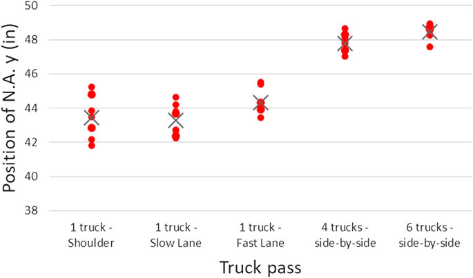
FIGURE 5. N.A. minimum values in the west edge girder at controlling location (CL) over the different passes of the load tests (single truck passes in the southbound lanes). X sign represents the average position of N.A. y for each different pass.

Live Load Traffic Data Collected From the IRIB

The data from the controlled load tests is good for drawing preliminary conclusions about the behavior of the N.A. and how it changes when the loads are changing. However, more refinement is needed to use the N.A. location to accurately monitor the behavior of the bridge. The variability of the N.A. position for the same truck passes over different tests shows the effect of the noise and the difficulty it would present in using N.A. location measured from a load test as an indication of changes in the bridge. Greater amounts of data would provide more reliable feedback on bridge condition, since statistical parameters could be used to eliminate noise effects. This larger amount of data can be gathered from the ambient traffic data. The continuous data collected by the SHM system were used to capture trucks crossing the bridge and monitor the behavior of the N.A. based on indirect estimations of the vehicle weight and lateral position on the bridge.

Data is collected continuously, 24/7, at a rate of 12.5 Hz, by the SHM system. This “high frequency” data is used to capture trucks and other heavy vehicles as they cross the bridge. Unfortunately, the weight and lane in which these vehicles travel are unknowns (there is no weigh-in-motion system on, or immediately adjacent to, the bridge). As seen from the load tests, weight and lateral position of a vehicle affect the location of the N.A., so if these are not considered when monitoring N.A., changes in their distribution could change the distribution of N.A. position and falsely trigger alerts. Therefore, a first objective was to find an indirect way to estimate the weight and lateral position of a vehicle from the live load traffic data. The weight is estimated by the sum of the strains measured on the bottom of the east and west edge girders at the same longitudinal position on the bridge, since these strains are well correlated.

${\mathbf{W}}_{\text{est}}\propto {\mathbf{\varepsilon }}_{\text{BOT}}^{\mathbf{W}}+{\mathbf{\epsilon }}_{\text{BOT}}^{\mathbf{E}}\mathrm{,}(2)$

where ${\mathbf{W}}_{\text{est}}$ represents the weight proportional strain, and ${\mathbf{\epsilon }}_{\text{BOT}}^{\mathbf{W}}$ and ${\mathbf{\epsilon }}_{\text{BOT}}^{\mathbf{E}}$ are the strains on the bottom of the west and east girders, respectively. The lateral position is estimated using the ratio of the strain measured on the bottom of the girder of interest divided by the sum of east and west bottom strains.

$\mathbf{P}=\frac{{\mathbf{\epsilon }}_{\text{BOT}}^{\mathbf{i}}}{{\mathbf{\epsilon }}_{\text{BOT}}^{\mathbf{W}}+{\mathbf{\epsilon }}_{\text{BOT}}^{\mathbf{E}}};\mathbf{i}=\mathbf{W}\text{or}\mathbf{E},(3)$

where $0\le \mathbf{P}\le 1$. This is a measure of the transverse load distribution to the two edge girders; the closer P is to one, the closer the vehicle is to the girder or interest. Finally, to exclude the effect of the longitudinal position of the load, only the point in time when the largest strain in the bottom sensor occurs is used in the calculation (this point was usually also the point that the top sensor was developing the largest strain).

Data collected for the 22 months between March 2015 and December 2016 were used in the analysis. For this period, a 2-min moving average was first used to calculate the strain due to slowly changing loads, such as thermal effects. This moving average was subtracted from the full measurements to yield the strains developed due to vehicles and any other live loads. Since the focus of the N.A calculation was on traffic loads, it was necessary to understand what variability in the measurement could be caused by system noise and also by dynamic loads that couldn’t be measured, such as wind loads. Wind loads for a long span bridge like IRIB can have a large impact even for moderate winds. To reduce the effect of these two factors (noise and unknown dynamic loads), the live load data were smoothed, again using a 0.32 s moving average, as was used in the load tests. With the data free of thermal effects and slightly smoothed, a truck pass event was assumed each time both the top and the bottom sensors on the girder of interest exceeded the 10 με limit. The measurements were collected, together with the strain measurement developed on the bottom of the opposite edge girder, with no strain limitation. Using these three values, the N.A. location and the values related to the truck magnitude and the lateral position were calculated for the west girder. Based on the load tests, where the trucks were weighted before used, the development of 10 με in both sensors (top and bottom) of the girder of interest, needs a minimum vehicle weight of 36.5 kips.

Characteristics of the Collected Traffic Data

Over the 22 months there were 17,418 events (passage of a heavy load as prescribed by the 10 με threshold) captured based on the measured strains at the controlling location (CL) of the west girder. The number of events is equivalent to about 26 per day, which is reasonable since the bridge is in a remote beach community and not a heavily traveled truck corridor. The three strain measurements that were used to calculate the N.A. position at the controlling location, were: West girder top sensor (S_W21), West girder bottom sensor (S_W22), and East girder bottom sensor (S_E22).

The distributions and quantiles for the N.A. location, magnitude of the load, and lateral position are shown in Figure 6, as computed and plotted using JMP Pro (SAS Institute). The distribution of the N.A. location ranges from 39.7 to 52.8 in (Figure 6A). The summations of the strains at the bottom of the two girders, or the indirect estimation of the magnitude of the load, starts at 14.41 με and reaches a high of 97.12 με, with 80% of them falling between 31 and 49 με (Figure 6B). Finally, from the distribution for the lateral position, it can be seen that the majority of the events that were captured resulted from trucks in the lanes close to the west girder, i.e., positions closer to 1.0 than 0.0 (Figure 6C). This is explained from the criteria set for an event to be captured; both top and bottom sensors in the girder of interest must exceed 10 με. In order to capture a truck passing in a lane far from the west girder it must be very heavy. Some trucks that manage to do that are represented in the outliers in the bottom of the lateral position distribution (Figure 6C).

FIGURE 6

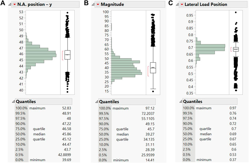
FIGURE 6. For the controlling location (CL) of west girder the distribution of (A) N.A. position (in), (B) magnitude of the trucks weight (με), and (C) lateral position of the truck traffic (unitless).

The data collected from the traffic loads confirmed the findings of the diagnostic load test. As was seen from the load tests, as the magnitude of the applied load increases the N.A. location moves higher in the cross-section, which can be seen in the traffic data (Figure 7A). In the figure, blue dots indicate trucks with a lateral position greater than 0.5 (closer to the west girder), while the red dots represent trucks with a lateral position smaller than 0.5 (closer to the east girder). Trucks developing a combined bottom strain greater than 70 με were captured even when they were passing on the opposite side of the bridge. Trucks being far from the west girder produce strains that move the N.A. higher in the cross-section, just as observed in the load tests. That correlation of the N.A. position with the lateral position of the applied load was seen in all the traffic data collected (Figure 7B).

FIGURE 7

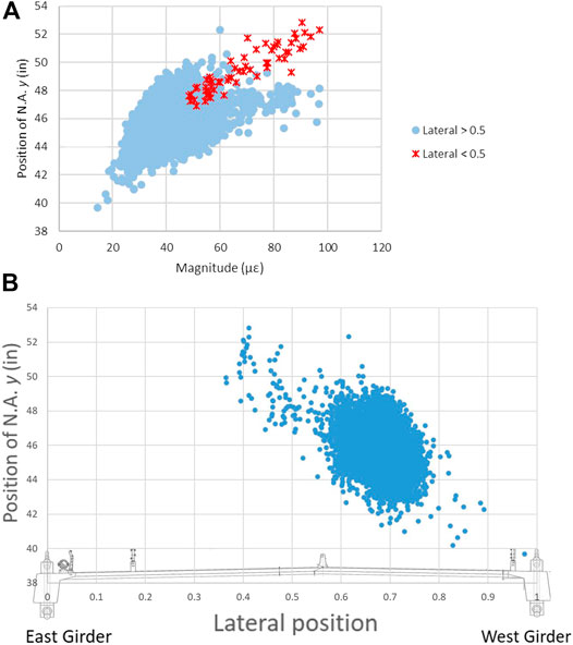
FIGURE 7. West girder N.A. position at the controlling location (CL) vs (A) Magnitude of the truck weight (summation of the strains measured on the two bottom sensors) grouped based on the proximity to the girder, and (B) Lateral position (strain measured on the bottom of the girder of interest over the summation of the strains measured on the two bottom sensors) of the truck traffic.

Training of Data Mining Model to Predict N.A. Position

Knowing that N.A. changes based on the magnitude and the position of the applied loads, a way to estimate the N.A. location based on these two parameters is proposed. If successful, changes in bridge condition could be indicated by the difference between the measured and predicted N.A. location based on the characteristics of the loads, i.e.,

${\mathbf{r}}_{\mathbf{i}}={\left({\mathbf{y}}_{\mathbf{m}}-{\mathbf{y}}_{\mathbf{p}}\right)}_{\mathbf{i}},(4)$

where ${\mathbf{y}}_{\mathbf{m}}$ and ${\mathbf{y}}_{\mathbf{p}}$ are the measured and predicted N.A. location for data sample i, and ${\mathbf{r}}_{\mathbf{i}}$ is the ith residual. A positive residual would mean that the measured N.A. position is higher than the predicted, which means that N.A. has moved higher in the cross-section, while a negative residual would mean that it has moved lower in the cross-section. Movements of the N.A. can be related to different types of problems: the development of a crack at the bottom of a girder would move the N.A. higher. While not an issue for the IRIB, the loss of composite action of a concrete-steel composite cross-section would move the N.A. lower in the cross-section. For that reason, knowing the direction that the N.A. is moving is important.

To do this, a data mining model was trained using the data collected from the first 3 months (March 2015 to May 2015) to predict the N.A. location based on the magnitude (${\mathbf{W}}_{\text{est}}$ ) and the lateral position (P) of the load as described earlier (Figure 8). The data mining model was trained using Weka, a program developed at the University of Waikato in New Zealand and the technique selected was the M5P tree (Wang and Witten, 1996), which combines a conventional decision tree with the possibility of linear regression functions at the nodes. Even though the data were not free of noise, the large amount of data eliminated the noise effect on the training process, producing a free of noise model. The trained model was then fed with the remaining 19 months of data to validate it. For each point, the value predicted by the model was compared with the actual value as calculated using the top and bottom strain measurements.

FIGURE 8

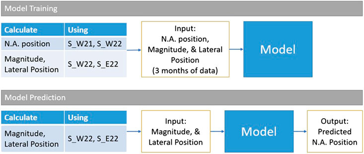
FIGURE 8. Data mining model trained to predict N.A. position based on the estimations of the Magnitude and the Lateral Position of the traffic load.

Four different models were used to predict N.A. location: 1) a model based on the average of the 3 months of training data, 2) a model based on the strain developed at the bottom of the west girder, 3) a model based on the magnitude of the applied load (${\mathbf{W}}_{\text{est}}$), and 4) a model based on both magnitude (${\mathbf{W}}_{\text{est}}$) and lateral position (P) of the applied load. The distributions of the residuals for the four models are shown in Figure 9.

FIGURE 9

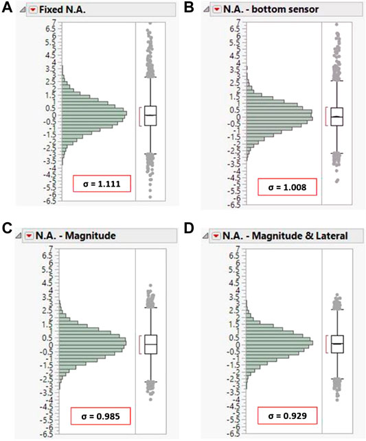
FIGURE 9. Distribution of residuals from the four different models: (A) fixed N.A., (B) N.A. estimated based on bottom sensor measurement, (C) N.A. estimated based on magnitude of the applied load, and (D) N.A. estimated based on magnitude and lateral position of applied load.

As the data mining model improves, the standard deviation of the residuals decreases, leading to sharper distribution curves. One can see that the model with both magnitude and lateral position has the smallest standard deviation and a slightly sharper distribution of residuals. The improvement of the model is even clearer from the box-and-whisker plots, where quantile values are closer to zero and the outliers have been reduced both in number and magnitude. Of special interest is the improvement of the maximum value of residuals captured by each of the models. In the approach, where the N.A. position should be considered constant (see Figure 9A), the maximum residual captured was 7 in. compared to the 3.5 in. seen in the proposed method. A smaller standard deviation means that the control limits are smaller, and the system should be more sensitive to capturing changes. The outliers are less because their majority on the other models occurs due to loads that have different characteristics than the average loads, such as very heavy trucks or different lane patterns. The reduced number of outliers means that the system will potentially have fewer false alarms if the N.A. is monitored and used as a trigger.

Effect of Noise on Accuracy of Measurements

The effect of low-level vibrations and system noise on the predicted N.A. location have been investigated. To do that, data were collected between 12:00 and 4:00 am for 50 randomly selected nights throughout the year. Night data were used due to the low traffic volume at night on the bridge. The data were processed to eliminate the thermal effects and smoothed using the same procedure used for the traffic data. Any data following a pattern that indicated a truck passing were removed. This way, the data only reflected the effect of system noise and undefined loads such as wind. The standard deviation of the measured data from the three key sensors was 0.72 με for S_W21, 0.75 με for S_W22, and 0.69 με for S_E22.

Knowing the distribution of the variability for each of the sensors, a Monte Carlo (MC) simulation was conducted to generate different load scenarios with simulated noise to see the effect of the noise on the distribution of the residuals. Details of the Monte Carlo (MC) simulations are presented in the Supplementary Material.

By comparing the residuals from the MC simulation with the residuals of the actual traffic data collected on the bridge (Figure 10), one can see a very good correlation, which means that the residuals could be explained for the most part by the expected variability in the data. The good correlation is primarily shown in the quantile tables, where the differences are, most of the time, less than 0.1 in. Even the standard deviations of the residuals are very close: σ = 0.93 for the actual traffic and σ = 0.88 for the MC residuals. Overall, the simulation shows that the residuals could be explained by the uncertainty in the strain measurements, while the small changes are probably due to imperfect data that was used to train the model. Using more data for training should reduce these changes. Another reason for these differences could be the variability on the longitudinal position of the load (the variability could have offset the peak point of the strains).

FIGURE 10

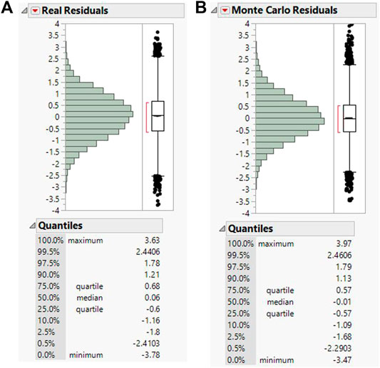
FIGURE 10. Comparison of (A) actual N.A. residuals with (B) the N.A. residuals from MC simulation for the west girder at the controlling location (CL).

Change in Distribution of Truck Weights

The importance of taking into account parameters affecting N.A. position can be seen in the results of another Monte Carlo simulation. Here, a change in the distribution of truck weighs has been investigated. To study this, the distribution of the loads captured from the real data were used, but the mean value was increased by 50%. By generating random loads from the revised distribution and feeding them into the data mining model, the N.A. position was predicted. Comparing Figures 11A,B, one can see how the distribution of the N.A. location would be affected by the change in the characteristics of the loads. The increased load caused a significant change in the mean value of the N.A. of almost 0.6 in and, most importantly, generated values that are higher in the cross-section than had been seen before. If the N.A. was monitored without considering the truck weights, this change could have been misconstrued as a change in behavior of the structure, such as damage and triggered a false alarm. However, when the load characteristics (magnitude and lateral position) are taken into account, the distribution of the residuals (Figures 11C,D) remains around zero, with the distribution getting sharper in Figure 11D, because the effect of noise is smaller for the larger loads. Figure 11 demonstrates the advantage of this method by being independent of the applied loads. This method will trigger an alarm when actual behavioral changes occur and not due to change of the traffic patterns, such as heavier trucks.

FIGURE 11

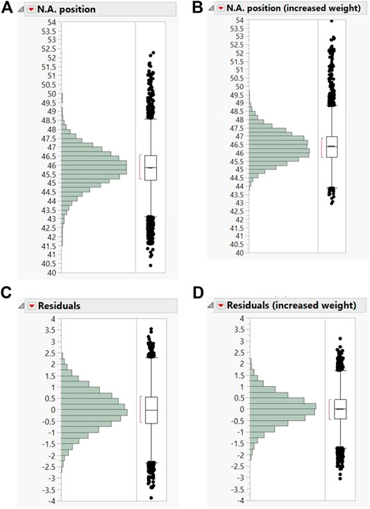
FIGURE 11. (A) N.A. position for regular trucks weights vs (B) N.A. position for increased truck weights, (C) Residuals from method for regular truck weights vs (D) Residuals from method for increased truck weights.

Monitoring the Distribution of Residuals on a Monthly Basis

The use of data mining techniques to find the correlations of N.A. location with magnitude and lateral position of the load reduced the variability of the residuals of the N.A. However, noise is still a problem that can hide small changes. MC simulation showed that a residual of even four in. could be explained by noise, making it difficult to capture small changes. To attempt to minimize the noise effects, changes in the distribution of N.A. residuals on a monthly basis was selected to be monitored instead of individual values.

Monthly Distributions

The monthly sample size of 800 events is large enough to have consistent distributions and support reliable conclusions. While this would mean a possible delay in a month of detecting a change in behavior, this is far more desirable when compared to a possible 2-years delay that could occur with the regularly scheduled inspections.

Figure 12 presents an example of 1) the histogram of the monthly distribution (June 2015) and its fit to the normal distribution, and 2) the cumulative distribution function. The seven colored data points represent the points of interest that will be monitored on a monthly basis for capturing changes. These points show which proportion of the monthly data that have residuals smaller than −3, −2, −1, 0, 1, 2, and 3 in (Figure 12B). From these 19 months (Figure 12C) it can be observed that, each month:

• 100% of data are between −3 and 3. Observations captured in some months are much lower than 0.5% and, for that reason, they are not shown on the graph.

• The negative values represent from 42 to 56% of the residuals, varying around 50%.

• Residuals less than −2 in are 1–3%, exactly like residuals more than 2 in (in the cumulative graph, that’s represented by values from 97 to 99% for values less than 2 in).

• 9–20% is the range of the cumulative frequencies for residuals smaller than −1 in and 81–88% for smaller than 1 in.

FIGURE 12

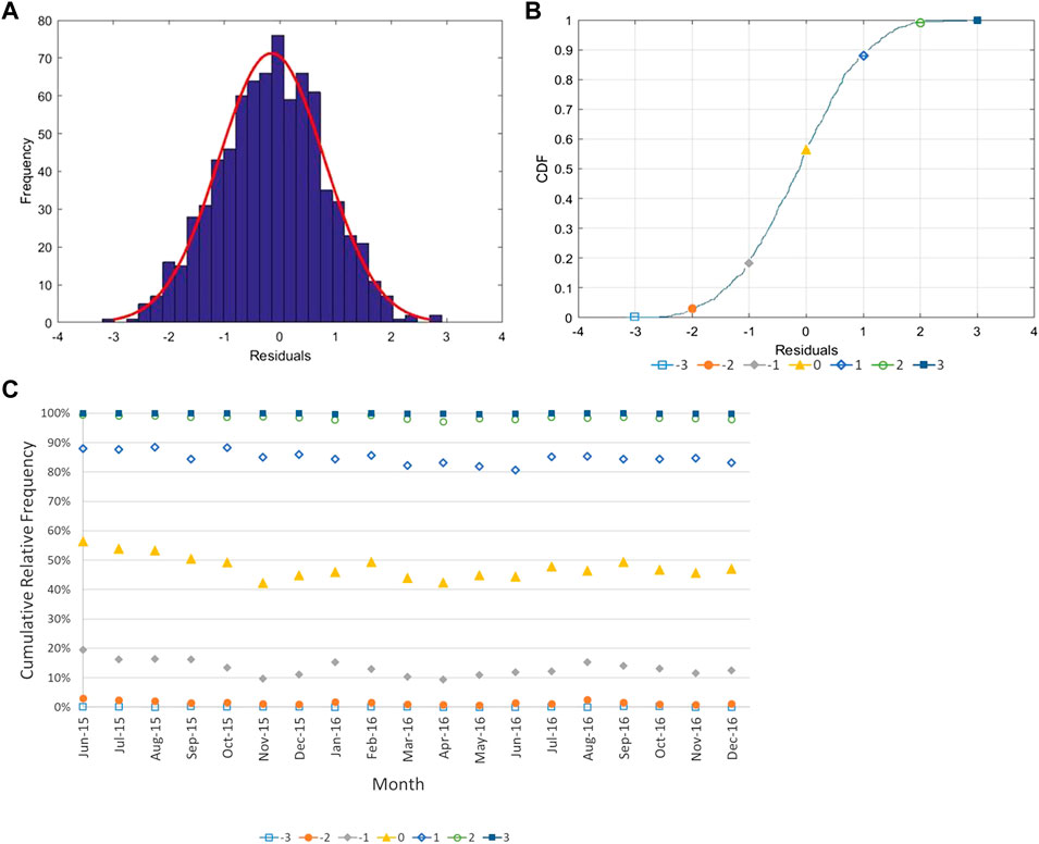
FIGURE 12. (A) Frequency distribution and (B) Cumulative distribution function of residuals for June 2015 at the controlling location (CL) of west girder (C) Key points of cumulative distribution function for monthly residuals at controlling location (CL) of west girder.

As expected, the distributions are shown to be consistent over these 19 months in Figure 12C. This consistency is even clearer in the next section where small changes are simulated in the N.A. position.

Sensitivity of Distributions

MC simulations were conducted to evaluate the sensitivity of the distributions to changes of N.A. behavior. The N.A. that was expected based on the specific loads was moved using a fixed value (different value for each scenario) and based on the new “changed” position S_W21 was calculated. Three different scenarios were conducted with results shown in Table 2: 1) N.A. offset upwards by 0.5 in, 2) N.A. offset downwards by 0.5 in and 3) N.A. offset downwards by 0.25 in.

TABLE 2

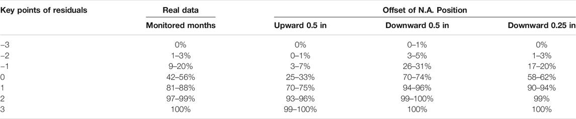
TABLE 2. Range of cumulative distribution function for key points of residuals for the real data and simulated behavioral changes of N.A. position.

One can see the range that each of the cumulative frequencies took during the three scenarios and compare it with the actual values measured by the system. It can be seen that for a 0.5 in. offset of N.A., in both directions, the distribution of residuals changes significantly, and it can be captured from one month of data. On the other hand, for a 0.25 in. change, a second month might be needed to clarify the overlap of some of the frequency windows. However, if data of multiple months are on the edges of the range window, this would be an indicator of behavioral change.

Conclusion

Using the location of the N.A. has shown great potential for identifying changes in the condition of a structure. For that reason, multiple researchers have investigated using it as a parameter to be monitored. However, it has been found that the location of the N.A is affected by various parameters. Both controlled load tests and response from ambient traffic loads have been used to show that N.A. location depends on the magnitude of the vehicle loads and lateral position of the applied load (travel lane). This effect was significantly higher than what one would expect from a dead load driven structure, like the IRIB. Prior studies have shown that monitoring N.A. distribution can be used to identify composite behavior of a cross section, but not necessarily in a general damage detection process, since changes in the characteristics of the applied load (truck patterns) can change the distribution of N.A. location and may therefore not be a good indicator of possible damage.

A new methodology that addresses these shortcomings has been presented. The method uses N.A. locations computed based on live load girder stains. From the strains, an indirect estimate of the vehicle weight and transverse position, properties that affect the N.A. position, can be determined. Using these estimations, a data mining model was trained to predict N.A. locations, which can then be compared to the values computed using measured top and bottom strains. By doing this it was shown that the residuals between the predictions and the actual values can be separated from the residuals caused by changes due to the characteristics of the traffic loads. Using distributions of the residuals, a method for increasing significantly the sensitivity of N.A. location changes was demonstrated, allowing one to capture changes as small as 0.25 in (0.635 cm), compared to the 7 in (17.78 cm) variability shown when using the N.A. location itself. With the added sensitivity, early stages of damage development can be captured. The amount of data needed for reliable detection depends on the frequency and weight of trucks crossing the bridge. The amount of data should be small enough to inform the owner in a timely manner about changes in behavior, but large enough to be reliable. In the bridge studies conducted herein on the IRIB (which has low volumes of truck traffic), one month of data were found to be sufficient.

Data Availability Statement

The raw data supporting the conclusion of this article will be made available by the authors, without undue reservation.

Author Contributions

CA, HS, and MC contributed to the conception and design of the study; HS was in charge of developing the SHM system and oversaw all of the load tests; CA performed the data analysis; CA, HS, and MC wrote portions of the first draft of the manuscript. All authors contributed to manuscript revision and read and approved the submitted version.

Funding

The project was supported by funds from both the Delaware Department of Transportation and the Federal Highway Administration under grants BRDG422145–09001448, BRDG422158–TASK 30A–1717, BRDG422161–TASK 30B–1717, and BRDG422162–TASK 30C–1717.

Conflict of Interest

The authors declare that the research was conducted in the absence of any commercial or financial relationships that could be construed as a potential conflict of interest.

Acknowledgments

The authors would also like to acknowledge a number of individuals, agencies, and firms for their support and role in developing and implementing the structural health monitoring system for the Indian River Inlet Bridge and for their assistance in conducting the controlled load test. These include the Delaware Department of Transportation for the financial support to develop and implement the structural monitoring system, and for help during the load tests (Doug Robb, Craig Stevens, Marx Possible, David Gray, Alastair Probert, Jason Arndt, Craig Kursinski, Raymond Eskaros, and the crew from the southern district); the Federal Highway Administration for the financial support to develop and implement the structural monitoring system; Cleveland Electric Labs/Chandler Monitoring Systems (Jim Zammataro, Keith Chandler, Jennifer Chandler, and Abee Zeleke); and University of Delaware students for their help during the load tests and other activities (Hadi Al-Khateeb, Pablo Marquez, Nakul Ramana, Jack Cardinal, and Patrick Carson).

Supplementary Material

The Supplementary Material for this article can be found online at: https://www.frontiersin.org/articles/10.3389/fbuil.2021.625754/full#supplementary-material.

References

Al-Khateeb, H. T., Shenton, H. W., Chajes, M. J., and Aloupis, C. (2019). Structural health monitoring of a cable-stayed bridge using regularly conducted diagnostic load tests. Front. Built Environ. 5, 41. doi:10.3389/fbuil.2019.00041

CrossRef Full Text | Google Scholar

Aloupis, C., Chajes, M. J., and Shenton, H. W. (2019). “Quantification of uncertainties in diagnostic load test data,” in Proceedings of the Bridge Engineering Institute Conference, Rome, Italy, July, 2019.

Google Scholar

Anastasopoulos, D., De Roeck, G., and Reynders, E. P. B. (2019). Influence of damage versus temperature on modal strains and neutral axis positions of beam-like structures. Mech. Syst. Signal Process. 134, 106311. doi:10.1016/j.ymssp.2019.106311

CrossRef Full Text | Google Scholar

Boresi, A. P., and Schmidt, R. J. (2003). Advanced mechanics of materials. 6th Edn. New York, NY: John Wiley and Sons.

Chajes, M. J., Shenton, H. W., Al-Khateeb, H. T., and Aloupis, C. (2020). Establishing baseline performance of a segmental-concrete cable-stayed bridge. Naples, FL: ACI Symposium Publication, 340.

Chakraborty, S., and DeWolf, J. T. (2006). Development and implementation of a continuous strain monitoring system on a multi-girder composite steel bridge. J. Bridge Eng. 11, 753–762. doi:10.1061/(asce)1084-0702(2006)11:6(753)

CrossRef Full Text | Google Scholar

Gangone, M. V., Whelan, M. J., Janoyan, K. D., and Minnetyan, L. (2014). Development of performance assessment tools for a highway bridge resulting from controlled progressive monitoring. Struct. Infrastruct. Eng. 10, 551–567. doi:10.1080/15732479.2012.757329

CrossRef Full Text | Google Scholar

Gangone, M. V., Whelan, M. J., Janoyan, K. D., and Minnetyan, L. (2012). Experimental characterization and diagnostics of the early‐age behavior of a semi‐integral abutment FRP deck bridge. Sens. Rev. 32, 296–309. doi:10.1108/02602281211257533

CrossRef Full Text | Google Scholar

Gangone, M. V., Whelan, M. J., and Janoyan, K. D. (2011). Wireless monitoring of a multispan bridge superstructure for diagnostic load testing and system identification. Comp-Aided Civil and Infrastruct Engineering. 26, 560–579. doi:10.1111/j.1467-8667.2010.00711.x

CrossRef Full Text | Google Scholar

Oshima, Y., and Kado, M. (2012). “Long-term monitoring of composite girders using optical fiber sensor,” in Proceedings of the 6th International Conference on Bridge Maintenance. Safety and Management, Barcelona, Spain, July, 2012.

Google Scholar

O’Brien, E. J., and Keogh, D. L. (1999). A discussion on neutral axis location in bridge deck cantilevers. Comput. Struct. 73, 295–301.

Google Scholar

Papastergiou, D., and Lebet, J.-P. (2014). Design and experimental verification of an innovative steel-concrete composite beam. J. Constr. Steel Res. 93, 9–19. doi:10.1016/j.jcsr.2013.10.017

CrossRef Full Text | Google Scholar

Rauert, T., Feldmann, M., He, L., and De Roeck, G. (2011). “Calculation of bridge deformations due to train passages by the use of strain and acceleration measurements from bridge monitoring supported by experimental tests,” in Proceedings of the 8th international conference on structural dynamics. Leuven, Belgium, July, 2011: European Assoc Structural Dynamics.

Google Scholar

Shames, I. H. (1975). Introduction to solid mechanics. Englewood Cliffs, N.J.: Prentice-Hall.

Shenton, H. W., Al-Khateeb, H. T., Chajes, M. J., and Wenczel, G. (2017). Indian river inlet bridge (part A): description of the bridge and the structural health monitoring system. Brs. 13, 3–13. doi:10.3233/brs-170111

CrossRef Full Text | Google Scholar

Sigurdardottir, D. H., and Glisic, B. (2014). Detecting minute damage in beam-like structures using the neutral axis location. Smart Mater. Struct. 23, 125042. doi:10.1088/0964-1726/23/12/125042

CrossRef Full Text | Google Scholar

Sigurdardottir, D. H., and Glisic, B. (2013). Neutral axis as damage sensitive feature. Smart Mater. Struct. 22, 075030. doi:10.1088/0964-1726/22/7/075030

CrossRef Full Text | Google Scholar

Sigurdardottir, D. H., and Glisic, B. (2015). The neutral axis location for structural health monitoring: an overview. J Civil Struct Health Monit. 5, 703–713. doi:10.1007/s13349-015-0136-5

CrossRef Full Text | Google Scholar

Soman, R., Malinowski, P., Majewska, K., Mieloszyk, M., and Ostachowicz, W. (2018). Kalman filter based neutral axis tracking in composites under varying temperature conditions. Mech. Syst. Signal Process. 110, 485–498. doi:10.1016/j.ymssp.2018.03.046

CrossRef Full Text | Google Scholar

Stroh, S. L., Sen, R., and Ansley, M. (2010). Load testing a double-composite steel box girder bridge. Transport. Res. Rec. 2200, 36–42. doi:10.3141/2200-05

CrossRef Full Text | Google Scholar

Tang, Y., and Ren, Z. (2017). Dynamic method of neutral axis position determination and damage identification with distributed long-gauge FBG sensors. Sensors 17, 411. doi:10.3390/s17020411

CrossRef Full Text | Google Scholar

Wang, Y., and Witten, I. H. (1996). “Induction of model trees for predicting continuous classes,” in Working paper. Computer science working papers. Hamilton, New Zealand: University of Waikato, Department of Computer Science.

Google Scholar

Xia, Y., Wang, P., and Sun, L. (2018). Neutral axis-based health monitoring and condition assessment techniques for concrete box girder bridges. Int. J. Struct. Stabil. Dynam. 19, 1940015. doi:10.1142/s0219455419400157

CrossRef Full Text | Google Scholar

Yarnold, M., Golecki, T., and Weidner, J. (2018). Identification of composite action through truck load testing. Frontiers in Built Environment. 4. 74. doi:10.3389/fbuil.2018.00074

CrossRef Full Text | Google Scholar