Impact of Measurement Uncertainty on Building Modeling and Retrofitting Decisions

Introduction

Buildings have a huge impact on global energy demand and greenhouse gas emissions (Global Alliance for Buildings and Construction and International Energy Agency and the United Nations Environment Programme, 2019). Hence, the building sector has been identified as a key sector to mitigate climate change due to its opportunities for substantial and cost-effective emissions reductions. In particular, building retrofits offer a great mitigation potential due to the relatively long building lifespan of 60–100 years and the estimation that approximately 65% of the building stock of 2060 is already built today (International Energy Agency and the United Nations Environment Programme, 2018).

However, undertaking building retrofitting in the construction sector is affected by the performance gap (Sunikka-Blank and Galvin, 2012), i.e., the predicted or perceived energy demand does not match the measured or actual energy demand. The causes for this performance gap include, among other factors, incorrect assumptions, e.g., material properties of the building elements or ventilation patterns (Khoury et al., 2016). Building retrofits are particularly prone to this phenomenon because the energy demand is estimated twice during the process, once for the building’s pre-retrofit state and once for the post-retrofit state. The estimated error in the energy demands curtails the potential energy savings twice. The pre-retrofit energy demands are often overestimated, and the post-retrofit energy demand is usually underestimated (Sunikka-Blank and Galvin, 2012). In the worst case, building retrofit measures are based on an inaccurate building assessment, which renders the suggested measures underperforming or ineffective. Sunikka-Blank and Galvin found an average performance gap of 30% in a study, including 3,400 German buildings (Sunikka-Blank and Galvin, 2012). In Switzerland, a performance gap of 42% has been found in a study concerning the retrofits of multi-family buildings (Khoury et al., 2016), and more recently, an average negative performance gap of −23% for pre-retrofit residential buildings has been identified (Cozza et al., 2020).

Buildings are inherently complex, multidisciplinary, and unique (Reid, 1984). On one hand that means that building retrofits can be accompanied by co-benefits such as improved health, increased thermal comfort, better indoor air quality, conservation of value, and lower operation and maintenance costs. (Almeida and Ferreira, 2018). On the other hand, this complexity extends building retrofits, which need to be tailored to each building. In addition, finding the optimal combination of building retrofit measures is not trivial because the measures might effect each others effectiveness (Lee et al., 2015). Building retrofits need to be implemented carefully and tailored to each building and the respective stakeholders to get the most impact from investments in the retrofits.

Previous Work

Building Assessment and Retrofit Assessment

There is a large selection of building performance assessment tools and building retrofit tools available in the literature. Ma et al. (2012) recognize that building retrofits are multi-objective optimization problems, which are subject to many constraints, such as regulations, resources, uncertainties, and human factors. Lee et al. (2015) highlight that retrofit decision tools often exhibit limitations, e.g., limitation to a particular geography, a limited set of retrofit measures, or limited longevity of the retrofit tool. Both studies criticize the lack of recognition of integrated effects, i.e., the sum of energy savings of multiple retrofit measures is not equal to the sum of benefits of the individual measures (Ma et al., 2012; Lee et al., 2015). They also mention a lack of consideration of modeling mismatches or model generation. Measured data input is often limited to total energy use, weather data, and energy bills.

Measurement-based building assessment methods are available but do usually not include retrofit assessments. For example, co-heating is a quasi-stationary method for the assessment of the whole building envelope (Bauwens and Roels, 2014). It requires that the occupants leave the building for several days, during which the building is heated to a constant temperature. With measured weather data and energy input, the heat loss coefficient (HLC) of the building can be determined. QUB is a similar method that allows for the determination of the HLC within two nights (Alzetto et al., 2018). Papafragkou et al. (2014) devised a much less intrusive method, which allows rating a building in four qualitative categories based on one temperature measurement during the course of one week. Dimitriou (2016) demonstrated sensor-rich energy assessments of occupied residential buildings using lumped parameter models.

The standard-based assessments, e.g., SIA 380/1 (Swiss Society of Engineers and Architects (SIA), 2016) or ISO 13790 (International Organization for Standardization, 2008), offer a methodology to assess the building energy demand. However, the use of measured data is not foreseen. Further, experts have to suggest suitable retrofit options relying on intuition and experience. On the other hand, there are building retrofit assessment methods that are elaborate and include metrics such as cost, energy demand, and environmental impact but lack an evidence-based assessment of the initial state of the building. Tadeu et al. (2015) demonstrate a comprehensive retrofit assessment wherein they compare more than 4,000 combinations of retrofit packages for three different locations. The assessment includes cost, environmental impact, and energy. However, the initial building assessment does not include measured data.

Uncertainty in Building Performance Energy Assessment and Retrofit Assessment

Tian et al. (2018) give an overview of uncertainty analysis during the building assessment process. They found that more effort is required on the quantification of uncertainties in the input parameters. Heo et al. (2012) examine the impact of uncertainty on the retrofit analysis of building energy models for risk assessment. They consider uncertainties of the calibrated building model, as well as uncertainties introduced by the retrofit measures. They recognize that simplified thermal networks offer a simpler and more robust approach to retrieve a building model that reproduces the characteristics of the actual building. Further, the required computational power is much lower compared to high-resolution building energy models. Rysanek and Choudhary (2013) examine the impact of economic and technical uncertainty on the retrofit decisions for a commercial building. They found that economic uncertainties have a larger impact on the performance of retrofit inventions than technical uncertainties. Additionally, they found that the performance of demand side-measures is less affected by uncertainties. Heo et al. (2015) use standard-based building models to compare the retrofit decisions of calibrated and uncalibrated building models. The models yielded similar predictions and the same ranking of energy efficiency measures over the entire building portfolio. However, for individual buildings, the measures yielded different rankings. They conclude that the calibration of building models reduces the uncertainty of model predictions. Galimshina et al. (2020) employ statistical methods to find robust building retrofit decisions. They show significant differences in robustness between life cycle assessment (LCA) and life cycle cost (LCC). However for LCA and LCC, the heating systems exhibit less uncertainty than the demand-side measures, such as added insulation.

Novelty and Objectives

The research described in the literature encompasses a range of evidence-based retrofit processes, such as in-situ measurements, grey-box modeling, and retrofit assessments. However, a whole retrofit process from a measurement-based assessment to a retrofit performance assessment has not yet been demonstrated. Such a process would use measurements of building characteristics to propose building retrofit interventions, including predicted cost and energy performance of the interventions. At the current state of knowledge, however, it remains unclear what the requirements for the in-situ measurements are with regards to the amount of measurement data necessary and the impact of uncertainty throughout the building retrofit process. Missing in the literature is a systematic assessment and discussion of phenomena that can influence measurement data and the subsequent retrofit models and decisions.

The work in this paper seeks to build upon our previous work to address this shortcoming. In our previous work on a custom wireless sensor network (WSN) for retrofit and the evaluation of its performance (Frei et al., 2020), we described the distortion of measurement data that could occur due to gaps in measurement data and the accuracy of sensors. In (Frei et al., 2021), we present practical issues associated with sensor deployment in occupied residential spaces, such as sensor malfunction, environmental influences, and access to energy measurements. In addition, this work builds upon previous work that shows how choices during sensor data aggregation and modeling approaches can influence the building retrofit assessment (Sigrist et al., 2020). This paper further builds upon this approach in the following novel ways:

A measurement-based retrofit process is presented that adds and analyzes WSN measurement uncertainty as a parameter to the retrofit process, making the building energy assessment and the building retrofit assessment more robust.

Since such a measurement-based process is still afflicted with measurement uncertainties, we evaluate the acquired measurement data uncertainty and its impact on the retrofit assessment. The impact on simulation results is quantified in terms of variations in the estimated model parameters and in terms of impact on retrofit decisions.

The objective of this work is to develop a novel methodology to quantify the impact of measurement uncertainties on the model parameter estimation and the building retrofit analysis. The proposed process is implemented using a case study building in St. Gallen, Switzerland, considering several retrofit options and quantifying uncertainty and its implications on the retrofit decision-making process. The findings and outcomes are critically discussed.

Methodology

This paper establishes a method to assess the impact of measurement uncertainties on a previously introduced measurement-based retrofit process (Sigrist et al., 2020). Figure 1 provides a graphical overview of the method. The measurement-based retrofit process starts with the deployment of a WSN to gather data in the occupied building of interest (Step 1). Then, the acquired data from the WSN is screened and processed in step 2 for further use in building models. Subsequently, the processed data is used to estimate the parameters of a physics-based lumped parameter building model (step 3). After this model is generated, the building model represents the current thermal state of the building. This model serves as the basis for the exploration of retrofit measures and combinations thereof (step 4). In this step, the performance of the retrofit measures is calculated with regard to life cycle cost and greenhouse gas emissions equivalents. The uncertainty impact assessment builds on top of this retrofit process (step 1–4). For the uncertainty assessment, measurement uncertainties are introduced between steps 1 and 2 (A). Then the impact of these introduced uncertainties is evaluated at the end of the retrofit process (B).

FIGURE 1

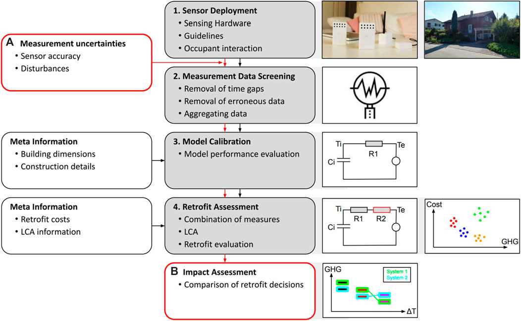
FIGURE 1. Process of measurement uncertainty impact assessment (red frame) based on the evidence-based retrofit process (black frame).

In this process, uncertainties can occur during the data acquisition through measurement inaccuracies or disturbances. These uncertainties are present in the raw data, which are processed in step 2, where additional inaccuracies can be introduced during data aggregation. In order to assess the impact of such uncertainties in the measurement data, distortions were simulated by synthetically adding variations to a dataset with presumably little distortions. The form and range of these synthetic distortions are based on experience from previous studies where sensors were deployed in occupied buildings (Frei et al., 2020; Frei et al., 2021) and on comparisons of measurement data from different sensors. After the insertion of the synthetic distortions, the retrofit process continues and yields a set of performance indicators for potential retrofit measures to be applied to the building. The impact of the synthetic distortions can be assessed by comparing the different sets of performance indicators resulting from each input dataset.

Sensor Deployment and Data Screening

The first step of the process is the creation of measurement data to capture the envelope-based heat loss calculation. For data acquisition, a lean open-source WSN was used for the in-situ measurements. It was introduced in a previous publication, where the cost, performance, and choice of sensors are discussed in detail (Frei et al., 2020). The sensor node installation took on average 12 min. The cost per node ranges from approximately 116 USD (air temperature and humidity) to 1,800 USD (water flow meter). All design files for the hardware and the software of the WSN are available online¹. The deployment process is described in detail in (Frei et al., 2020; Frei et al., 2021). Sensor data collection provides the foundation for the creation of the resistance-capacitance modeling process.

Building Envelope Resistance-Capacitance Modeling

These measurement data are used to estimate parameters of a building model. In (Sigrist et al., 2020), a grey-box model based on a resistor-capacitor (RC) network was introduced. Within this framework, measurement data and geometric information are used to calibrate a single-zone RC model. The R and C parameters typically are estimated by means of a maximum likelihood estimation. It is important to check whether a strong correlation exists between the estimated parameters and the observed measurements. Once the model is calibrated to match the estimated with the measured parameters, the internal air temperature as well as the heating demand, and the effects of potential envelope retrofit measures on the heating demand can be obtained. The same model structure could be used with measurement data from different buildings of the same type. Measurement inputs include the external air temperature (T_e), the ground temperature (T_gr), solar heat input through windows (φ_sol) and on external surfaces (φ_re), and the heat input from the central heating system (φ_h). The heat input is derived from the supply temperature (T_s), the return temperature (T_r), and the water volume flow rate (V˙) of the heating system.

The grey-box model parameters represent the heat transfer coefficients of the building envelope, the thermal mass of the building, and heat transfer coefficients of the heating system. However, changes to thermal mass and heat emission systems are not considered. Only changes to the envelope parameters and heat generation are considered.

The measurement of the indoor air temperature (T_i) is used for the model output. The model output is used to evaluate the predictive power of the grey-box model. For cross-validation, the measurement data is split into two subsets. The training dataset is used during the grey-box model parameter estimation process. During this process, the grey-box model parameters are varied in such a way, as to minimize the error between the predicted indoor temperature and the measured indoor temperature from the training dataset. The validation dataset is then used to evaluate the grey-box model with estimated parameters. During the validation, the error between predicted indoor temperature and measured indoor temperature is used as a model performance metric. For the sake of simplicity, we focus in this work on the mean absolute percentage error (MAPE, Eq. 1).

$MAPE\left(T_i\right)=\frac{1}{n}{\displaystyle \sum }_{j=1}^n\left|\frac{T_{i, mes, j}-T_{i,pre,j}}{T_{i, mes, j}}\right|(1)$

where T_i,mes,j is the measured indoor temperature at timestamp i. T_i,pre,j is the indoor temperature predicted by the grey-box model at timestamp j, and n is the number of all timestamps. In the context of building control, the actual estimates of the model parameters would be of less interest, as long as the model has great predictive power (small MAPE). In the context of this work, the purpose of the grey-box modeling is to acquire estimates of building characteristics, e.g., HLC, that are physically meaningful and as close to the true values as possible. However, the true value is unknown and can only be approximated for real buildings. Hence, we need to resort to the MAPE of the indoor temperature, get an indication of how good the model can recreate measured data, and assuming that good prediction of the indoor temperature also indicates meaningful model parameters. It is possible that a grey-box model yields meaningful estimates for model parameters while maintaining low predictive power.

Building Envelope Intervention Modeling

Model parameters of the calibrated RC model can be altered to emulate retrofit measures applied to the building envelope. The type of retrofit measures includes roof insulation, wall insulation, cellar ceiling insulation, and window replacement. The modified model parameters are calculated based on the estimated value from the model generation and the U-value of the retrofit measure. For instance, if additional insulation is to be applied to the walls, the new U-value U_new of the walls with insulation is calculated according to Eq. 2.

$U_{new}=\frac{1}{\left(1/U_{old}\right)+\left(1/U_{retrofit}\right)}(2)$

where U_old is the U-value of the walls of the existing building and U_retrofit is the U-value of the additional layer of insulation. The additional thermal capacity of the retrofit measures is neglected. The heat loss coefficient is calculated as the weighted sum of all heat transfer coefficients from the indoor temperature node to the environment. The calibrated model with the applied retrofit measures can be used to simulate the hourly heat demand of the post-retrofit building for a reference year. This simulation is carried out for all permutations of the retrofit measures.

Heating System Modeling

Once the building RC-model is generated, the modeling of the heating system is performed. In this framework, the heating system entails only the heat generation system. The heat emission system is considered as part of the building RC-model and is mentioned above. This step is important in the context of Switzerland, where a large share of energy in buildings is consumed for space heating (Kemmler and Spillmann, 2020). The retrofitting options for sizing the heating system are based on the heating load, which is based on the HLC and design temperatures for the indoor and outdoor. Each combination of retrofit measures requires an individual sizing of the heating system accordingly.

Heating System Sizing

The first step in the system modeling process is the system sizing based on the output of the RC-model derived from the sensor measurements. The maximum heating capacity Φ_h,max is the sum of the design space heating load and the heat demand for domestic hot water (Q_DHW) as seen in Eq. 3). The design space heating load is represented by the multiplication of the HLC of the model and the design values for the internal and external temperatures, i.e., T_i,design and T_e,design.

${\Phi }_{h,\max }=HLC\cdot \left(T_{i,design}-T_{e,design}\right)+\frac{Q_{DHW}}{8760h}(3)$

The heat demand for DHW is based on the local standard SIA 2024 (Swiss Society of Engineers and Architects (SIA), 2015), where Q_DHW is assumed to be constant throughout the year. For pellet boilers and district heating, a fixed heating efficiency independent of the envelope configuration and season was assumed. Thus, the final energy demand for space heating and DHW FED_h&DHW [kWh/a] is calculated as:

$FE{D}_{h\&DHW}=\frac{Q_h+\left(Q_{DHW}/{\eta }_{DHW}\right)}{{\eta }_h}(4)$

For heat pump-based heating system, the seasonal performance factors need to be considered. The detailed equations for the sizing of heating systems based on heat pumps are available in Supplementary Appendix A.

Life-Cycle Assessment Process

The projected energy consumption of a heating system is useful to determine operational efficiency, but retrofit decisions also need to address cost-effectiveness and greenhouse gas emissions. Thus, we include both as a metric for assessing the retrofit options. In the following subsection, we provide the details for both metrics.

Cost Assessment

The foundation of the calculation of the life-cycle costs is based on the assessment of the global cost (GC) outlined by (EU Commission, 2012), which has been used in other building retrofit assessments, e.g., (Tadeu et al., 2015). Equation 5 outlines the calculation of the global cost.

$GC\left(\tau \right)={\displaystyle \sum }_{i=1}^{m}I{C}_i+{\displaystyle \sum }_{t=1}^{\tau }\frac{EC\left(t\right)}{{\left(1+\left(r/100\right)\right)}^t}+{\displaystyle \sum }_{t=1}^{\tau }\frac{OMC}{{\left(1+\left(r/100\right)\right)}^t}+{\displaystyle \sum _{i=1}^m{\displaystyle \sum _k\frac{R{C}_{i,k}}{{\left(1+\left(r/100\right)\right)}^k}}}-{\displaystyle \sum }_{i=1}^m\frac{V_i\left(\tau \right)}{{\left(1+\left(r/100\right)\right)}^{\tau }}(5)$

where m is the number of measures. τ [a] is the calculation period. r [%] represents the real interest rate. IC_i [CHF] stands for the investment cost of the measure i and V_i(t) represents the residual value of measure i after the calculation period τ. EC(t) [CHF/a] is the energy cost in the year tt and OMC [CHF/a] represents the operation and maintenance cost. RC_i,k is the replacement cost of measure i at the end of its lifetime LT_i in year k where k = n·LT_i< τ for n = 1, 2, 3,....

The Energy cost EC(t) [CHF/a] is calculated as

$EC\left(t\right)=FE{D}_{h\&DHW}\cdot P_{ec}\cdot {\left(1+\frac{r_{ec}}{100}\right)}^t(6)$

where P_ec [CHF/kWh] is the energy price of the corresponding energy carrier ec. r_ec represents the annual change in energy price.

Greenhouse Gas Assessment

Cost has an impact on the retrofit-decision-making process. However, many individuals and organizations have a mandate to reduce greenhouse gas emissions. The greenhouse gas emissions calculation in this process is based on the ISO 14040 (International Organization for Standardization, 2006). Equation 7 outlines its calculation method.

$EI={\displaystyle \sum }_{i=1}^m\left(\frac{E{I}_{embodied,i}}{L{T}_i}\right) +FE{D}_{h\&DHW}\cdot C{F}_{EI,ec}(7)$

In Eq. 7, the unit of measurement for the environmental impact (EI) is kg-CO₂-equivalents according to the IPCC 2013GWP 100a method. For the materials used, the production and disposal of the used materials are considered along with the transport from the factory to the construction site. The processing on the construction site, and the maintenance of the heating system and building envelope were neglected.

Measurement Uncertainties Quantification and Analysis

The focus of this study is to calculate the impact of sensor measurement uncertainty on the retrofit decision, which results in implications on the final life cycle cost and greenhouse gas emissions. This process is done through the modulation of various sensor measurement data parameters to calculate the propagation of those errors into the retrofit metrics and, therefore, the retrofit decision-making process. Figure 2 exemplary illustrates a schematic of the process to test the influence of indoor air temperature measurement uncertainty on the heating load and HLC. First, the original (unaltered) data set is afflicted with additional synthetic errors according to estimated and previously observed measurement uncertainties. The altered data set is then fed into the RC model estimation process to estimate the RC-model parameters. The output of this step is an estimate of the overall HLC and model performance indicators such as the mean absolute percentage error (MAPE) for the indoor temperature. The MAPE of the model output indicates how well the RC model is able to predict the indoor temperature. Following, the retrofit measures are applied to the model, which means that the model parameters are altered to emulate the retrofit interventions. This altered model is then used to predict the yearly heating energy demand of the refurbished building and the required supply temperatures of the heating system. In the next step based on heating load, heating systems can be sized, and the heating demand can be converted into final energy demand. Environmental impact assessment and cost assessment are then done based on the applied envelope measures, system sizing, and final energy demand.

FIGURE 2

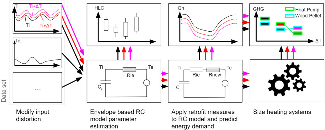
FIGURE 2. Process diagram of calculating the propagation of sensor measurement uncertainty error on the impact assessment of retrofits. The red and magenta lines represent the synthetically distorted measurement data.

In Table 1, we present an example of potential causes of uncertainties along with their impact. The data was derived from previous experiences (Frei et al., 2020; Frei et al., 2021). The sensor accuracies are taken from the manufacturers’ datasheet. The last column lists how original data was altered (modulation) in order to emulate all uncertainties.

TABLE 1

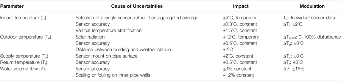
TABLE 1. Overview of measurement uncertainties and the corresponding sources.

The unaltered indoor temperature T_i input of the RC model consists of all indoor temperature measurements averaged and weighted by the volume of the room where the sensors were placed. However, as it would reduce the measurement effort and simplify the WSN, the measurement data of just one indoor temperature sensor (T_i,i) is used instead. From the raw data of this and previous work (Frei et al., 2021), it is visible that measured indoor temperatures often exhibit similar trends, while the main difference is a relatively constant offset. Such temperature offsets, albeit smaller, could also be caused by an offset error of the sensor. To emulate these effects, the averaged indoor temperature data is afflicted with an offset of ±2°C in order to emulate the sensor accuracy and thermal stratification effects (T_i + ∆T_i).

The outdoor temperature (T_e) is also modulated in two ways; First, we emulate distortions caused by solar radiation on shaded and unshaded outdoor temperature sensors. Second, we emulate errors caused by sensor offsets and offsets due to differences between temperature data measured on-site and data measured by a nearby weather station. Differences in elevation and the urban heat island effect can cause differences in the outdoor temperature data (Frei et al., 2021). To emulate the solar distortion, a weighted average is formed of the measurements from a shaded temperature sensor and one exposed to the sun (T_e + ∆T_e,sol). The weight is increased from 0 to 100%, in steps of 20%. The 0% data consists only of data from the shaded sensor, and 100% represents data from only the sensor affected by solar radiation. For the sake of simplicity, the second modulation consists of constant offsets between ±3°C in order to emulate sensor accuracy and distance between the building and the sensor, e.g., data from nearby weather stations.

The two main sources of measurement uncertainties for the supply and return temperature (T_s, T_r) are the sensor mount and sensor accuracy. While the temperature of interest is the fluid temperature, with the current setup only the pipe temperature is measured. Hence, these temperatures are modulated with an offset of ±2°C (T_s + ∆T_s, T_r + ∆T_r).

Lastly, the water flow rate measurement ($\dot{V}$) is afflicted by sensor accuracy and scaling or fowling on the inner pipe surface. The pipes from the case study building have an inner diameter of 33.7 mm. A 1 mm layer of fouling would reduce the cross-sectional area by 12%. Hence, the flow data is afflicted with offsets of ±15% ($\dot{V}$ + ∆$\dot{V}$).

Case Study Implementation

To demonstrate the application of the proposed process, a case study was chosen. The process was deployed on a single-family residential building in the city of St. Gallen, Switzerland, during the heating season 2018–2019. The key building properties are available in Table 2.

TABLE 2

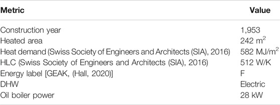
TABLE 2. Overview of the case study building properties.

Figure 3 shows the case study building and the floor plans. There are four occupants living in the building. The building underwent several refurbishments. A non-condensing oil boiler was installed in 1990. Water is used as the heating distribution medium through a system of radiators, which are controlled by thermostatic valves.

FIGURE 3

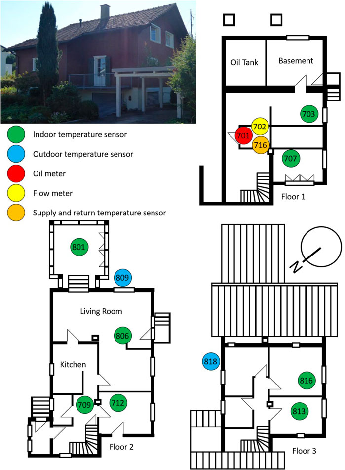
FIGURE 3. Case study overview: a recent photo of the residential building case study in St. Gallen, Switzerland (left, view from west) and the floor plans with indications of where various sensors were installed.

The case study building is typical for Switzerland, where 57% of all residential buildings are single-family buildings and 51% of all buildings were built before 1970 (Bau-und Wohnungswesen 2018, 2020). Further, 89% of residential buildings have a central heating system, and 60% of residential buildings use fossil fuels as a primary source for heating².

All sensor types used for this work are listed in Table 3. The measurement data were acquired with a sampling interval of 5 min. Based on the insight from previous work (Frei et al., 2021), the sensor suite was extended by an ultrasonic clamp-on flow meter (Keyence FD-Q-32C) for this work. Such a flow meter allows measuring the space heating input independent of the primary energy carrier and domestic hot water (DHW) generation. Unfortunately, the electricity demand could not be measured with the WSN in this building because the whole house energy meter did not have an interface that allowed access to it. However, the electricity demand was read manually from the electricity meter at the beginning and at the end of the measurement campaign.

TABLE 3

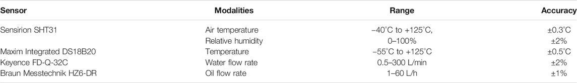
TABLE 3. Overview of sensors deployed in the case study with the corresponding accuracy ranges from their documentation.

The sensor deployment lasted from January 28 to April 17, 2019. During the 79 days of deployment, three major interruptions occurred, splitting the entire dataset into two larger sets, each lasting 22 days (February 09–March 03, March 06–March 28). The average data loss rate for these two datasets was 0.44%. The total electricity demand amounts to 10% of the total energy input. Based on previous experience (Deb et al., 2019) and the absence of electrical heaters for space heating, we assume that a significant amount of this electricity is used for DHW generation, which does not contribute to space heating. Hence, it appears to be acceptable to neglect electricity as heat input for space heating.

Tested Retrofit Measures

We selected a series of typical retrofit configurations with various combinations of retrofit options that, in a previous analysis, have shown to be cost-optimal for the case study building. These options are primarily variations of the building’s insulation type, material, and thickness (Sigrist et al., 2019):

• 20 cm mineral wool inter-rafter roof insulation (0.18 W/m²K).

• 16 cm polystyrene ventilated curtain facade insulation (0.19 W/m²K).

• 16 cm mineral wool cellar ceiling insulation (0.19 W/m²K).

• Triple-glazed windows replacement (0.76 W/m²K).

Table 4 illustrates the combination of envelope-based retrofit options that were tested in the case study. Each envelope option was applied to the four heating system types being considered in this context: wood pellet boilers, district heating, air-to-water heat pumps, and geothermal heat pumps.

TABLE 4

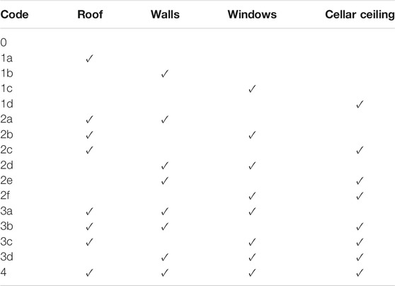
TABLE 4. Combination of building envelope-based retrofit measures implemented on the case study with the corresponding unique identifying codes used in subsequent figures (adapted from Sigrist et al. (2020))

The retrofit options for upgrading the heating system include wood pellet boilers, district heating, ground source heat pumps, and air-to-water heat pumps. The design parameters used for the sizing of the interventions, environmental impact assessment, and cost assessment are available in Supplementary Appendix B.

Results and Discussion

After the implementation of the methodology on the case study, the results are presented in this section to illustrate the impact of measurement errors on the decision-making process. The impact of the error propagation on the heat loss coefficient is outlined, followed by the result on the overall systems retrofit analysis according to the life cycle cost and greenhouse gas emissions.

Sensor Error Impact on Parameter Estimation

First, we compare the output of the RC model with the measurement data. The MAPE for the indoor temperature during the validation period amounts to 3.9%. This represents a mean temperature error of 0.86°C, which is common. The building characteristics derived from the measurement or from the RC model deviate in part significantly from the building characteristics estimated according to the standard (SIA 380/1). For example, the unaltered data set yields 485 W/K as an estimate for the overall HLC, compared to an HLC of 512 W/K estimated by the standard-based assessment. This represents a 5.5% difference.

Second, we compare the annual heating demands derived with three different methods. According to the calculations using the standard (SIA 380/1), the annual heating demand is 39,170 kWh/a, while the RC model predicts an annual heating demand of only 28,630 kWh/a. The measured oil consumption normalized by heating degree days amounts to a heating demand of 30,660 kWh/a. An assumed boiler efficiency of 90% yields a heating demand of 27,594 kWh/a. Hence, the standard-based heating demand deviates by 40% from the measured heating demand, while the heating demand based on the RC model deviates by 2.4% from the measurement. Hence, the RC model yields a significantly more accurate heating demand than building energy assessment according to the local standard.

Figure 4 shows the impact of measurement disturbances on the estimation of the HLC (A) and the MAPE of the indoor temperature (T_i) (B). The variation of the HLC estimates shows how robust the proposed grey box model is against measurement uncertainties. In other words, it shows how robust this method of building performance assessment is against measurement errors. The HLC estimates range from 343 W/K (−29%) to 590 W/K (+22%). Most notably, the impact of solar disturbance of the outdoor temperature measurement on the estimation of the HLC is moderate, with a maximum deviation of 3%.

FIGURE 4

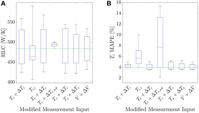
FIGURE 4. Selected input parameters together with measurement uncertainty impact on the HLC (A) and model quality (B). The green line indicates the performance based on the unaltered dataset.

The variations in the MAPE of the indoor temperature indicate how robust the predictive power of the proposed RC model is against disturbances in the measurement data (Figure 4B). For a moderate solar impact of 20%, the MAPE of T_i even improves. However, for cases with stronger solar disturbance, the MAPE of the indoor temperature of the resulting models deteriorates drastically. It is an overall trend that small spreads in HLC estimates come with a larger spread in T_i-MAPE. Further, the MAPE in the presence of measurement error stays robust for the parameters of outdoor temperature (T_e) and sensors for the heating system (T_r, T_s, $\dot{V}$).

A possible explanation is that when the model is able to capture the dynamics of the altered data sets, the model parameters change, and the modeling error remains small. In cases where the model estimation process is not capable of capturing the dynamics of the dataset, the model parameter estimation is dominated by initial values, and the model has little predictive power. Hence, the HLC spread remains small, and the predictive error (MAPE) becomes large. Exemplary for this is the results for the outdoor temperature disturbed by solar radiation T_e,solar. Solar radiation causes the apparently measured temperature values to rise and fall much steeper than usual. These measurement distortions occur only during sunny hours. During these periods, the heating load is small because the solar radiation also increases the true ambient temperature, and hence the temperature difference between indoor and outdoor is smaller. From a steady-state perspective, it is in any case difficult to estimate the HLC during the day because a small heating load is divided by a small temperature difference. In this scenario, any deviations in the numerator and denominator have a larger impact on the results, making it noisier. On the other side, during the night or during cloudy days, the heating load is larger, and the temperature difference between indoor and outdoor is larger. Hence, deviations from the true values have a smaller impact on the results. Therefore, estimates during these periods are more reliable and heavier weighted in the estimation process. Hence, the spread of HLC estimates is small, but the predictive power of the model deteriorates significantly. This could indicate that, in the case of solar radiation impacting outdoor temperatures, the model would perform poorly for control purposes. However, it yields robust results for building performance assessment.

Table 5 relates the impact of the measurement uncertainties from Table 1 on HLC estimates with the magnitude of the measurement uncertainty. This is done by dividing the difference between the largest and smallest HLC estimates by the difference of the most positive and the most negative modulation of measurement data. This method yields a measure of the sensitivity of the HLC estimate regarding measurement uncertainty. It shows that the HLC estimation is most sensitive for measurement errors of the water flow rate measurement of the heating system.

TABLE 5

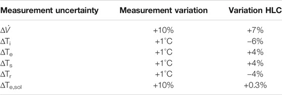
TABLE 5. Sensitivity of the HLC to measurement errors.

Retrofit Measure Performance Impact Due to Sensor Error

Figure 5 shows an overview of the range of intervention measures implemented for the case study. The box for each retrofit combination is labeled according to system and retrofit code from Table 4. Two boxes of the same retrofit configuration are connected if their rank changes from one measurement offset to the next one. The distance between the various retrofit configurations is highly influenced by the underlying assumptions. In the presented case study, an emission factor of 0.108 kg-CO₂/kWh was assumed for district heating. This results in a lower performance compared to the other systems, which are assumed to be driven by local resources (0.027 kg-CO₂/kWh) or electricity from the Swiss grid with a rather low carbon intensity of (0.102 kg-CO₂/kWh), which is further leveraged by the performance factors of the heat pumps. As a consequence, all district heating configurations are distant from other configurations in regard to greenhouse gas emissions. The rank of different envelope configurations does not change for district heating, regardless of the measurement input. Generally, the ranking of a retrofit configuration only changes if performance is very close to the performance of another configuration.

FIGURE 5

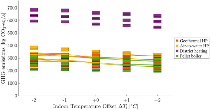
FIGURE 5. Measurement uncertainty impact on the predicted performance of retrofit measures in absolute numbers, which show a general downwards trend from left to right and are close in terms of grouping of the most retrofit measure combinations. Rank changes of retrofit measure combinations due to measurement uncertainty indicated with lines between the boxes occur rarely.

To better visualize the impact of potential measurement uncertainties on predicted relative performance and retrofit decisions, the various configurations are listed by their rank. In the presented example, the best performing solutions in terms of GHG solutions are using a wood pellet boiler (Figure 6). No changes in ranks are observed, i.e., these solutions seem to be robust against the investigated indoor temperature offsets. Changes in ranks are only observed for configurations that perform similarly. This illustrates the change of order of the interventions that can occur for measurement uncertainties of the indoor temperature. Boxes of the same retrofit configuration are connected between two measurement offsets if the rank of the retrofit configuration changes. While absolute differences are not visible in this plot, rank changes are apparent. Notably, the five best performing retrofit configurations do not change regardless of the measurement offset. These retrofit configurations are based on wood pellets and geothermal heat pump systems combined with minimal or no measures applied to the envelope.

FIGURE 6

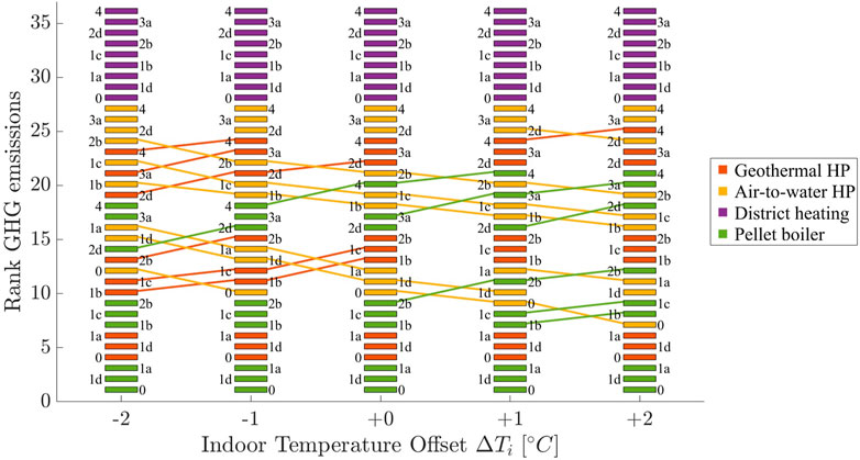
FIGURE 6. Measurement uncertainty impact on the rank of predicted performance of retrofit measures. The changes is ranks are small with one or two positions at maximum.

Figure 7 provides an overview of how various measurement uncertainties impact the greenhouse gas emissions (Figure 7A) and the global cost (Figure 7B) of the retrofit interventions. Generally, the trend is similar for greenhouse gas emissions and global costs. If a positive measurement offset results in increased greenhouse gas emissions, the global costs will also increase and vice versa. While retrofit interventions in including district heating are far off from the other inventions with regards to greenhouse gas emissions, district heating solutions are in the midst of retrofit interventions regarding cost. Instead, wood pellet boiler solutions with no envelope interventions stand apart due to high global costs. Similarly, retrofit interventions with little changes to the envelope and a geothermal heat pump stand apart on the low side of costs. These distinct gaps are independent of the magnitude of measurement uncertainty or affected measurement input.

FIGURE 7

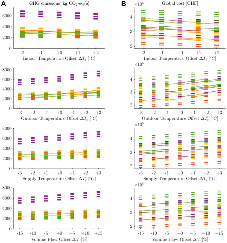
FIGURE 7. Measurement uncertainty impacts from various measurement uncertainties on the rank of predicted performance of retrofit measures, (A) greenhouse gas emissions, (B) global cost, red: geothermal heat pump, yellow: air-to-water heat pump, purple: district heating, green: pellet boiler. All plots show that the spacing between the retrofit measures combinations remains similar throughout out the input variation and the changes in ranks are rare and are limited to one or two positions.

It is apparent that measurement uncertainties have little impact on the retrofit decision, i.e., the rankings in terms of cost and GHG emissions of retrofit interventions only change in few cases. In cases where a reordering occurs, the interventions that switch ranks perform very similarly. However, the measurement uncertainties can have a significant impact on absolute performance, i.e., absolute cost and GHG emissions. Hence, the management of measurement uncertainty is particularly important for the sizing of retrofit measures and achieving energy saving targets.

Retrofit decisions are commonly based on a multi-criteria analysis, where several performance parameters, including costs and GHG emissions, are considered simultaneously. We chose to present the range of uncertainties in a scatter plot, where the range of the performances (GHG, cost) of retrofit measures is indicated by ellipses (Figure 8). The centers of the ellipses indicate the performance of the retrofit interventions using the unaltered data set. The length of the ellipse axes is based on datasets, where measurement errors were applied to every measurement input in such a way to produce a very high estimate for the HLC and a very low estimate of the HLC.

FIGURE 8

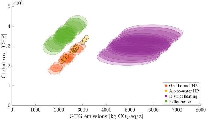
FIGURE 8. Uncertainty ranges illustrated in the context of energy consumption and its implications on cost and GHG emissions.

In Figure 8 one can observe that the impact of measurement uncertainty on costs and emissions are mostly dependent on the exchange of the heating system. Differences based on the envelope configuration are negligible. The impact on cost and emissions is noticeably larger for wood pellet boiler and district heating systems. After considering the system efficiencies and performance factors, these two systems have the highest energy cost of heat production at 0.11 CHF/kWh and 0.09 CHF/kWh. In comparison, air-to-water heat pumps cost 0.07 CHF/kWh. For geothermal heat pumps, it is 0.05 CHF/kWh.

District heating has the largest GHG emission intensity. This effect is further elevated when considering system efficiencies and performance factors. A share of the GHG emissions of geothermal heat pumps depends on the length of the borehole, which is sized based on the HLC. Hence, the variable share GHG emissions for geothermal heat pumps increases the impact of measurement uncertainties on GHG emission estimates. Likewise, the uncertainty of costs for geothermal heat pump based systems is driven by the high variable investment costs for geothermal heat pumps.

The RC-models used to produce Figure 8 performed poorly with MAPE for T_i of 16 and 63%. The HLC estimation yielded 290 and 590 W/K, respectively. Notably, the uncertainties for cost and GHG estimates are much more pronounced for district heating systems and pellet boiler systems, while the effect for heat pump-based systems is moderate.

In Sigrist et al. (2020), it was shown that the RC model is able to predict the indoor temperature adequately with unaltered measurement data. But when all measurement inputs are maximally distorted to form worst-case scenarios, the RC model is no longer able to predict the indoor temperature adequately and the HLC estimates are far off. Hence, we could hypothesize that poor RC model performance indicates poor data quality, provided that the model structure is adequate.

Conclusion

This paper outlines a novel process of using sensor-driven RC models and parametric analysis to quantify the impact of measurement uncertainty, exemplified in a residential case study in Switzerland. A four-step process was implemented to deploy various sensors, screen the data for quality, create the RC models using building meta-data, and conduct the retrofit assessment according to both life cycle cost and GHG emissions. The framework created from this process was then subjected to a series of perturbations of the input data to emulate measurement uncertainty, and the impact on the output metrics was quantified. The results illustrate that for all configurations, the impact of measurement uncertainty is manageable. In some configurations, such as district heating and wood pellet boiler systems, the impact was greater, while measures that utilized heat pump systems, were affected less. For the presented case study, individual measurement uncertainties appear to have little impact on the retrofit decision, i.e., the ranking of retrofit interventions with regard to costs or emissions is little affected by measurement errors. However, in a worst-case scenario with all measurement uncertainties compounding towards the same sign of the error, the RC model fails, and the estimated building properties become unreasonable. As a consequence, the prediction of retrofit measures appears to be futile. For cases where the RC-model showed apparently reasonable results from a data set with significant synthetic errors in the range observed measurement uncertainties, absolute performance results showed deviations of 3–26%. Thus, measurement uncertainties should be paid attention to when one is concerned with building systems, e.g., sizing of the heating systems. Further, measurement uncertainties are also important for achieving the predicted performance targets of a building refurbishment. Hence, measurement uncertainties should be kept to a minimum to narrow the performance gap of refurbishments. For example, higher accuracy temperature sensors and appropriate measures against solar disturbances should be implemented. At the current state of this work, the performance of the case study building with implemented retrofit measures has not yet been demonstrated because no retrofit measures have yet been implemented. Also, so far the methods have been applied to Swiss single-family buildings only, and the retrofit assessment entails retrofit measures typically applied in Switzerland. Therefore, it is still to be investigated how these methods can also be applied to other building types, different climates, and geographical contexts.

Data Availability Statement

The raw data supporting the conclusion of this article will be made available by the authors, without undue reservation.

Author Contributions

MF carried out the measurements, carried out the impact assessment, wrote the first draft of the manuscript, contributed to the conception and design of the study. IH wrote the first draft of the manuscript, contributed to the conception and design of the study. CD established the RC modeling framework, including systems and LCA, wrote the first draft of the manuscript. DS established the RC modeling framework, including systems and LCA. AS contributed to the conception and design of the study. All authors contributed to manuscript revision, read, and approved the submitted version.

Funding

This work was financially supported by the Office for Water and Energy of the Canton St. Gallen. This research project is financially supported by the Swiss Innovation Agency Innosuisse and is part of the Swiss Competence Center for Energy Research SCCER FEEB&D.

Conflict of Interest

The authors declare that the research was conducted in the absence of any commercial or financial relationships that could be construed as a potential conflict of interest.

Acknowledgments

We would like to thank Enrico Romano and John Bruggmann of Gerevini Ingenieurbüro AG for sharing their assessment of the case study buildings. Further, we would like to thank the participants of the case study, who allowed us to place sensors in their homes. Moreover, we are grateful to Krishna Bharathi for the fruitful discussion.

Supplementary Material

The Supplementary Material for this article can be found online at: https://www.frontiersin.org/articles/10.3389/fbuil.2021.675913/full#supplementary-material

Footnotes

¹https://github.com/architecture-building-systems/Wireless-Sensor-Network.

²https://www.bfs.admin.ch/bfs/en/home/statistics/constructionhousing/buildings/energy-field.html.

References

Almeida, M., and Ferreira, M. (2018). Ten Questions Concerning Cost-Effective Energy and Carbon Emissions Optimization in Building Renovation. Building Environ. 143, 15–23. doi:10.1016/j.buildenv.2018.06.036

CrossRef Full Text | Google Scholar

Alzetto, F., Pandraud, G., Fitton, R., Heusler, I., and Sinnesbichler, H. (2018). QUB: A Fast Dynamic Method for In-Situ Measurement of the Whole Building Heat Loss. Energy and Buildings 174, 124–133. doi:10.1016/j.enbuild.2018.06.002

CrossRef Full Text | Google Scholar

Bau- und Wohnungswesen 2018 (2020). Neuchâtel: Bundesamt für Statistik (BFS). Available at: https://www.bfs.admin.ch/hub/api/dam/assets/12507412/bibtex.

Google Scholar

Bauwens, G., and Roels, S. (2014). Co-heating Test: A State-Of-The-Art. Energy and Buildings 82, 163–172. doi:10.1016/j.enbuild.2014.04.039

CrossRef Full Text | Google Scholar

Cozza, S., Chambers, J., Deb, C., Scartezzini, J.-L., Schlüter, A., and Patel, M. K. (2020). Do energy Performance Certificates Allow Reliable Predictions of Actual Energy Consumption and Savings? Learning from the Swiss National Database. Energy and Buildings 224, 110235. doi:10.1016/j.enbuild.2020.110235

CrossRef Full Text | Google Scholar

Deb, C., Frei, M., Hofer, J., and Schlueter, A. (2019). Automated Load Disaggregation for Residences with Electrical Resistance Heating. Energy and Buildings 182, 61–74. doi:10.1016/j.enbuild.2018.10.011

CrossRef Full Text | Google Scholar

Dimitriou, V. (2016). Lumped Parameter thermal Modelling for UK Domestic Buildings Based on Measured Operational Data. Available at: https://dspace.lboro.ac.uk/dspace-jspui/handle/2134/23239 (Accessed March 11, 2017).

Google Scholar

EU Commission (2012). Commission Delegated Regulation (EU) No 244/2012 of 16 January 2012 Supplementing Directive 2010/31/EU of the European Parliament and of the Council on the Energy Performance of Buildings. Official J. Eur. Union 55, 18–36.

Google Scholar

Frei, M., Deb, C., Nagy, Z., Hischier, I., and Schlueter, A. (2021). Building Energy Performance Assessment Using an Easily Deployable Sensor Kit: Process, Risks, and Lessons Learned. Front. Built Environ. 6. 609877. doi:10.3389/fbuil.2020.609877

CrossRef Full Text | Google Scholar

Frei, M., Deb, C., Stadler, R., Nagy, Z., and Schlueter, A. (2020). Wireless Sensor Network for Estimating Building Performance. Automation in Construction 111, 103043. doi:10.1016/j.autcon.2019.103043

CrossRef Full Text | Google Scholar

Galimshina, A., Moustapha, M., Hollberg, A., Padey, P., Lasvaux, S., Sudret, B., et al. (2020). Statistical Method to Identify Robust Building Renovation Choices for Environmental and Economic Performance. Building Environ. 183, 107143. doi:10.1016/j.buildenv.2020.107143

CrossRef Full Text | Google Scholar

Global Alliance for Buildings and ConstructionInternational Energy Agency and the United Nations Environment Programme (2019). 2019 Global Status Report for Buildings and Construction: Towards a Zero-Emission, Efficient and Resilient Buildings and Construction Sector. Available at: https://webstore.iea.org/download/direct/2930?fileName=2019_Global_Status_Report_for_Buildings_and_Construction.pdf.

Google Scholar

Hall, M. (2020). Normierung des GEAK®. Konferenz Kantonaler Energiedirektoren. Available at: https://www.endk.ch/de/ablage/grundhaltung-der-endk/20200402_Normierung_GEAK_EnDK_D.pdf.

Google Scholar

Heo, Y., Augenbroe, G., Graziano, D., Muehleisen, R. T., and Guzowski, L. (2015). Scalable Methodology for Large Scale Building Energy Improvement: Relevance of Calibration in Model-Based Retrofit Analysis. Building Environ. 87, 342–350. doi:10.1016/j.buildenv.2014.12.016

CrossRef Full Text | Google Scholar

Heo, Y., Choudhary, R., and Augenbroe, G. A. (2012). Calibration of Building Energy Models for Retrofit Analysis under Uncertainty. Energy and Buildings 47, 550–560. doi:10.1016/j.enbuild.2011.12.029

CrossRef Full Text | Google Scholar

International Energy Agency and the United Nations Environment Programme (2018). 2018 Global Status Report: Towards a Zero-Emission, Efficient and Resilient Buildings and Construction Sector. Available at: https://wedocs.unep.org/bitstream/handle/20.500.11822/27140/Global_Status_2018.pdf.

Google Scholar

International Organization for Standardization (2008). ISO 13790:2008 - Energy Performance of Buildings - Calculation of Energy Use for Space Heating and Cooling. Geneva, Switzerland: International Organization for Standardization Available at: http://www.iso.org/iso/catalogue_detail.htm%3Fcsnumber=41974 (Accessed July 25, 2016).

International Organization for Standardization (2006). ISO 14040:2006 - Environmental Management - Life Cycle Assessment - Principles and Framework. Available at: https://www.iso.org/cms/render/live/en/sites/isoorg/contents/data/standard/03/74/37456.html (Accessed November 5, 2020).

Google Scholar

Kemmler, A., and Spillmann, T. (2020). Analyse des schweizerischen Energieverbrauchs 2000–2019 nach Verwendungszwecken. Bern, Switzerland: Swiss Federal Office of Energy Available at: https://www.bfe.admin.ch/bfe/de/home/versorgung/statistik-und-geodaten/energiestatistiken/energieverbrauch-nach-verwendungszweck.exturl.html/aHR0cHM6Ly9wdWJkYi5iZmUuYWRtaW4uY2gvZGUvcHVibGljYX/Rpb24vZG93bmxvYWQvMTAyNjA=.html.

Khoury, J., Hollmuller, P., and Lachal, B. M. (2016). Energy Performance gap in Building Retrofit: Characterization and Effect on the Energy Saving Potential.

Lee, S. H., Hong, T., Piette, M. A., and Taylor-Lange, S. C. (2015). Energy Retrofit Analysis Toolkits for Commercial Buildings: A Review. Energy 89, 1087–1100. doi:10.1016/j.energy.2015.06.112

CrossRef Full Text | Google Scholar

Ma, Z., Cooper, P., Daly, D., and Ledo, L. (2012). Existing Building Retrofits: Methodology and State-Of-The-Art. Energy and Buildings 55, 889–902. doi:10.1016/j.enbuild.2012.08.018

CrossRef Full Text | Google Scholar

Papafragkou, A., Ghosh, S., James, P. A. B., Rogers, A., and Bahaj, A. S. (2014). A Simple, Scalable and Low-Cost Method to Generate thermal Diagnostics of a Domestic Building. Appl. Energ. 134, 519–530. doi:10.1016/j.apenergy.2014.08.045

CrossRef Full Text | Google Scholar

Reid, E. (1984). Understanding Buildings: A Multidisciplinary Approach. Cambridge: MIT Press.

Rysanek, A. M., and Choudhary, R. (2013). Optimum Building Energy Retrofits under Technical and Economic Uncertainty. Energy and Buildings 57, 324–337. doi:10.1016/j.enbuild.2012.10.027

CrossRef Full Text | Google Scholar

Sigrist, D., Deb, C., Frei, M., and Schlüter, A. (2019). Cost-optimal Retrofit Analysis for Residential Buildings. J. Phys. Conf. Ser. 1343, 012030. doi:10.1088/1742-6596/1343/1/012030

CrossRef Full Text | Google Scholar

Sigrist, D., Deb, C., and Schlueter, A. (2020). A Calibrated RC Model for Dataxdriven Retrofit Analysis of a Residential Building. eSIM 2020-2021 Vancouver.

Google Scholar

Sunikka-Blank, M., and Galvin, R. (2012). Introducing the Prebound Effect: the gap between Performance and Actual Energy Consumption. Building Res. Inf. 40, 260–273. doi:10.1080/09613218.2012.690952

CrossRef Full Text | Google Scholar

Swiss Society of Engineers and Architects (SIA) (2015). SIA 2024:2015 Raumnutzungsdaten für die Energie- und Gebäudetechnik. Zürich: SIA.

Swiss Society of Engineers and Architects (SIA) (2016). SIA 380/1:2016 Heizwärmebedarf. Zürich: SIA.

Tadeu, S., Rodrigues, C., Tadeu, A., Freire, F., and Simões, N. (2015). Energy Retrofit of Historic Buildings: Environmental Assessment of Cost-Optimal Solutions. J. Building Eng. 4, 167–176. doi:10.1016/j.jobe.2015.09.009

CrossRef Full Text | Google Scholar

Tian, W., Heo, Y., de Wilde, P., Li, Z., Yan, D., Park, C. S., et al. (2018). A Review of Uncertainty Analysis in Building Energy Assessment. Renew. Sustain. Energ. Rev. 93, 285–301. doi:10.1016/j.rser.2018.05.029

CrossRef Full Text | Google Scholar