A Monte Carlo Simulation Approach in Non-linear Structural Dynamics Using Convolutional Neural Networks

1. Introduction

Deciding whether a structure subjected to ground motion is or is not safe is a delicate task in engineering. One big issue is the high level of uncertainty when considering a ground excitation time history relevant to structural design. This fact forces us to apply probabilistic methodologies to design structures and infrastructures (Der Kiureghian, 1996; Bucher, 2009).

Failure usually occurs in the non-linear range of structural behavior, making an analytic or closed form of the response statistics difficult or even impossible. In this context, the equivalent linearization method was proposed to approximate the response statistics, which is generally quite accurate around the mean of the distribution (Roberts and Spanos, 1990). To also provide accurate response statistics for infrequent events, the tail equivalent linearization method was proposed (Fujimura and Der Kiureghian, 2007).

The general Monte Carlo method is helpful to provide the response statistics of non-linear systems. The strategy is based on a series of computer experiments and provides an unbiased estimation for the probability of failure of a non-linear system (Hurtado and Barbat, 1998).

However, considering that each computer experiment includes a time history analysis of a complex high-dimensional finite element model, the Monte Carlo method turns out to be computationally expensive. As engineers, we have to ensure that structural failure should happen extremely rare, as it is generally accompanied by severe societal and economic loss. Thus, a disproportionately high number of computer experiments must be performed to estimate the occurrence of low-probability events with high confidence. This fact makes the application of the crude Monte Carlo method unfeasible for non-linear high-dimensional problems. A promising strategy to overcome this issue is to use model order reduction methods (Bamer and Bucher, 2012; Bamer and Markert, 2017; Bamer et al., 2018). This strategy enables one to decrease the computational burden for each sample computation significantly, and it is particularly efficient if only one reduced-order basis is applied during the whole Monte Carlo simulation run (Bamer et al., 2017).

In the context of computational speed-up and meta-modeling, the application of neural networks has proven to be a promising strategy (Stoffel et al., 2018, 2019, 2020a,b) for problems in non-linear structural mechanics. In particular, the incorporation of recurrent neural network architectures for elastoplastic problems leads to representations of the non-linear structural behavior revealing accurate and efficient solution functions (Koeppe et al., 2019, 2020).

With special emphasis on problems in earthquake engineering, Sun et al. (2021) has summarized the incorporation of machine learning approaches to response, damage, and failure prediction. Convolutional neural networks and deep learning have been used to predict the whole response time history of the structure subjected to a transient excitation (Zhang et al., 2020) and wavelet transformation-based response prediction (Lu et al., 2020, 2021; Liao et al., 2021). Thaler et al. (2021a,b) proposed a machine leaning-enhanced Monte Carlo method using a simple feed-forward neural network. In doing so, they used a selected choice of intensity measures from the time history data as a set of input parameters to predict the response of the structure. However, representing the whole time history data by a few hand-chosen scalar values only, much information regarding the excitation function can get lost.

In this paper, we present an extended Monte Carlo approach using convolutional neural networks so that it is not necessary to extract hand-designed input features, e.g., intensity measures, for the neural network. Furthermore, in order to assure high reliability of the neural network predictions in the tail of the distribution, an extended training strategy is applied.

The structure of this paper is goal-oriented and straightforward. In section 2, we firstly present an overview of convolutional neural networks followed by the presentation of the new Monte Carlo simulation strategy. Subsequently, in section 3, we present the new strategy using an illustrative numerical example. The efficiency, as well as advantages and disadvantages, are discussed. Finally, in section 4, the conclusion is drawn.

2. Methods

2.1. Feedforward and Convolutional Neural Network Architectures in a Nutshell

Machine learning strategies have been applied to a wide range of tasks in engineering. This section briefly introduces the basic theory of the two machine learning methods applied in this paper, i.e., feedforward and convolutional neural networks.

The feedforward neural network consists of at least three layers: input, hidden, and output layer. Every layer contains a set of neurons. The input layer receives the initial data. The data is passed forward, layer by layer, until the output layer is reached from this layer. Every neuron of a certain layer, which is not the output layer, is connected to every other neuron of the next layer during one forward step. As a result of this, each neuron-to-neuron link has its corresponding weight value. A weight matrix can then represent the set of all connections. Thus, the output of the previous layer y_i−1 is the input of the actual layer x_i. The input is then multiplied by the weight matrix W_i, and additionally, summed up by a bias vector b_i. The sum is transferred by an activation function f_act which is then the output y_i of a layer:

$\begin{array}{ll}{\text{y}}_i=f_{act}({\text{W}}_i{\text{x}}_i+{\text{b}}_i).& (1)\end{array}$

This operation is repeated until the output layer, which constitutes the prediction of the neural network. In our paper, we apply supervised learning, where the prediction is compared to a known target output for regression tasks. The error is used to optimize the weight matrices and the bias of all the layers using back-propagation.

The convolutional neural network is a specific type of architecture that is used to process data. It is specialized for input data that show a correlation of neighboring data points. Thus, typical applications of convolutional neural networks are image data. However, as presented during this paper, convolutional neural networks can also effectively be applied to extract the main features of earthquake time histories. Using convolutional layers improves the machine learning system by sparse interaction and parameter sharing. Consequently, a reduction of the total number of trainable parameters, and therefore, decreased computational effort. Convolutional neural networks are composed of two main operations: convolution and pooling.

The convolution is the basic mathematical operation of this neural network type. Regarding one dimensional discrete data, such as earthquake time histories for example, the convolution operation < * > of two vectors or one-dimensional tensors, g and h, is written as:

$\begin{array}{ll}{(\text{g}*\text{h})}_i={\displaystyle \sum _n}{g}_{i-n}{h}_n.& (2)\end{array}$

The convolutional operation is usually followed by a non-linear activation function f_act. The output y_i of the convolution operation, the so-called feature map, is written as:

$\begin{array}{ll}{\text{y}}_i=f_{act}({\text{x}}_i*{\text{w}}_i+{\text{b}}_i).& (3)\end{array}$

In this equation, w_i denotes a weight vector with the spatial size k of the kernel, which slides over the one-dimensional input data array x_i.

In the next step, pooling improves the statistical efficiency by reducing the spatial size of the data. As shown in Figure 1, pooling summarizes the input space. Looking at this illustrative example, one can see that the pooling procedure summarizes three values to one output value. As a result of this, the decrease in the total number of values, i.e., the compression of information, is dependent on the stride size, which is the step increment at which the kernel moves over the data array. For the example in Figure 1, the stride size is two. Two different types of pooling procedures are considered in this paper: max-pooling and average-pooling. As expected from the nomenclature, max-pooling extracts the maximum of all values within the moving kernel, and average pooling extracts the average of the values within the moving kernel. Even though convolutions and pooling are individual operations, it is often referred to as a convolutional layer, whereby the operations are carried out in different stages.

FIGURE 1

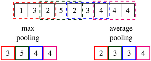
Figure 1. Exemplary spatial reduction of the top data array using pooling functions (pool size = 3, stride size = 2); output data reduced by maximum pooling (bottom left); output data reduced by average pooling (bottom right).

Similar to the weight optimization procedure of fully connected layers, the values of the convolutional kernels are optimized during training, which allows for the extraction of features of the input data. Different features can be extracted from the initial data by using multiple kernels within the convolutional layer. A convolutional neural network usually consists of several convolutional layers, followed by feedforward layers. The choice of the architecture depends on the complexity of the data and the task to solve (Kruse et al., 2015; Goodfellow et al., 2016).

2.2. Machine Learning Enhanced Monte Carlo Simulation

The probability of structural failure P_f can be expressed in terms of a multiple integral:

$\begin{array}{ll}{P}_f={\displaystyle \underset{g(\text{x})<0}{\int ...\int }}{f}_X(\text{x})\text{d}{x}_1...\text{d}{x}_n,& (4)\end{array}$

where g(x) is the limit state function that divides the entire domain into the save region g(x) ≥ 0 and the failure region g(x) < 0. Dependent on the complexity of the limit state function, the solution of this integral is generally not straightforward. However, one approach to solve this integral is provided by the Monte Carlo simulation. One performs a series of computer experiments by artificially generating a set of random inputs (Hurtado and Barbat, 1998). The integral describing the probability of failure in Equation (4) is rewritten as:

$\begin{array}{l}{p}_f={\displaystyle {\int }_{-\infty }^{\infty }{\displaystyle {\int }_{-\infty }^{\infty }...}}{\displaystyle {\int }_{-\infty }^{\infty }{I}_g}(x_1,...,x_n)\\ f_{X_1,...,X_n}(x_1,...,x_n)\text{ d}{x}_1...\text{d}{x}_n,& (5)\end{array}$

with I_g(x₁, . . . , x_n) being an indicator function defining a safe or failure state:

$\begin{array}{llll}{I}_g(x_1,...,x_n)=1\text{if }g(\text{x})& \le & 0\left(\text{structural failure}\right)& (6)\end{array}$

$\begin{array}{llll}{I}_g(\text{x})=0\text{if }g(\text{x})& >& 0\left(\text{save}\right).& (7)\end{array}$

Thus, the probability of failure is provided by a consistent unbiased estimate in terms of an expected value:

$\begin{array}{ll}{p}_f=\frac{1}{m}{\displaystyle \sum _{k=1}^m}{I}_g({\text{x}}^{(k)})\text{.}& (8)\end{array}$

The standard deviation of the estimation of the probability of failure is evaluated as:

$\begin{array}{ll}{\sigma }_{p_f}^2=\frac{p_f}{m}-\frac{p_f^2}{m}\approx \frac{p_f}{m}\Rightarrow {\sigma }_{p_f}=\sqrt{\frac{p_f}{m}},& (9)\end{array}$

which means that the variance of the probability of failure increases with a decreasing number of samples m. In engineering, we obviously want the probability of failure to remain a low value. Thus, the reliability of the estimate of a small probability of failure is considerably low using the Monte Carlo method and m must be chosen to be a disproportionately high number. In other words, extensive relevant earthquake record data must be collected in order to reliably design structures. A rule of thumb may be that a number of 10⁵ excitation records should be considered for structural design with a desired failure probability of 10⁻⁴—obviously an impossible task, as the number of recorded relevant ground excitations around the respective building site is inherently limited. Therefore, we suggest to artificially generate a sufficiently high number of random ground excitations using the metadata from one relevant record. In doing so, site-dependent structural design is possible. In order to realize artificial site-dependency, we consider the incorporation of a non-linear Kanai-Tajimi filter (Bamer and Markert, 2017). To extract the important information from a ground excitation record, a time window of size t_w is defined that moves over the excitation time history, as shown in Figure 2. For the numerical example in this paper, a severe earthquake, recorded in Kobe Takarazuka in 1995 (Kobe, 2016), is chosen as benchmark time history.

FIGURE 2

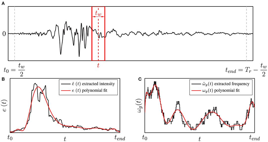
Figure 2. (A) Moving time window to extract relevant metadata from acceleration records; (B) extracted intensity and (C) extracted lowest frequency content.

In this paper, we extract two time-dependent identification parameters, which are the intensity ê(t) and the number of zero crossings $\widehat{n}(t)$ of the time history, as shown in Figure 2. The first parameter is evaluated by the integration of the squared ground acceleration ẍ_r of the benchmark record from $t-\frac{t_w}{2}$ to $t+\frac{t_w}{2}$:

$\begin{array}{ll}\widehat{e}(t)={\displaystyle {\int }_{t-\frac{t_w}{2}}^{t+\frac{t_w}{2}}{\left({\ddot{x}}_r\right)}^2}\text{d}t.& (10)\end{array}$

The second parameter leads to the time history of the lowest ground frequency of the benchmark record. Equivalently to the procedure in Equation (10), the ground frequency ${\widehat{\omega }}_g(t)$ is evaluated by considering the number of zero-crossings $\widehat{n}(t)$ in the time period $\left[t-\frac{t_w}{2},t+\frac{t_w}{2}\right]$:

$\begin{array}{ll}{\widehat{\omega }}_g(t)=\frac{\widehat{n}(t)}{t_w}2\pi .& (11)\end{array}$

Polynomial functions approximate the extracted data, which results in the representations of the intensity e(t) and the frequency content ω(t), highlighted in red in the respective plot of Figure 2.

The non-linear Kanai-Tajimi filter is used to model the movement of the ground. In this context, the filter is represented by a non-linear single degree of freedom system that is subjected to a stationary Gaussian random white noise w(t):

$\begin{array}{ll}{ẍ}_f+2{\zeta }_g{\omega }_g(t){ẋ}_f+{\omega }_g^2(t)x_f=w(t).& (12)\end{array}$

The damping parameter ζ_g and the time-dependent frequency ω_g(t) are both related to site-dependent ground properties. The response of the filter x_f is evaluated using numeric integration, the filtered ground acceleration is then written as:

$\begin{array}{ll}{\ddot{\widehat{x}}}_g=-2{\zeta }_g{\omega }_g(t){ẋ}_f-{\omega }_g^2(t)x_f.& (13)\end{array}$

In order to consider the extracted intensity, the obtained filter acceleration ${\ddot{\widehat{x}}}_g$ is finally multiplied by the intensity polynomial e(t):

$\begin{array}{ll}{ẍ}_g={\ddot{\widehat{x}}}_{g}e(t)\text{.}& (14)\end{array}$

The result of this procedure, using our benchmark ground acceleration, is depicted in Figure 3. Here the benchmark excitation, recorded in Kobe, is depicted in Figure 3A and one respective sample excitation is presented in Figure 3B. One can observe the similarity regarding both frequency and intensity time histories while preserving the required level of randomness required for the Monte Carlo simulation.

FIGURE 3

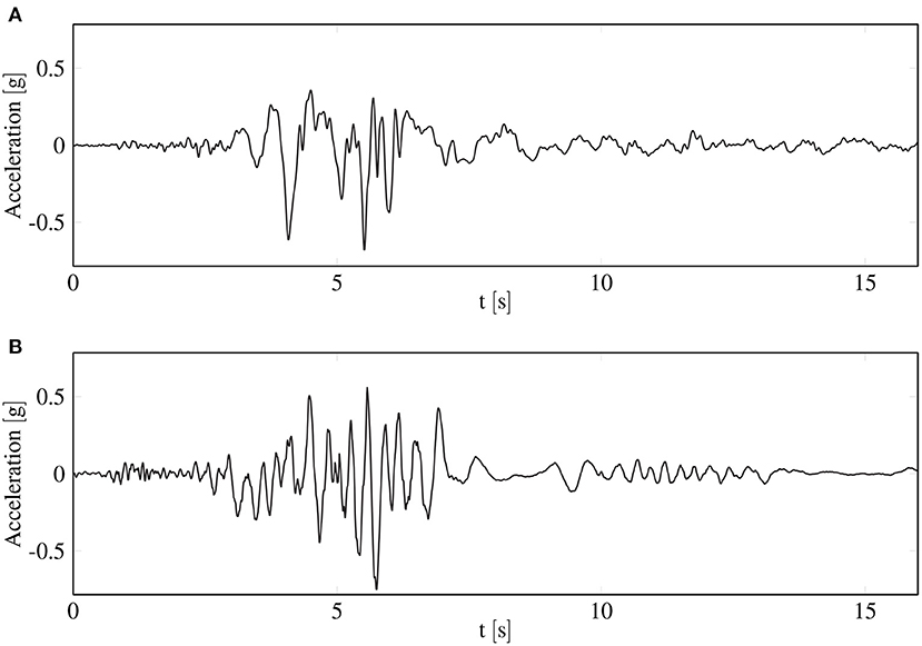
Figure 3. Ground acceleration time histories; (A) real acceleration record measured in Kobe (2016) as the benchmark earthquake; (B) artificially generated earthquake that inherits the properties from the benchmark earthquake.

Theoretically, the procedure is straightforward, as shown in Figure 4. One creates a set of ground excitation time histories ${S}$ based on which the response set ${R}$ is evaluated. Considering the limit state function g(x), every response function leads then to its corresponding indicator function value ${I}$:

$\begin{array}{l}{S}=\text{<}{\ddot{x}}_g^{(1)},\cdots ,{\ddot{x}}_g^{(m)}>\text{→ }{R}<x^{(1)}(t),\cdots ,\\ x^{(m)}(t)>\text{→ }{L}<I_g(x^{(1)}),\cdots ,I_g(x^{(m)})>& (15)\end{array}$

The evaluation of the response set ${R}$ is realized by numeric integration. In this paper, the Newmark method is used to evaluate the response function sample-by-sample (Bamer et al., 2021). However, due to relation (9), the number of samples m must be chosen disproportionately high to obtain a reliable response statistics for small probabilities of structural failure. Therefore, a realization of the crude Monte Carlo method becomes unfeasible if the system is high-dimensional and complex. In order to reliably estimate small probabilities of structural failure, we propose a strategy where a neural network is trained to learn the response behavior using a smaller training sample subset ${{S}}_T\subset {S}$, as shown in the bottom plot of Figure 4. Subsequently, the neural network can predict the full response and indicator sample sets, ${R}$ and ${I}$. One significantly benefits from the superior computational efficiency of the neural network meta-model, as it practically constitutes a series of subsequent multiplications. This strategy has one downside: the occurrence of extreme events in the sample subset ${{S}}_T$ is unlikely if the number of training subset samples is considerably smaller than the number of total samples. Neural networks will then not accurately predict the most relevant extreme events for a reliable estimation of structural failure. One measure to avoid this problem is to significantly increase the number of training subset samples, which would significantly decrease the numerical efficiency of the proposed strategy. Therefore, we pursue a different approach: we extend the training sample subset ${{S}}_T$ by introducing an additional random parameter α for the extracted intensity ẍ_r, presented in Equation (10). The extension is written as:

$\begin{array}{ll}\widehat{e}(t)={\displaystyle {\int }_{t-\frac{t_w}{2}}^{t+\frac{t_w}{2}}{\left(\alpha {\ddot{x}}_r\right)}^2}\text{d}t.& (16)\end{array}$

As shown later in the results, a unified distribution for α between 0.8 and 1.5 is a good choice for the problems in this paper. Using this extension allows us to train the neural network with a significantly higher portion of extreme events in the tail end of the distribution. The neural network is then later able to predict such relevant extreme events accurately. Instead of using a few hand-designed intensity parameters (Morfidis and Kostinakis, 2018), we use the whole excitation history as input for the neural network, as shown at the left side of Figure 5. As a result, any loss of information that could influence the structural response is avoided. In this paper, the output quantity of interest is chosen as the peak story drift ratio (PSDR) of the ground floor. However, if necessary, one can adopt the output quantity of interest. A convolutional neural network architecture is chosen for the enhanced Monte Carlo simulation method. The convolutional layers allow for automatic extraction of the time-dependent relevant patterns of the excitation time input and a breakdown of the time history information to flattened characterization parameters (see Figure 5). The subsequent fully-connected layers lead then to one output quantity of interest—the PSDR.

FIGURE 4

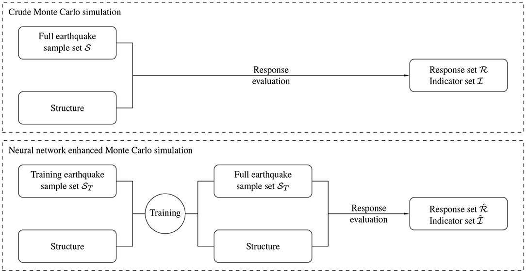
Figure 4. (Top) Crude Monte Carlo simulation workflow; (Bottom) Machine-learning-enhanced Monte Carlo simulation workflow.

FIGURE 5

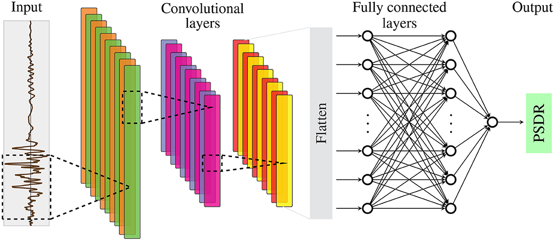
Figure 5. Convolutional neural network architecture for the enhanced Monte Carlo simulation method.

3. Numerical Results

The numerical demonstration of the new strategies is presented on a three-story two-bay frame structure subjected to the set of ground motions, as depicted in Figure 6. One ground motion sample is presented in Figure 6A and the structure is presented in Figure 6B. For the columns, beam elements with a squared hollow cross section (0.3 × 0.3 m, thickness 0.03 m) are chosen. For the beams, beam elements with a rectangular cross section (0.3 × 0.4 m, thickness 0.03 m) are chosen. Every column and beam is discretized by four fiber beam elements leading to a total number of 188 degrees of freedom (Bamer and Bucher, 2012; Bamer and Markert, 2017; Bamer et al., 2017). An elastoplastic material law with kinematic hardening is considered using the following material parameters: initial Young's modulus …2.1 × 10¹¹ N m⁻², hardening stiffness …2.1 × 10¹⁰ N m⁻², yielding stiffness …2.4 × 10⁸ N m⁻², density …7.850 kg m-3. Additionally, point masses of a value of 5.000 kg are added to every finite element node belonging to the beams of the frame structure in order to roughly consider the structural setting. We used our python and C++ based in-house tool to perform the numerical calculations.

FIGURE 6

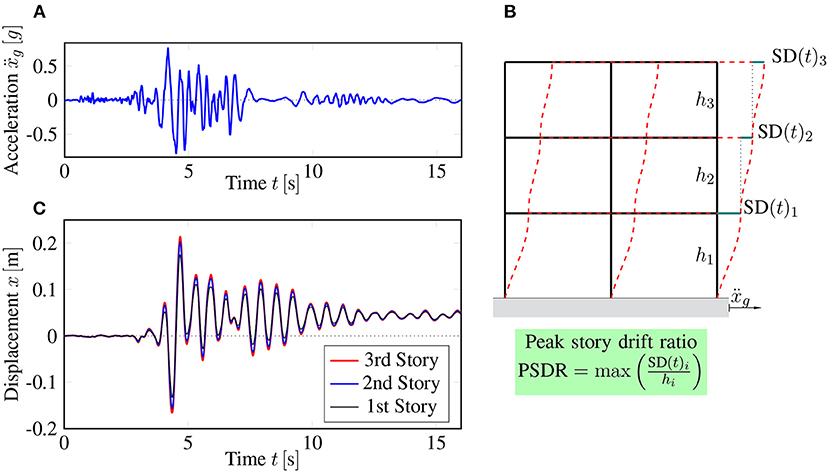
Figure 6. Structural response of a frame structure subjected to ground excitation; (A) time history of one artificially generated earthquake; (B) illustrative frame structure used for the numerical demonstration and visualization of the story drifts (SD); (C) displacement time history of the left corner of every story of the frame structure.

Using the Newmark algorithm for numeric integration, the response of the structure to the generated ground excitation (Figure 6A) is evaluated. The absolute displacement of the left corners of all three stories is depicted in Figure 6C, based on which the PSDR is extracted. One can see that the structure experiences plastic deformation due to this sample excitation, as a plastic drift-off remains after the whole integration time period. We confirmed the level of plasticity by observing the material hystereses on the Gauss-Integration point level. Plasticity mainly occurs around the frame corners of the first floors. For this example, the major displacement always occurs on the first floor, leading to the decision to take the PSDR of the first floor as the design quantity of interest.

We performed a rigorous hyperparameter search to find a neural network setup that leads to predictions of a high level of accuracy. In doing so, we found that an optimum architecture is dependent on the number of samples. If the chosen neural network architecture is chosen complex enough to extract all relevant features, a larger number of samples leads to higher accuracy of the neural network predictions. Concerning the efficiency of the proposed approach, we decided to keep the number of samples small. Therefore, the convolutional neural network architecture can also be kept simple to extract only the most relevant features. The chosen neural network architecture receives the sample excitation time history as input. Subsequently, three convolutional layers are implemented, followed by two fully connected layers, which lead to the PSDR prediction. Each convolutional layer consists of eight filters. As a result, a kernel size of 32 and a stride size of 3 have been found useful for the first convolutional layer. Regarding the second convolutional layer, the kernel size reduces to 16 with a stride size of 2. The last convolutional layer has a kernel size of 8 and a stride size of 1. After each convolutional stage, max-pooling summarizes the outputs using a pooling size of 2 and the same stride size. After passing the filters of the last convolutional layer, the outputs are averaged before the values are flattened and forwarded to the fully connected layers. The two fully connected layers consist of ten neurons each. The rectified linear activation function is applied to the convolutional stages and the fully connected layers. This architecture has shown the best accuracy if the number of samples within the sample subset of ${{S}}_{{T}}$ is 5 × 10³. Using the standard training strategy, the mean absolute error of a validation set using 10³ samples shrinks down to 1.9 × 10⁻³ after 200 epochs of training. Using the extended set for the training procedure, the mean absolute error after 200 training epochs is slightly higher with a value of 2.1 × 10⁻³. During the hyperparameter search, the number of convolutional layers was varied between one and six using up to 32 filters with kernel sizes between 3 and 64. Furthermore, the pooling sizes within the convolutional layers were varied, and both previously presented pooling functions were applied. A more extensive hyperparameter search might result in better prediction accuracy of the neural network, with high probability, if using an increased number of training samples. However, this convolutional neural network architecture can predict the PSDR accurately enough for this study. We used the Python-based library TensorFlow to implement the neural network meta-model.

The Monte Carlo simulation results are depicted in Figure 7. Within the subplots of this figure, the crude Monte Carlo simulation using 10⁵ samples is depicted by the gray dotted lines, the enhanced Monte Carlo simulation is depicted as the red lines, and the green lines depict the extended enhanced Monte Carlo simulation. We performed the numerical example on a computer with an Intel Xeon E5-2643 processor running at 3.3 GHz. The operating system is Linux Ubuntu 16.04 with 60 GB of working memory available, which is by no means required for the simulation. For the example in this paper, the crude Monte Carlo simulation requires a calculation time of ~1 week, while the prediction procedure of the two neural network-enhanced strategies requires only a few seconds. However, to provide a fair speed-up measure, one must consider evaluating the training sample set, the hyperparameter fitting, and the training procedure. Considering those factors, we chose a fair speed-up measure for the new strategies by dividing the number of full samples by the number of training samples. The numerical demonstration results in a value of 10⁵ samples for the full set and over 5 × 10³ samples for the training set, which results in a speed-up factor of 20.

FIGURE 7

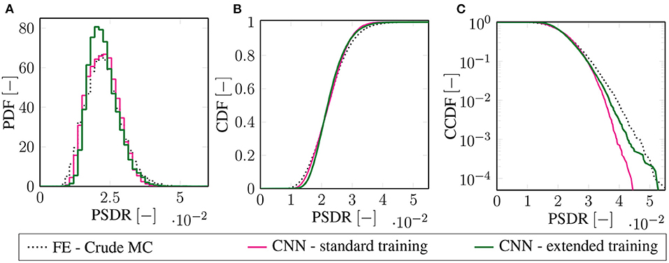
Figure 7. (A) Probability density function (PDF), (B) cumulative distribution function (CDF), and (C) logarithmic plot of the complementary cumulative distribution function applying the crude Monte Carlo method (black, dotted line), the neural network-enhanced Monte Carlo method using the standard training strategy (red line), and the neural network-enhanced Monte Carlo method using the extended training strategy (green line).

Figure 7A presents the probability density function (PDF) in terms of a histogram over the displacement intervals. At first sight, one can see that the enhanced Monte Carlo simulation method using the extended scheme is not as accurate as the enhanced Monte Carlo using the standard training scheme. Also, regarding the cumulative distribution function (CDF) prediction, shown in Figure 7B, the enhanced Monte Carlo simulation scheme using the standard training algorithm seems to be more accurate than the enhanced Monte Carlo method using the extended training scheme. This is not surprising as the neural network is better trained around the mean using standard sample subset ${{S}}_T$ then using the extended subset ${\widehat{{S}}}_T$. However, accuracy around the mean is not that relevant in structural engineering design, as, for obvious reasons, we want structural failure to happen very rarely. Therefore, we present the tail end of the complementary cumulative distribution function (CCDF) in Figure 7C, which shows the occurrence of exceeding a certain PSDR in a logarithmic plot. Here, the clear advantage of the enhanced Monte Carlo simulation using an extended sample subset becomes clear, as it outperforms the standard, enhanced Monte Carlo simulation in the crucial region around the tail end of the distribution. Evaluating the probability of exceedance for a PSDR over 3.5 × 10⁻² m results in a reliable approximation using the extended neural network enhanced strategy, while the neural network enhanced method using the standard training becomes gradually more inaccurate until the method entirely fails for predicting the probability of a PSDR exceeding a value of 4.2 × 10⁻² m.

4. Conclusion

In this paper, we proposed a new Monte Carlo simulation method enhanced by a convolutional neural network. Using a non-linear Kanai-Tajimi filter, site-dependent ground conditions were taken into account. Two convolutional neural network-enhanced strategies were proposed. The first strategy uses a standard training procedure by considering samples from the full excitation sample set. The second strategy uses a sample set with increased variance regarding intensity to train the neural network more around the tail end of the distribution. In the presented numerical example, the PSDR is the output quantity. However, the proposed strategy can be adapted to predict other output features. The investigation on a more sophisticated damage prediction using multiple output quantities is of high interest for future research.

We have shown that both strategies reveal outstanding efficiency when compared to the crude Monte Carlo simulation. Structural design that incorporates non-linear behavior has practically not been realized using the Monte Carlo method as it was yet not possible in a feasible amount of time. However, the new strategies allow for Monte Carlo simulations in a feasible amount of time that can now be incorporated into a practical design environment. The accuracy of the convolutional neural network is dependent on the number of training samples. Accordingly, one always makes a trade-off between the accuracy of the predictions and the computing time for evaluating the training samples.

The two types of convolutional neural network enhanced Monte Carlo simulation strategies have different advantages and disadvantages. The first type of the new method applying the standard training strategy shows a high accuracy around the mean of the distribution. One can conclude that they will be more useful for estimations of the response regarding structural serviceability. The second type of the new method applying the extended training strategy reveals to be rather more inaccurate around the mean of the distribution than the first type. However, it reveals an outstanding accuracy around the tail end of the distribution, where the first method fails. It is, therefore, highly appropriate to be applied to practical engineering procedures that involve the design of structures considering the low target probability of failure that is, especially, required for engineering structures in an urban built environment.

Data Availability Statement

The original contributions presented in the study are included in the article/supplementary material, further inquiries can be directed to the corresponding author/s.

Author Contributions

FB and DT developed the new method, performed the numerical simulations, and wrote the manuscript. MS and BM reviewed the manuscript and supervised the research project. All authors contributed to the article and approved the submitted version.

Conflict of Interest

The authors declare that the research was conducted in the absence of any commercial or financial relationships that could be construed as a potential conflict of interest.

References

Bamer, F., Amiri, A., and Bucher, C. (2017). A new model order reduction strategy adapted to nonlinear problems in earthquake engineering. Earthq. Eng. Struct. Dyn. 46, 537–559. doi: 10.1002/eqe.2802

CrossRef Full Text | Google Scholar

Bamer, F., and Bucher, C. (2012). Application of the proper orthogonal decomposition for linear and nonlinear structures under transient excitations. Acta Mech. 223, 2549–2563. doi: 10.1007/s00707-012-0726-9

CrossRef Full Text | Google Scholar

Bamer, F., and Markert, B. (2017). An efficient response identification strategy for nonlinear structures subject to nonstationary generated seismic excitations. Mech. Based Des. Struct. Mach. 45, 313–330. doi: 10.1080/15397734.2017.1317269

CrossRef Full Text | Google Scholar

Bamer, F., Shi, J., and Markert, B. (2018). Efficient solution of the multiple seismic pounding problem using hierarchical substructure techniques. Comput. Mech. 62, 761–782. doi: 10.1007/s00466-017-1525-x

CrossRef Full Text | Google Scholar

Bamer, F., Shirafkan, N., Xiaodan, C., Oueslati, A., Stoffel, M., de Saxcé, G., et al. (2021). A newmark space-time formulation in structural dynamics. Comput. Mech. 1–19. doi: 10.1007/s00466-021-01989-4

CrossRef Full Text | Google Scholar

Bucher, C. (2009). Computational Analysis of Randomness in Structural Mechanics, Vol. 3. London: Tayler & Francis.

Google Scholar

Der Kiureghian, A. (1996). Structural reliability methods for seismic safety assessment: a review. Eng. Struct. 18, 412–424. doi: 10.1016/0141-0296(95)00005-4

CrossRef Full Text | Google Scholar

Fujimura, K., and Der Kiureghian, A. (2007). Tail-equivalent linearization method for nonlinear random vibration. Probabil. Eng. Mech. 22, 63–76. doi: 10.1016/j.probengmech.2006.08.001

PubMed Abstract | CrossRef Full Text | Google Scholar

Goodfellow, I. J., Bengio, Y., and Courville, A. (2016). Deep Learning. Cambridge, MA: MIT Press. Available online at: http://www.deeplearningbook.org

Google Scholar

Hurtado, J., and Barbat, H. (1998). Monte Carlo techniques in computational stochastic mechanics. Archiv. Comput. Methods Eng. 5, 3–30. doi: 10.1007/BF02736747

PubMed Abstract | CrossRef Full Text | Google Scholar

Kobe (2016). Kobe Takarzuka Earthquake Measurement 1995–01-16 20:46:52 UTC. Center for Engineering Strong Motion Data. Virtual Data Center. Available online at: www.strongmotioncenter.org/

Koeppe, A., Bamer, F., and Markert, B. (2019). An efficient Monte Carlo strategy for elasto-plastic structures based on recurrent neural networks. Acta Mech. 230, 3279–3293. doi: 10.1007/s00707-019-02436-5

CrossRef Full Text | Google Scholar

Koeppe, A., Bamer, F., and Markert, B. (2020). An intelligent nonlinear meta element for elastoplastic continua: deep learning using a new time-distributed residual U-Net architecture. Comput. Methods Appl. Mech. Eng. 366:113088. doi: 10.1016/j.cma.2020.113088

CrossRef Full Text | Google Scholar

Kruse, R., Borgelt, C., Braune, C., Klawonn, F., Moewes, C., and Steinbrecher, M. (2015). Computational Intelligence, Eine Methodische Einführung in Künstliche Neuronale Netze, Evolutionäre Algorithmen, Fuzzy-Systeme und Bayes-Netze. Wiesbaden: Springer Vieweg.

Google Scholar

Liao, W., Chen, X., Lu, X., Huang, Y., and Tian, Y. (2021). Deep transfer learning and time-frequency characteristics-based identification method for structural seismic response. Front. Built Environ. 7:10. doi: 10.3389/fbuil.2021.627058

CrossRef Full Text | Google Scholar

Lu, X., Liao, W., Huang, W., Xu, Y., and Chen, X. (2020). An improved linear quadratic regulator control method through convolutional neural network–based vibration identification. J. Vib. Control 27:107754632093375. doi: 10.1177/1077546320933756

CrossRef Full Text | Google Scholar

Lu, X., Xu, Y., Tian, Y., Cetiner, B., and Taciroglu, E. (2021). A deep learning approach to rapid regional post-event seismic damage assessment using time–frequency distributions of ground motions. Earthq. Eng. Struct. Dyn. 50, 1612–1627. doi: 10.1002/eqe.3415

CrossRef Full Text | Google Scholar

Morfidis, K., and Kostinakis, K. (2018). Approaches to the rapid seismic damage prediction of R/C buildings using artificial neural networks. Eng. Struct. 165, 120–141. doi: 10.1016/j.engstruct.2018.03.028

CrossRef Full Text | Google Scholar

Roberts, J., and Spanos, P. (1990). Random Vibration and Statistical Linearization. New York, NY: John Wiley & Sons.

Google Scholar

Stoffel, M., Bamer, F., and Markert, B. (2018). Artificial neural networks and intelligent finite elements in non-linear structural mechanics. Thin Walled Struct. 131, 102–106. doi: 10.1016/j.tws.2018.06.035

CrossRef Full Text | Google Scholar

Stoffel, M., Bamer, F., and Markert, B. (2019). Neural network based constitutive modeling of nonlinear viscoplastic structural response. Mech. Res. Commun. 95, 85–88. doi: 10.1016/j.mechrescom.2019.01.004

CrossRef Full Text | Google Scholar

Stoffel, M., Bamer, F., and Markert, B. (2020a). Deep convolutional neural networks in structural dynamics under consideration of viscoplastic material behaviour. Mech. Res. Commun. 108:103565. doi: 10.1016/j.mechrescom.2020.103565

CrossRef Full Text | Google Scholar

Stoffel, M., Gulakala, R., Bamer, F., and Markert, B. (2020b). Artificial neural networks in structural dynamics: a new modular radial basis function approach vs. convolutional and feedforward topologies. Comput. Methods Appl. Mech. Eng. 364:112989. doi: 10.1016/j.cma.2020.112989

CrossRef Full Text | Google Scholar

Sun, H., Burton, H. V., and Huang, H. (2021). Machine learning applications for building structural design and performance assessment: state-of-the-art review. J. Build. Eng. 33:101816. doi: 10.1016/j.jobe.2020.101816

CrossRef Full Text | Google Scholar

Thaler, D., Bamer, F., and Markert, B. (2021a). A machine learning enhanced structural response prediction strategy due to seismic excitation. PAMM 20:e202000294. doi: 10.1002/pamm.202000294

CrossRef Full Text | Google Scholar

Thaler, D., Stoffel, M., Markert, B., and Bamer, F. (2021b). Machine learning enhanced tail end prediction of structural response statistics in earthquake engineering. Earthq. Eng. Struct. Dyn. eqe3432. doi: 10.1002/eqe.3432

CrossRef Full Text | Google Scholar

Zhang, R., Liu, Y., and Sun, H. (2020). Physics-guided convolutional neural network (PHYCNN) for data-driven seismic response modeling. Eng. Struct. 215:110704. doi: 10.1016/j.engstruct.2020.110704

CrossRef Full Text | Google Scholar