Applicability of Convolutional Neural Networks for Calibration of Nonlinear Dynamic Models of Structures

1 Introduction

This study examines the applicability of a convolutional neural network (CNN)-based machine learning (ML) framework for calibrating the parameters of analytical models of nonlinear mechanical/structural systems with limited experimental data. Large-scale experiments on structural elements, such as bridge columns, are cost prohibitive. Traditionally, analytical models are used to supplement experimental data and investigate effects of a variety of design variables. However, complex nonlinear models contain a large number of parameters that require approximation. This is conventionally done through basic statistical or data-fitting methods to achieve a desired performance, such as an accurate prediction of load-displacement relationships (Willard et al., 2020). The conventional approaches, however, may fail to capture complex interactions of modeling parameters or lead to subjective outcomes when analytical models involve a large number of parameters requiring calibration. In this work, the seismic response of a composite bridge column is used as the case study for the evaluation of a transfer learning framework, where an ML model is trained with a large synthetic dataset and then used to obtain calibrated parameters for one or a few sets of experimental data. The composite column consisted in this study is a fiber-reinforced polymer (FRP) tube with a reinforced concrete (RC) core. A large-scale model of this column was previously tested at the University of Nevada, Reno on a shake table (Zaghi et al., 2012). An analytical model of the column capturing material plasticity, non-linear composite action of the tube and the concrete core, base rotations, and inelastic shear deformation was developed in the OpenSees structural modeling platform. The large number of modeling variables and their complex nonlinear interactions in a such model may lead traditional calibration methods to have subjective outcomes. Thus, ML, in particular a CNN, is used to calibrate the parameters of the analytical model. The network is trained using the lateral load, axial load, and displacement time histories as the input variables and the analytical modeling parameters as the output variables. The trained network is then used to obtain the calibrated parameters for the experimental data.

ML techniques have been used successfully to identify mechanical characteristics of different types of materials under complex loading conditions, including variable temperatures, high-rate loads, and triaxial stresses (Tang, 2010; Gandomi et al., 2012; Rafiei et al., 2016; Huang and Burton, 2019; Kang et al., 2021). ML techniques, such as artificial neural networks and gene expression programming, have also been used to identify strength of reinforced concrete columns and walls using experimental data (Ilkhani et al., 2019; Murad et al., 2020; Murad, 2021; Naderpour et al., 2022). However, ML techniques require large datasets for the successful training of the model, which are expensive to obtain experimentally. Thus, these studies often rely on previously conducted experiments, which can limit their applicability to well-established materials with ample experimental data, such as reinforced concrete. However, the recent enhancements in computation power have enabled development of large datasets using analytical simulations. These large datasets have promoted the application of deep learning methods for complex nonlinear materials (Liu et al., 2019; Chen et al., 2021), such as the damage progression of composites (Yan et al., 2020). However, the applicability of ML to the calibration of nonlinear mechanical/structural systems under complex loading has not been fully explored, which the framework proposed in this study aims to address. Complex structural systems often contain different types of material and various sources of nonlinearity in addition to the material plasticity. Traditional ML techniques, such as shallow artificial neural networks, often require pre-processing steps to select optimal features from raw data. Deep neural networks, such as CNNs, offer the advantage of extracting inherent features in high-dimensional spaces directly from the data (Sadoughi and Hu, 2019; Kiranyaz et al., 2021). This will enable “matching” the entire shape of the hysteresis curve rather than a few engineering parameters or the backbone curve. A significant portion of the information about the nonlinear response of a complex system is encoded in the hysteresis curves. Thus, a deep learning model that is capable of learning complex visual features will offer promise for the successful calibration of difficult parameters of nonlinear analytical models, and ultimately will enhance the accuracy of simulations.

CNNs are traditionally used for two-dimensional (2D) signals, such as images or videos. The convolutional layers apply kernels over regions of the input to extract complex visual features of an image at different scales, which are presented as feature maps. CNNs capture the spatial relationship between features on an image. Alternatively, one-dimensional (1D) CNNs have been used for signal processing applications, such as structural health monitoring, high-power engine fault monitoring, and structural damage detection by extracting complex features of time-series data (i.e., signals) (Kiranyaz et al., 2015; Avci et al., 2017; Chen and Wang, 2019; Yu et al., 2019; Kiranyaz et al., 2021). In 1D CNNs, the kernel is applied along the time-series in one direction, extracting features from the adjacent timesteps. Researchers have also proposed reshaping the signals into 2D arrays to take advantage of 2D kernels, which use the adjacent rows and columns for feature extraction (Hoang and Kang, 2017; Zhang et al., 2017). In addition to reshaped time-domain signals, researchers have proposed using time-frequency representations to take advantage of the 2D feature extraction of CNNs. Time-frequency transformations let us illustrate the temporal variations of frequency features of a signal, resulting in a 2D matrix that can be processed as an image data. In engineering applications, this is an efficient and conventional approach for analyzing and extracting temporal variations of the features from nonstationary time-series data (Spanos et al., 2007; Nagarajaiah and Basu, 2009; Balli and Palaniappan, 2010; Kong et al., 2017; Kim et al., 2017; Silik et al., 2021). The most common representations are spectrograms and scalograms, which have recently been used with CNNs to extract deep features of signals that typically require manual feature extraction performed by an expert (Xu et al., 2018; Khan et al., 2019; Khare and Bajaj, 2020; Pham et al., 2020; Zhang et al., 2020). While previous studies have shown image representations of engineering signals are suitable for training CNNs, the applications are typically limited to classification tasks or damage identification. Thus, the ability to model calibration of a system with different materials and many sources of nonlinearity has not been fully explored. The framework. To address this, the applicability of the framework to multiple image-based representations of the signals was investigated to establish the suitability of different representation methods to parameter calibration tasks.

This work proposes a novel deep learning framework for calibrating the parameters of analytical models representing complex nonlinear mechanical/structural systems when experimental data is limited (e.g., results from one or two experiments.) The framework was evaluated by calibrating the parameters of an analytical model representing the shake table response of a composite structural column. The developed analytical model included new modeling approaches for aspects of the composite column that were neglected in previous studies, such as FRP-to-concrete core bond, nonlinear shear deformations, and bond-slip, in an effort to improve the accuracy capturing the lateral force and dissipated energy. The analytical model representing the system was used to generate a large-enough synthetic dataset given different permutations of the parameters requiring calibration. A CNN was trained using the lateral load, axial load, and displacement time histories as the input variables and the model parameters as the output variables. Using a synthetic dataset allowed deep learning techniques to be used without sufficient experimental data and allowed the learning to be centered on the underlying relationships and interactions of these parameters. The synthetic dataset (i.e., analytical results) complied with the physical phenomena, such as constitutive relationships, equilibrium, and energy and momentum conservation, is captured by the analytical model. Thus, the deep learning model learns these concepts from the analytical results rather than a large dataset of physical experiments. Additionally, as the framework uses a dataset of only model inputs and outputs, it can be adapted to analytical models of various complexities with little to no change to its structure. The applicability of the framework to multiple image-based representations of the signals was investigated to establish the suitability of different representation methods to parameter calibration tasks. This included presenting the time histories in the time-domain and time-frequency domain when training a CNN. The time-domain input was used to train two CNNs to compare 1D and 2D convolution kernels. Two time-frequency domain inputs, spectrograms and scalograms, were used. The performance of the trained networks in capturing peak lateral force, residual displacement, and hysteresis energy dissipation in addition to the individual model parameters were used for evaluation. Finally, the trained networks were prompted with the experimental data from the shake table test to obtain the analytical model parameters for the composite column system.

The predicted parameters from the proposed framework captured the experimental response with higher accuracy across the time-series than the previously proposed analytical models for the composite column system. This accuracy demonstrates for the first time that image representations of engineering signals are suitable for training CNNs for model calibration of nonlinear structural systems. The various sources nonlinearity and damping as well as the large number of parameters, allowed benefits of both the time-series and time-frequency presentations to be realized. For this application, the time-series networks had superior performance. The results of the proposed framework also demonstrated that a synthetic dataset can be sufficient for training a CNN that will subsequently be used with experimental data without requiring additional training. This indicates further potential for transfer learning applications using the framework, where it can be retrained with small datasets to performance a related task, such as calibration of a different structural system.

2 Methods and Approach

An analytical model was developed to simulate the shake table response of a composite bridge column with an FRP tube and RC core that was previously tested at the University of Nevada, Reno (Zaghi et al., 2012). These composite columns were developed as a durable alternative to conventional RC columns. While they have shown superior structural performance to RC columns, the exterior composite tube and its interaction with the concrete core introduce additional modeling complexities that lack established modeling strategies. Additionally, even well-established materials, such as steel and concrete, have properties that vary due to strain-rate effects or parameters characterizing their constitutive relationships that are not easily identifiable from mechanical tests (Kulkarni and Shah, 1998; Zadeh and Saiidi, 2007; Carreño et al., 2020). As such, parameter calibration for the shake table testing of the composite column provided both a relevant and challenging case study for the evaluation of the proposed framework. A total of 25 model parameters requiring calibration were selected from the analytical model. These parameters included the constitutive behavior of the concrete core, steel reinforcement, and exterior composite tube, as well as interactions between the concrete core and the composite tube, global and local damping coefficients, base fixity, and nonlinear shear deformations. The measured displacement and axial load time histories from the shake table test were used as the input signals in the OpenSees model, which then generated the lateral load time history. A synthetic dataset was generated by varying the 25 model parameters. A supervised learning framework was used to learn the relationships between the model parameters as the target vector and displacement, axial load, and lateral load time histories as the input data. The experimental test, composite column system, and analytical model are detailed in the following sections.

2.1 Experimental Test and Composite Column System

The shake table test was performed on a 370-mm diameter by 1511-mm long concrete-filled FRP tube (CFFT) column system (Zaghi et al., 2012). The experimental test setup is shown in Figure 1A. The CFFT column had an FRP tube with glass fibers oriented at ±55°, an inner diameter of 355.6 mm, and a thickness of 7 mm. The unconfined concrete had a compressive strength of 47.4 MPa on the test day. The steel reinforcement included 8-#13 longitudinal bars (Figure 1B). The FRP tube provided confinement for the concrete core and functioned as transverse reinforcement for shear resistance.

FIGURE 1

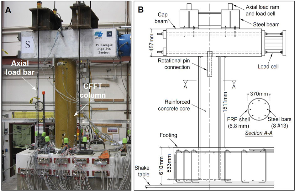
FIGURE 1. (A) Experimental test setup showing CFFT column on the shake table prior to testing and (B) structural detail including components of the test setup and internal steel reinforcement.

The input motion for the shake table test was a ground acceleration recorded during the 1994 Northridge, CA earthquake (Hauksson et al., 1995). The input motion was applied in seven progressive runs, with acceleration scale factors increasing from 0.1 to 1.9. An axial load of 222 kN was applied on the column using four high-strength rods and measured by two load cells during the tests. The axial load fluctuated between 85 and 390 kN during the tests due to the small vertical displacement of the cap beam causing the axial load rods to stretch. Additional details regarding the CFFT column system, the construction of the specimen, and the experimental setup can be found in Zaghi et al. (Zaghi et al., 2012).

2.2 Analytical Model

The analytical modeling was performed in OpenSees, which is an open-source, object-oriented structural analysis framework (Mazzoni et al., 2009). The model was developed to capture the global and local responses of the CFFT column. The schematic view of the nonlinear analytical model is shown in Figure 2 along with the element types, material commands, and constitutive material models. The CFFT column was modeled using displacement-based elements with fiber cross-sections representing the longitudinal steel bars, FRP-confined concrete core, and longitudinal behavior of the FRP tube. The lateral displacement, δ(t), and axial load, P(t), time histories recorded during the experimental shake table test were used as input signals for the analytical model. Figure 2 shows these input functions during Runs 4 through 7. The general analytical model details are discussed below, with a focus on the parameters requiring calibration.

FIGURE 2

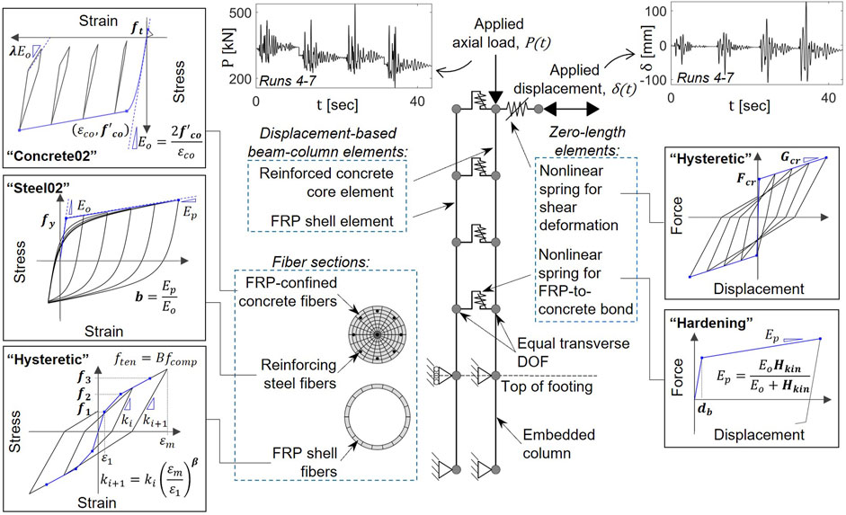
FIGURE 2. Schematic view of the nonlinear analytical model of a CFFT column modeled using OpenSees. Plots of the applied axial load and displacement time histories and constitutive material behavior are presented. The material commands are identified along with the general shape of the hysteresis curves. The parameters included for calibration are shown in boldface.

The FRP-confined concrete core behavior was defined using the model proposed by Teng et al. (Teng et al., 2009) and assigned to the uniaxial material “Concrete02”. The steel reinforcement was modeled using the uniaxial material “Steel02”, defined by the Guiffre-Menegotto-Pinto model with isotropic strain hardening (Filippou et al., 1983). The longitudinal behavior of the FRP tube was modeled using the uniaxial material “Hysteretic” in combination with the uniaxial material “Maxwell” to represent the viscoelastic response of the composite tube. The initial envelope curve for the FRP tube was based on previous experimental and analytical models from Shao et al. (Shao, 2003) and Zaghi et al. (Zaghi et al., 2012) for filament wound FRP tubes with fibers at ±55°. The constitutive material models are provided in Figure 2. The reinforced concrete core and the FRP tube were modeled using separate elements, as shown in Figure 2, to capture any bond slippage between the FRP tube and concrete core elements (i.e., partial composite action), which was previously observed during the shake table test (Zaghi et al., 2012). To capture this behavior, the cantilever part of each element was discretized into four sections and connected with nonlinear shear and rotational springs using “ZeroLength” elements, with the constitutive behaviors defined in Figure 2. The preliminary break point was estimated using the strains measured on the FRP tube and steel bars during the experiment (Zaghi, 2009). Multi-point constraints were defined between the nodes for the FRP tube and the concrete core in the transverse direction (Figure 2). The lateral displacement and axial load were applied to the top node of the concrete core element. The initial shear stiffness of the CFFT column was defined using the uncracked concrete section properties. The post-cracking shear stiffness was defined by the cracked concrete section and FRP tube properties. The embedded portion of the CFFT column was modeled using an embedded element to explicitly capture the effects of base rotation. The effect of potential construction misalignment was captured by two zero-length, compression-only springs at the top of the column with a gap for initial surface asymmetry. Mass- and stiffness-proportional damping were defined using the “rayleigh” command.

2.2.1 Target Variables for the Convolutional Neural Network

Twenty-five analytical model parameters, shown in Table 1, that required calibration were defined as target variables when training the CNN. These include material properties for the individual components of the CFFT column, such as the FRP tube, reinforced-concrete core, and steel reinforcement. Parameters defining system-level interactions were also included, such as the nonlinear shear behavior, FRP-to-concrete bond behavior, and construction misalignment. Additionally, the critical-damping ratio and frequency were included, which define the mass- and stiffness-proportional damping coefficients (Wilson, 2004). The parameter details are included in Table 1. The schematic constitutive material behaviors are presented in Figure 2 and include definitions of the calibration parameters, which are shown in bold. The ranges of the parameters were selected to encompass the expected values estimated through material testing, specified material properties, and engineering judgment (Wilson, 2004; Burgueño and Bhide, 2006; Zhu et al., 2006; Teng et al., 2009; Systems, 2012; Zaghi et al., 2012).

TABLE 1

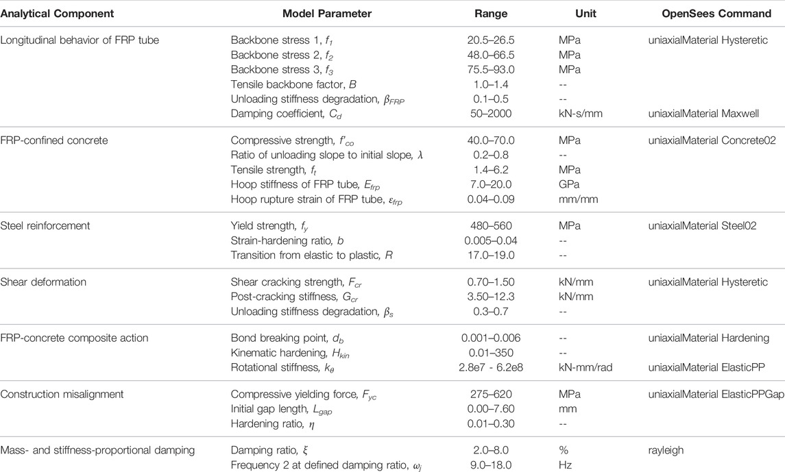
TABLE 1. Details of model parameters to be calibrated by the CNN, including the modeling component, interval of input values, and OpenSees commands.

3 Framework for Analytical Model Parameter Calibration

The following sections discuss the training data generation, data preparation, and network architectures for the different input representation methods. Next, the evaluation metrics and process for obtaining the calibrated parameters for the composite column system are detailed. The complete workflow of the proposed framework is shown in Figure 3. In the proposed workflow, the analytical model representing the composite column is used to generate a synthetic dataset for training a CNN. The input to the analytical models includes the model parameters (Table 1) as well as the displacement and axial load time histories measured during the shake table test. The lateral load responses from the analytical model are combined with the displacement and axial load and used as the input data when training the CNN. The corresponding model parameters are the target outputs. After training and evaluating with the synthetic dataset, the CNN is prompted with the experimental data for the composite column and the calibrated model parameters are obtained.

FIGURE 3

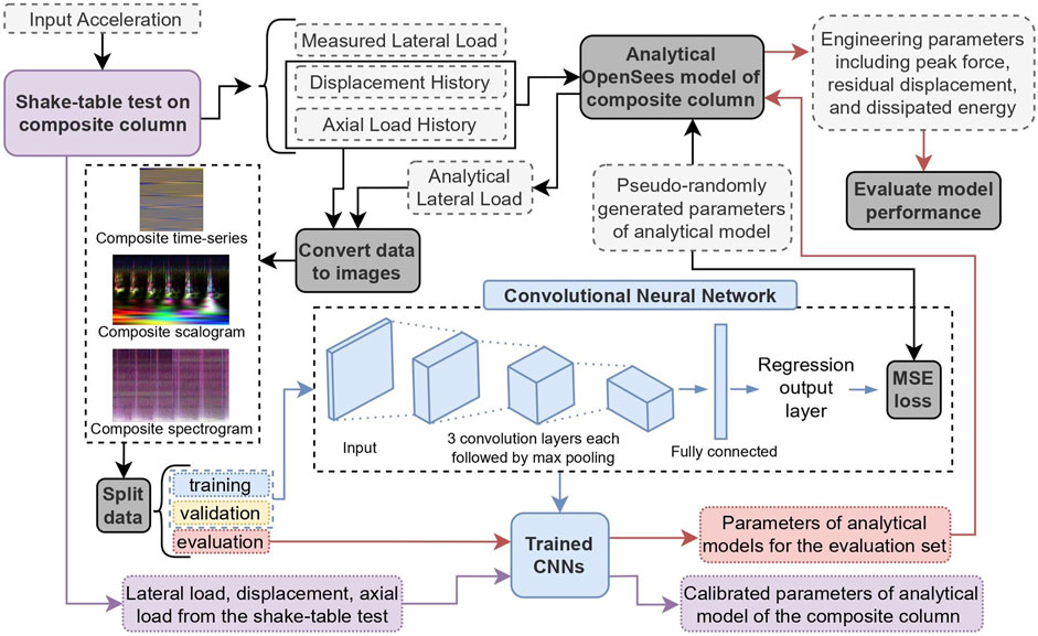
FIGURE 3. Complete workflow of the proposed framework, including generating the training data, evaluating the trained networks using the engineering metrics, and obtaining calibrated parameters for the composite column system.

3.1 Training Data

The analytical model previously introduced was used to generate the synthetic dataset for training the CNNs. The model parameters to be calibrated were defined using a quasi-random number generator (QRNG) within the bounds shown in Table 1. QRNGs minimize discrepancy between generated points to fill the multi-dimensional space in a uniform manner (Skublska-Rafajłowicz and Rafajłowicz, 2012). This results in a comprehensive representation of the 25 parameters and their effect on the analytical lateral load. The quasi-random number dataset was generated using the Sobol sequence (Sobol', 1967). The first 1,000 points were omitted, and the sequence was scrambled using Owen’s scrambling algorithm to reduce correlations and improve uniformity (Matoušek, 1998).

In addition to the target parameters, i.e., calibration parameters, the input displacement and axial load were varied within the synthetic dataset. This was done by adding Gaussian white noise (GWN) to the displacement and axial load time histories prior to running the analytical simulations, as a method of data augmentation and regularization to mitigate overfitting (Rochac et al., 2019). This approach also provided supplementary information on the instantaneous stiffness of the system and time-dependent behavior, such as Rayleigh damping and viscoelasticity. The magnitude of the noise added to the displacement signals varied between 0.25 and 2.5 mm. Random weighting of the two load cells measuring the axial load was applied in addition to GWN with a signal-to-noise ratio (SNR) of 30 dB. Varying the axial load was necessary to provide a comprehensive representation of the asymmetric behavior of the FRP tube and concrete core in tension and compression.

A total of 50,000 samples were generated for the synthetic dataset, where the analytical lateral load varied based on the input displacement, axial load, and model parameters. As one objective of this work is to evaluate and compare the input methods, a large dataset was used to ensure that the performance was not being meaningfully limited by the amount of training data.

3.2 Data Preparation

CNNs were developed primarily for images, which are simply 2D arrays where the cell value defines the pixel intensity. An RGB image stores the red, green, and blue pixel values in separate color channels, which can also be viewed as three different 2D arrays. As such, after converting to 2D arrays, the lateral force, displacement, and axial load signals can be stored in separate channels and used as a single input image for training a CNN. A variety of approaches for converting the signals to images have been implemented in previous studies (Kiranyaz et al., 2021). The main approaches typically fall into two categories 1) using the raw signal in the time domain or 2) transforming the signal into the time-frequency domain. In the first approach, the signal is rescaled so that the amplitude represents the pixel intensity (typically to an integer between 0 and 255). The signal can be reshaped to create an $m\times n$ array, i.e., an image. The engineering applications of this approach are for vibration and electrocardiogram signals (Kolar et al., 2020; Wang et al., 2020; Wang et al., 2021; Zare and Ayati, 2021). In the second approach, a time-frequency transformation is used to represent the signal in the time and frequency domains simultaneously, resulting in a 2D signal that is plotted as an image to visualize the signal activity. The most popular representations are spectrograms and scalograms, which are commonly used in engineering applications to extract features from signals (Spanos et al., 2007; Nagarajaiah and Basu, 2009; Balli and Palaniappan, 2010; Kong et al., 2017; Kim et al., 2017; Silik et al., 2021). Recently, these representations have been used with CNNs to automatically extract features that typically require manual methods informed by expert knowledge (Xu et al., 2018; Khan et al., 2019; Khare and Bajaj, 2020; Pham et al., 2020; Zhang et al., 2020). This work investigated training CNNs for parameter calibration using both the raw time-series signals and the transformed time-frequency representations. The time-series data was used to train two CNNs to evaluate 1D and 2D convolution kernels; these networks are referred to as TS-1D and TS-2D, respectively. Additionally, the time-frequency representations, spectrograms and scalograms, were used to train two CNNs, referred to as TF-SP and TF-SC, respectively. A summary of the input for each of the four networks is provided in Table 2 and representative inputs are shown in Figure 4. The following sections discuss generating the training dataset as well as background on the approaches.

TABLE 2

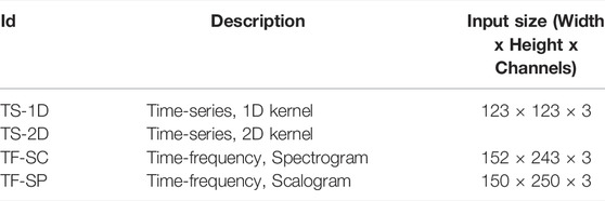
TABLE 2. Summary of inputs and trained networks.

FIGURE 4

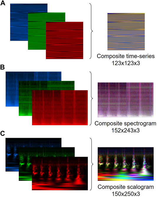
FIGURE 4. Sample composite input and corresponding lateral load, displacement, and axial load components for the (A) time-series (B) spectrogram, and (C) scalogram inputs.

3.2.1 Generating Time-Domain Training Dataset

Previous applications of this approach have typically been in 1D CNNs, where the convolution kernels extract features from the adjacent points along the time-series (Kiranyaz et al., 2021). These applications are commonly using CNNs for real-time monitoring or damage detection/localization and have limited available training data, making the computationally efficient 1D CNN advantageous. As the proposed framework uses synthetic data, sufficiently large datasets can be generated to train a 2D CNN. A 2D convolution kernel uses both the adjacent rows and columns for feature extraction, which provides information across different cycles in addition to the adjacent timesteps. This may provide a more robust feature extraction as the model parameters typically influence the response across multiple cycles.

This work reshaped the signals by wrapping the 1D arrays into 2D arrays, which can be used to train a CNN with either a 1D or 2D kernel. The lateral load, displacement, and axial load signals reshaped into a 123-by-123 matrix. The signals values were normalized to be integers between 0 and 255. Next, the normalized lateral load, displacement, and axial load signals were assigned to separate color channels within an RGB image to create a single input with dimensions of 123-by-123-by-3. A sample RGB image and the lateral load, displacement, and axial load components are shown in Figure 4A. Additional information on 1D and 2D convolution kernels is provided when presenting the CNN architectures.

3.2.2 Generating Time-Frequency Domain Training Datasets

Representing the signals in the time-frequency domain was investigated using spectrograms and scalograms, which are generated by a short-time Fourier transform (STFT) and continuous wavelet transform (CWT), respectively. Time-frequency representations provide a visualization of the signal activity and have been used to extract modal properties and detect damage in structures (Nagarajaiah and Basu, 2009; Kong et al., 2017; Silik et al., 2021). As such, these inputs may facilitate the extraction of frequency-related parameters, such as damping and stiffness. However, this is at the cost of temporal resolution as there is a limit to the degree a signal can be localized both in time and frequency, as shown by Heisenberg’s uncertainty principle (Cohen, 1995). The wavelet transform aims to mitigate the limitations due to the trade-off between time and frequency resolutions by applying a variable-size wavelet. This approach allows the time-frequency resolution to change within the scalogram, where the STFT applies a window function with a fixed length, resulting in a constant time-frequency resolution. As a result, the spectrogram is less accurate in capturing time-localized information than the scalogram, especially when the duration of events in a signal differs significantly. CWTs are computationally more complex than STFT (Bouchikhi et al., 2011); thus, slight improvements in accuracy may not warrant the application of scalograms when large datasets are required.

The spectrograms were generated using a Hanning window with a width of 120 data points and an overlap length of 50% to prevent information loss due to the Picket Fence effect (Cerna and Harvey, 2000). The magnitude of the STFT was plotted as a function of both time and frequency, shown on the y- and x-axis, respectively. The spectrograms were generated for the lateral load, displacement, and axial load signals and assigned to the red, green, and blue channels of a 2D RGB image to create a single composite image as shown in Figure 4B.

The second TF representation, scalograms, were obtained by applying a CWT, which dilates and translates the signal along the time axis using a defined wavelet. Analytic Morse wavelets were used with a shape parameter of 3 and time-bandwidth product of 60. These wavelets are symmetric in the time domain and nearly symmetric in the frequency domain while maintaining a high time/frequency concentration (Lilly and Olhede, 2008; Lilly and Olhede, 2012; Lilly, 2017). The modulus of the complex-valued wavelet coefficients obtained from the CWT were scaled by the maximum values at each frequency. The scaled wavelet coefficients were plotted as a function of frequency and time, shown on the y- and x-axis, respectively. The frequency was plotted in log-scale and the magnitude of the wavelet coefficients was shown by the color scale. Figure 4C shows an example of the composite image obtained using this approach.

3.3 Network Architecture

General CNN architectures contain an image input layer, hidden layers, and an output layer. Hidden layers consist of convolutional layers, pooling layers, and a fully connected layer. Each convolution layer uses a kernel to extract features from local regions of the input. The kernel is a matrix of weights that slides across the input and is convolved with the pixels from a small area of the input to form the output feature maps. Typically, kernels are small and are symmetric around the center pixel, i.e., $k\times k$ where $k>1$ and is odd. However, applications with time-domain signals commonly use 1D kernels, i.e., $1\times k$, which require substantially less computational complexity than 2D kernels. For example, using a $k\times k$ kernel to apply convolutions to an $n\times m$ image has a computational complexity of $O\left(nm{k}^2\right)$ while a $1\times k$ kernel applied under the same conditions has a computational complexity of $O\left(nmk\right)$. Despite higher computation costs, a 2D kernel allows the extracted features to be informed by points from different cycles in the time-series depending on the defined width of the reshaped array, in addition to the adjacent points in time. This is demonstrated in Figure 5, which compares the receptive field of 1D and 2D kernels. The 2D kernels may be beneficial for parameter calibration as the parameter effects are typically present across cycles in the time-series. As such, both 1D and 2D kernels were investigated for the time-domain input. Additionally, the time-frequency inputs were each used to train a CNN, resulting in a total of four CNNs used to evaluate the proposed framework.

FIGURE 5

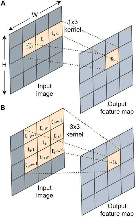
FIGURE 5. Effect of kernel size and the image width on the output feature map for (A) 1D and (B) 2D kernels.

The network architectures are discussed below with the key components provided in Table 3. Each network had three convolution layers. Kernel sizes of 3x3 were used, excluding TS-1D, which used 1x3 kernels as discussed. Zero-padding was used so that the convolution layers did not alter the spatial dimensions of the input. Each convolution layer included rectified linear unit (ReLU) as the activation function, which introduced nonlinearity to system. A pooling layer succeeded each convolution layer, which down-sampled values in the feature maps to reduce the number of parameters and dimensionality of the feature maps. A pooling size and stride of 1x2 was used for the time-series networks, which down-sampled the adjacent points in the signals without distorting the order. A pooling size and stride of 2x2 was used for the time-frequency networks. Dropout was introduced prior to the fully connected layer as a regularization method to prevent overfitting (Srivastava et al., 2014). A dropout rate of 20% was used. Finally, a fully connected layer was used to convert the feature map into a feature vector the size of the number of output variables. A sample network architecture is depicted in Figure 6 for the TS-2D network.

TABLE 3

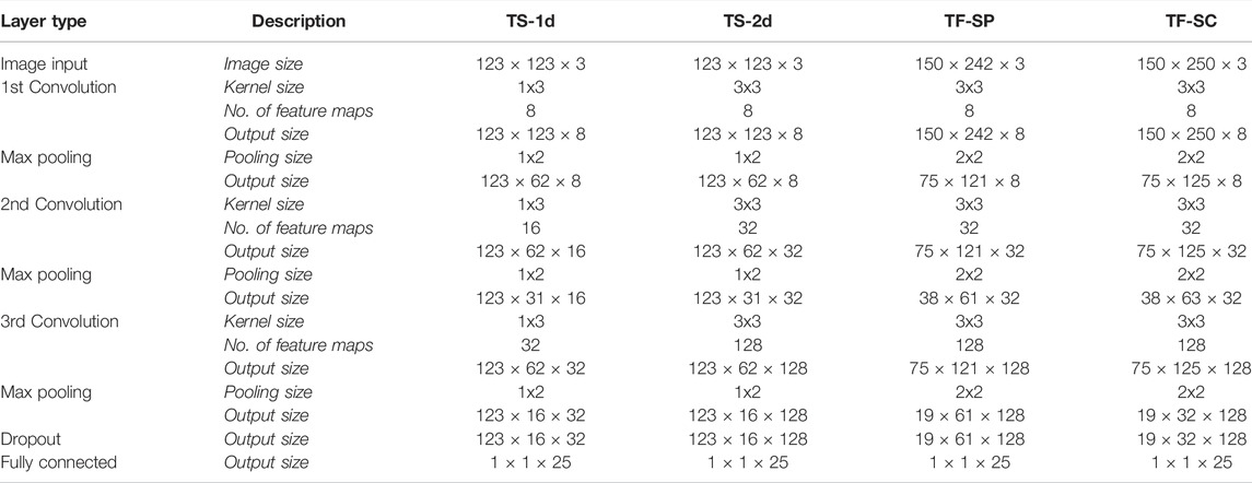
TABLE 3. Architecture details for the four trained networks.

FIGURE 6

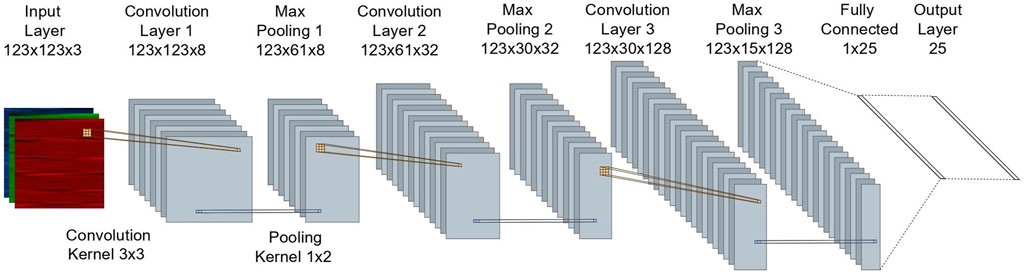
FIGURE 6. Sample architecture for the TS-2D network using the time-series input and 2D kernel.

3.4 Training and Validation

The synthetic dataset was divided into training, validation, and evaluation subsets using an 80/15/5 split. Adaptive moment estimation (Adam) optimization algorithm (Kingma and Ba, 2014) was used with an initial learning rate of 0.001. The learning rate decreased by a factor of 0.1 every 10 epochs. During training, accuracy and loss were calculated using the validation dataset to monitor the progress. Mean-squared-error (MSE) was defined as the loss function. Early stopping was used to automatically terminate training when the current validation loss had exceeded the lowest validation loss 10 times.

3.5 Evaluation Metrics

The four trained networks were compared using the evaluation dataset, which included 5% of the overall synthetic data and was unseen during training. As the individual model parameters do not contribute equally to the global response and different combinations can produce similar force-displacement responses, a set of engineering metrics was defined to provide a more meaningful performance criterion. The defined metrics include the peak lateral force (F_p), residual displacement (δ_r), and cumulative dissipated energy (E). These were selected as they are commonly used to evaluate the seismic design or performance of a bridge column. Additionally, the engineering performance metrics can be used to evaluate the predicted parameters for the experimental data. The engineering metrics are defined in Figure 7 for a representative force-displacement hysteresis curve. For future applications, relevant performance metrics should be selected for evaluation.

FIGURE 7

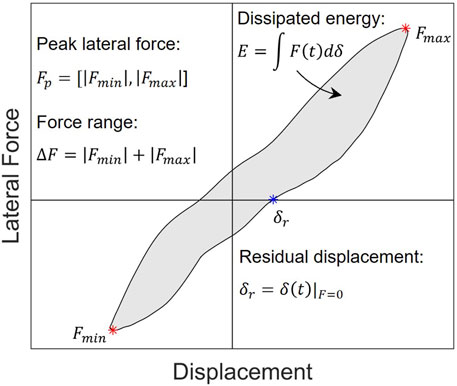
FIGURE 7. Definition of engineering metrics for a sample force-displacement hysteresis loop.

The trained networks were prompted with input data from the evaluate set and the predicted parameters were fed back to the analytical model to generate new simulations. The engineering metrics were calculated from the new analytical responses and compared to the actual values for the original dataset. The mean absolute percentage error (MAPE) was used to calculate the error for the engineering metrics as it is a scale-independent accuracy measure, allowing comparison between the metrics with different units. The MAPE is defined as:

$\text{MAPE}\left(\text{\%}\right)=\frac{100}{n}{\displaystyle \sum }_{i=1}^n\left|\frac{y_a-y_p}{y_a}\right|(1)$

where $y_p$ is the predicted value, $y_a$ is the actual value, and $n$ is the number of samples. The residual displacement was calculated after the largest displacement in the positive and negative loading directions for each run. The average error of the two loading directions was reported for the residual displacement and peak lateral force. As the magnitude of the applied excitations increased throughout the shake table test, the average errors across Runs 1 – 4 and Runs 5 – 7 are reported to compare performance after mid- and high-amplitude excitations.

3.6 Testing Trained Networks With Experimental Data

The model parameters for the composite column system were obtained by prompting the trained network with the lateral load, displacement, and axial load measured during the experimental shake table test. To evaluate the objectivity and sensitivity of the predicted model parameters, the experimental input data was varied by adding GWN with a SNR of 30 dB to the measured time-histories. A total of 10 variations of the experimental data were generated for prompting the trained network. The averages of the predicted values were used in an analytical model to predict the lateral force response of the column system. Finally, the engineering metrics were calculated from the analytical responses and compared to the experimental results to evaluate the accuracy. These steps were completed for each trained network.

4 Results and Discussion

4.1 Performance of the Networks on Synthetic Data

The performance of the four trained networks was assessed using the accuracy capturing the individual model parameters and the defined engineering metrics. The accuracy in predicting the individual model parameters revealed five parameters were not captured by all four of the trained networks. These parameters include the FRP hoop stiffness, E_FRP, hoop rupture strain, ε_FRP, and unloading coefficient, λ, defined for the FRP-confined concrete model, as well as the damping coefficient, C_d, defined in the FRP longitudinal model and the rotational stiffness, k_θ, defined in the FRP-to-concrete bond model. The R² values for these parameters were less than 0.10 across the four networks. The uniform low prediction accuracy for these parameters indicates there was insufficient information in the training data, likely due to the small effect the parameters had on the global response. If calibration of parameters controlling localized behavior is required, additional measurements capturing these effects can be included when training, such as strain gauge measurements. These parameters were not removed from the training data as the small effect on the generated responses served as an additional source of noise, mitigating overfitting. The accuracy capturing the individual model parameters is discussed further in relation to the engineering metrics. The cumulative MSE for the 25 model parameters were 1.11, 1.02, 1.55, and 1.16 for TS-1D, TS-1D, TF-SP, and TF-SC, respectively. The engineering metrics were calculated from the simulated responses given the network predicted parameters, as previously discussed. The MAPE values for the trained networks are compared in Figure 8 for Runs 1—4 and Runs 5—7. The TS-2D network had the lowest average error for the engineering metrics as well as the individual model parameters, followed by TS-1D, TF-SC, and TF-SP, respectively.

FIGURE 8

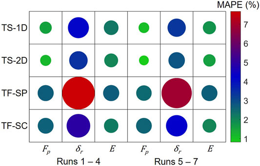
FIGURE 8. Comparison of each trained network in capturing the engineering metrics when prompted with the evaluation dataset. The size and color of the circles are proportional to the error values.

The time-series networks performed notably better on the peak lateral force and residual displacement than the time-frequency networks. Residual displacement is the displacement corresponding to zero force, which requires maintaining information on the relationship between the force and displacement signals, in addition to adequate time resolution that is also required to capture the peak lateral force. This can be accomplished by preserving the order or phase information of the signals. The time-series inputs maintain temporal information as the order and increment of the signals are preserved. While the time-frequency inputs maintain some temporal information, the resolution is limited due to the time-frequency resolution trade-off. As previously discussed, scalograms mitigate this by applying a variable-sized wavelet, allowing TF-SC to outperform TF-SP for residual displacement. The overlapping window length for spectrograms lessens information loss at peaks but does not improve temporal resolution. As such, the accuracy of the time-frequency networks was comparable for the peak lateral force.

The energy dissipation mechanisms in the analytical model were the material hysteretic relationships and Rayleigh damping, which is a form of viscous damping commonly used to approximate the non-hysteretic sources of energy dissipation in structures (Priestley and Grant, 2005; Petrini et al., 2008). Energy dissipation can be measured by the lag between when the displacement reaches its maximum and when the force does, which can be identified in the inputs through temporal shifts between the force and displacement signals. As the Rayleigh damping is also frequency dependent, the time-frequency representations contain additional information that can be used for identification. In the analytical model, the level of Rayleigh damping was primarily controlled by the critical damping ratio, ξ. The hysteretic sources of energy dissipation were controlled by the inelastic material properties, such as the post-cracking shear stiffness, G_cr, and unloading coefficient, β_s, for the shear deformation model. The accuracy in capturing these three model parameters as well as the cumulative energy dissipation, E, is provided in Figure 9, which includes the actual versus predicted values and the corresponding R² value.

FIGURE 9

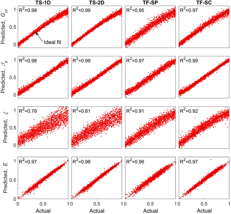
FIGURE 9. Actual versus predicted post-cracking shear stiffness, G_cr, shear deformation unloading coefficient, β_s, damping ratio, ξ_, and cumulative energy dissipation, E, for each representation method.

As shown in Figure 9, the four networks had comparable accuracy for the parameters impacting the hysteretic sources of energy dissipation (G_cr and β_s), which are frequency independent and can be clearly characterized by the force-displacement relationship. However, the time-frequency networks performed considerably better than the time-series networks for the critical damping ratio, as expected due to the frequency-dependent behavior. Despite this, the time-series networks captured the cumulative energy dissipation with comparable accuracy to the time-frequency networks due to the large contribution of material nonlinearity. As such, the time-series networks had higher accuracy for the energy dissipation after the high-amplitude excitation than after the mid-amplitude excitation when there was less material plasticity. This allowed them to outperform the time-frequency networks after the high-level excitation, as shown in Figure 8. The sources of energy dissipation should be considered when selecting the input method.

4.2 Performance in Capturing the Experimentally Measured Response

The model parameters for the composite column system were obtained by prompting the trained network with the experimental data with added random noise as previously discussed. The predicted parameters for the four trained networks were within the range of estimated values from material testing, constitutive equations, or manufacturer specifications. This indicates that the networks did not compensate with unrealistically large or small values when prompted with experimental data. Table 4 includes the predicted values for 11 parameters. These parameters strongly influence the global response and demonstrate key sources of discrepancy between the trained networks. This discrepancy is discussed below in relation to the global response and engineering metrics. The accuracy of the calibrated models in capturing the engineering metrics was also compared to an analytical model previously developed by (Zaghi et al., 2012), referred to herein as the “Reference Model”. The model was developed in OpenSees using conventional calibration approaches, with the full details found in (Zaghi, 2009). The lateral displacement was applied directly to the Reference Model instead of the ground acceleration to facilitate comparison to the current study.

TABLE 4

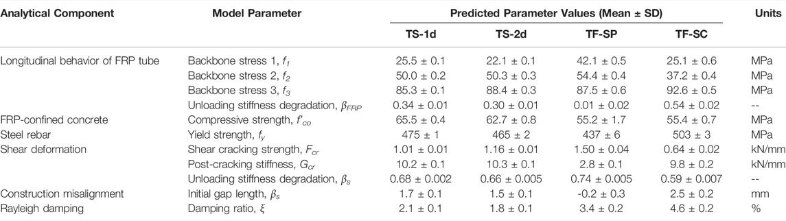
TABLE 4. Predicted values of key model parameters for experimental data with added noise.

The average predicted parameters were fed to the OpenSees analytical model to simulate the response of the composite column. The resulting force-displacement response and corresponding energy dissipation are shown in Figure 10A and Figure 10B, respectively. The energy dissipation was calculated by integrating the measured force-displacement hysteresis curves. The time between cycles was removed for presentation purposes. The R² values were calculated using the predicted force and energy and the measured lateral force and dissipated energy to demonstrate the accuracy across the time histories. The R² values for the lateral force were 0.947, 0.976, 0.852, 0.926, and 0.936 for TS-1D, TS-1D, TF-SP, TF-SC, and the Reference Model, respectively. The R² values for the dissipated energy were 0.993, 0.997, 0.996, 0.924, and 0.831 for TS-1D, TS-1D, TF-SP, TF-SC, and the Reference Model, respectively. Additionally, the engineering metrics were calculated from the analytical responses and compared to the experimental values. The percent error for each metric is compared in Figure 11, including the accuracy of the Reference Model developed by (Zaghi et al., 2012). The color scale axis was set to 50 to facilitate comparison of the smaller errors. Errors over this are reported on the figure.

FIGURE 10

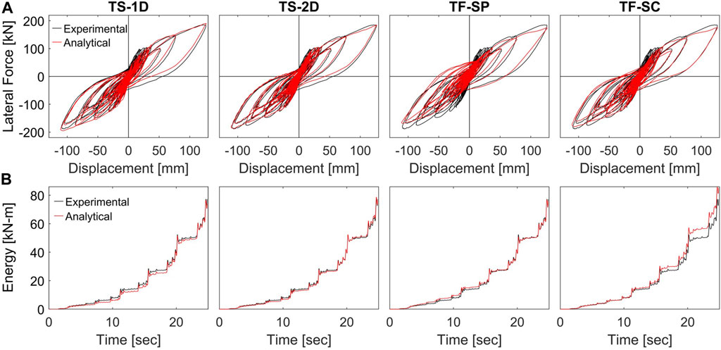
FIGURE 10. Analytical model response given network predicted parameters including (A) global lateral force-displacement and (B) energy dissipation.

FIGURE 11

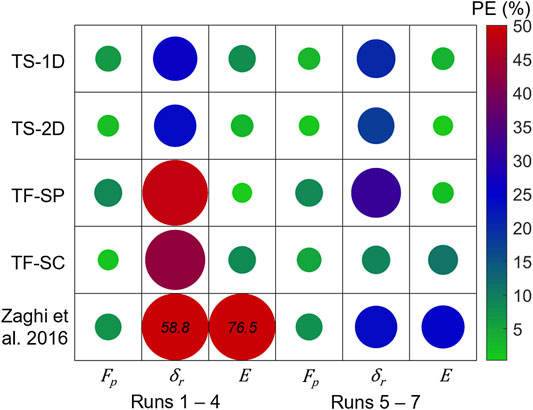
FIGURE 11. Performance of the CNN-predicted model parameters in capturing the engineering metrics when prompted with the experimental data. The size and color of the circles are proportional to the error values.

The accuracy capturing the engineering metrics was generally lower for the experimental data than for the synthetic dataset, which was anticipated as no experimental data was included in training and the analytical model is limited by the approximations in the experimental setup and constitutive relationships. Overall, the trends in performance across the engineering metrics and between the four networks were largely comparable to what was observed for the synthetic dataset. The predicted responses were reasonable for TS-1D, TS-2D, and TF-SC, demonstrating the ability of the networks to generalize to experimental data after training on a synthetic dataset. Additionally, the strong performance of the time-series networks and TF-SC indicate that the framework is applicable to both time-domain and time-frequency domain inputs. The poor performance of TF-SP is likely due to differences between the high frequency artifacts present in the experimental data and synthetic data. This may be mitigated by additional filtering of the predicted responses; however, this may remove information useful during training and is not a necessary step for the other inputs methods. While the strong performance of TF-SC proved the framework is applicable to time-frequency inputs, scalograms require substantially more computation time than the time-series inputs and did not provide substantial improvement in accuracy to justify the use for this application. However, if the objective is calibration of frequency-dependent parameters, using scalograms may be warranted.

The TS-2D network had the lowest errors across the engineering metrics, as shown in Figure 11. Additionally, the difference in performance from the synthetic dataset was smaller for TS-2D than TS-1D. This suggests the 2D kernel provided additional benefit for generalizing to experimental data that was not observed or necessary for the synthetic dataset. The 2D kernel provides information at multiple cycles, such as the loading and unloading slope, which allows TS-2D to balance the contribution of parameters to multiple points of the signal and likely provide more robust feature extraction.

Despite the stronger performance of TS-2D, the time-series networks had comparable predicted parameters with low standard deviations, as shown in Table 4. The time-frequency networks, in contrast, had less consistency between predicted values. A key difference in the predicted parameters is the source of energy dissipation. The time-series networks relied on a similar balance between the hysteretic and non-hysteretic sources of energy dissipation. This is demonstrated by the predicted values for ξ, which controls Rayleigh damping, in comparison to G_cr, β_s, and β_FRP, which control material nonlinearity, shown in Table 4. As the energy dissipation is not provided during training, the time-series networks rely on the relationship between force and displacement to accurately capture the energy dissipation. The time-frequency inputs use frequency-dependent behavior of Rayleigh damping, which allowed for higher accuracy on the synthetic dataset. However, Rayleigh damping is a mathematically convenient method of approximating non-hysteretic sources of energy dissipation and is not directly related to one physical process. To ensure the contribution of hysteretic sources of nonlinearity is accurate, local measurements, such as strain gauges, can be used. Future application of the trained network could be feasible through the use of transfer-learning, which repurposes the trained network to perform a second related task. This could be done to calibrate parameters for a different experimental setup or column geometry. As this requires less training data, this may also be done with experimental data, if available.

The errors for the Reference Model are larger in the early cycles. This was attributed to an underestimation of hysteretic damping at low amplitudes in the analytical model, as noted in (Zaghi et al., 2012). This hysteretic damping is largely due to concrete cracking under small deformations, which was accounted for in the current study through the nonlinear shear model. As a result, the energy dissipation as well as the residual displacements in the low-amplitude cycles were predicted with higher accuracy. Additionally, a high damping ratio of 15% was used in the Reference Model to account for the high damping of the FRP tube and other sources of damping; however, the energy dissipation was still under-predicted. The current model incorporated individual components to represent this (i.e., viscoelastic behavior of the FRP shell and FRP-concrete composite action) and was able to calibrate the additional parameters with the framework. As a result, the energy dissipation was captured across the entire time history with higher accuracy than the Reference Model. Overall, the performance of the Reference Model validates the strong performance of the network predicted parameters.

5 Conclusion

This work proposed a novel supervised learning framework to calibrate the model parameters of complex structural systems with limited experimental data. The framework was evaluated by calibrating the parameters of an analytical model representing the shake table response of a composite column. A CNN was trained using a synthetic dataset to learn the relationships between the analytical model parameters and the displacement, axial load, and analytical lateral load time histories. The applicability of the framework to presenting the signals in both the time-domain and time-frequency domain was investigated. The time-domain input was used to train two CNNs to compare 1D and 2D convolutional kernels. The time-frequency inputs were used to train two CNNs to compare scalograms and spectrograms. Each trained network was prompted with the experimental data from the shake table test to obtain analytical model parameters for the composite column system.

The results of the study demonstrated a CNN can perform parameter calibration for nonlinear dynamic models of structures. When prompted with the experimental data, the trained CNN predicted reasonable model parameters and captured the measured seismic response of the composite column. The accuracy capturing the measured lateral force-displacement response and dissipated energy was higher than the previously developed analytical model for the composite column system. The results demonstrate that a synthetic dataset can be sufficient for training a CNN and the train network can be subsequently used with experimental data without requiring additional training. This indicates additional potential for transfer learning applications using the framework, where it can be retrained with small datasets to performance a related task, such as calibration of a different structural system. Additionally, the results demonstrated image representations of engineering signals are suitable for training CNNs for model calibration of nonlinear structural systems. Presenting the input signals in both the time-domain and time-frequency domain both proved to be a feasible and effective approach for parameter calibration. The networks trained with time-series inputs had lower errors for both the synthetic dataset and the experimental data than for the time-frequency inputs. The time-series inputs also required fewer preprocessing steps and less computation time. Additionally, the time-series inputs benefitted from 2D convolution kernels in place of 1D kernels, which are typically used for signal-processing applications of CNNs. In conclusion, CNN-based parameter calibration presents an effective way of calibrating many parameters of complex structural models with limited experimental data.

Data Availability Statement

The raw data supporting the conclusion of this article will be made available by the authors, without undue reservation.

Author Contributions

AL designed the study, implemented the program, and wrote the initial draft of the manuscript. AE contributed to conception of the study and interpretation of data. TZ contributed to implementation of the program. All authors contributed to manuscript revision, read, and approved the submitted version.

Funding

This project was supported by the National Science Foundation Partnership for Innovation Award #1500293. The student support for this project was funded by the National Science Foundation Graduate Research Fellowship under Grant No. 1747453.

Conflict of Interest

The authors declare that the research was conducted in the absence of any commercial or financial relationships that could be construed as a potential conflict of interest.

Publisher’s Note

All claims expressed in this article are solely those of the authors and do not necessarily represent those of their affiliated organizations, or those of the publisher, the editors, and the reviewers. Any product that may be evaluated in this article, or claim that may be made by its manufacturer, is not guaranteed or endorsed by the publisher.

Acknowledgments

The authors gratefully acknowledged the guidance of Dr. Hadi Meidani of the University of Illinois at Urbana-Champaign. The support of Dr. Alexandra Hain of the University of Connecticut and Michael Vaccaro Jr is also appreciated.

References

Avci, O., Abdeljaber, O., Kiranyaz, S., and Inman, D. (2017). “Structural Damage Detection in Real Time: Implementation of 1D Convolutional Neural Networks for SHM Applications,” in Structural Health Monitoring & Damage Detection (Berlin, Germany: Springer), Vol. 7. doi:10.1007/978-3-319-54109-9_6

CrossRef Full Text | Google Scholar

Balli, T., and Palaniappan, R. (2010). Classification of Biological Signals Using Linear and Nonlinear Features. Physiol. Meas. 31, 903–920. doi:10.1088/0967-3334/31/7/003

PubMed Abstract | CrossRef Full Text | Google Scholar

Bouchikhi, E. H., Choqueuse, V., Benbouzid, M., Charpentier, J.-F., and Barakat, G. (2011). “A Comparative Study of Time-Frequency Representations for Fault Detection in Wind Turbine,” in IECON 2011-37th Annual Conference of the IEEE Industrial Electronics Society, Melbourne, Australia, November 7–10, 2011 (IEEE), 3584–3589. doi:10.1109/iecon.2011.6119891

CrossRef Full Text | Google Scholar

Burgueño, R., and Bhide, K. M. (2006). Shear Response of concrete-filled FRP Composite Cylindrical Shells. J. Struct. Eng. 132, 949–960. doi:10.1061/(ASCE)0733-9445(2006)132:6(949)

CrossRef Full Text | Google Scholar

Carreño, R., Lotfizadeh, K., Conte, J., and Restrepo, J. (2020). Material Model Parameters for the Giuffrè-Menegotto-Pinto Uniaxial Steel Stress-Strain Model. J. Struct. Eng. 146, 04019205. doi:10.1061/(ASCE)ST.1943-541X.0002505

CrossRef Full Text | Google Scholar

Cerna, M., and Harvey, A. F. (2000). The Fundamentals of FFT-Based Signal Analysis and Measurement. Application Note 041. Austin, TX: National Instruments Corporation.

Google Scholar

Chen, J., Wan, L., Ismail, Y., Ye, J., and Yang, D. (2021). A Micromechanics and Machine Learning Coupled Approach for Failure Prediction of Unidirectional CFRP Composites under Triaxial Loading: A Preliminary Study. Compos. Structures 267, 113876. doi:10.1016/j.compstruct.2021.113876

CrossRef Full Text | Google Scholar

Chen, Y.-Y., and Wang, Z.-B. (2019). Feature Selection Based Convolutional Neural Network Pruning and its Application in Calibration Modeling for NIR Spectroscopy. Chemometrics Intell. Lab. Syst. 191, 103–108. doi:10.1016/j.chemolab.2019.06.004

CrossRef Full Text | Google Scholar

Cohen, L. (1995). Time-frequency Analysis. Englewood Cliffs, NJ: Prentice-Hall.

Google Scholar

Filippou, F. C., Bertero, V. V., and Popov, E. P. (1983). Effects of Bond Deterioration on Hysteretic Behavior of Reinforced concrete Joints. Berkeley, California: Earthquake Engineering Research Center.

Google Scholar

Gandomi, A. H., Babanajad, S. K., Alavi, A. H., and Farnam, Y. (2012). Novel Approach to Strength Modeling of concrete under Triaxial Compression. J. Mater. Civ. Eng. 24, 1132–1143. doi:10.1061/(asce)mt.1943-5533.0000494

CrossRef Full Text | Google Scholar

Hauksson, E., Jones, L. M., and Hutton, K. (1995). The 1994 Northridge Earthquake Sequence in California: Seismological and Tectonic Aspects. J. Geophys. Res. 100, 12335–12355. doi:10.1029/95jb00865

CrossRef Full Text | Google Scholar

Hoang, D.-T., and Kang, H.-J. (2017). “Convolutional Neural Network Based Bearing Fault Diagnosis,” in International conference on intelligent computing, Liverpool, UK, August 7–10, 2017 (Springer), 105–111. doi:10.1007/978-3-319-63312-1_9

CrossRef Full Text | Google Scholar

Huang, H., and Burton, H. V. (2019). Classification of In-Plane Failure Modes for Reinforced concrete Frames with Infills Using Machine Learning. J. Building Eng. 25, 100767. doi:10.1016/j.jobe.2019.100767

CrossRef Full Text | Google Scholar

Ilkhani, M. H., Naderpour, H., and Kheyroddin, A. (2019). A Proposed Novel Approach for Torsional Strength Prediction of RC Beams. J. Building Eng. 25, 100810. doi:10.1016/j.jobe.2019.100810

CrossRef Full Text | Google Scholar

Kang, M.-C., Yoo, D.-Y., and Gupta, R. (2021). Machine Learning-Based Prediction for Compressive and Flexural Strengths of Steel Fiber-Reinforced concrete. Construction Building Mater. 266, 121117. doi:10.1016/j.conbuildmat.2020.121117

CrossRef Full Text | Google Scholar

Khan, A., Ko, D.-K., Lim, S. C., and Kim, H. S. (2019). Structural Vibration-Based Classification and Prediction of Delamination in Smart Composite Laminates Using Deep Learning Neural Network. Composites B: Eng. 161, 586–594. doi:10.1016/j.compositesb.2018.12.118

CrossRef Full Text | Google Scholar

Khare, S. K., and Bajaj, V. (2020). Time-frequency Representation and Convolutional Neural Network-Based Emotion Recognition. IEEE Trans. Neural networks Learn. Syst. 32 (7), 2901–2909.

PubMed Abstract | CrossRef Full Text | Google Scholar

Kim, B., Jeong, H., Kim, H., and Han, B. (2017). Exploring Wavelet Applications in Civil Engineering. KSCE J. Civ Eng. 21, 1076–1086. doi:10.1007/s12205-016-0933-3

CrossRef Full Text | Google Scholar

Kingma, D. P., and Ba, J. (2014). “Adam: A Method for Stochastic Optimization” in 3rd International Conference for Learning Representations (ICLR), San Diego, US, May 7–9, 2015. arXiv preprint arXiv:1412.6980.

Google Scholar

Kiranyaz, S., Ince, T., Hamila, R., and Gabbouj, M. (2015). “Convolutional Neural Networks for Patient-specific ECG Classification,” in 37th Annual International Conference of the IEEE Engineering in Medicine and Biology Society (EMBC), 2015, Milano, Italy, August 25–29, 2015 (IEEE), 2608–2611. doi:10.1109/EMBC.2015.7318926

PubMed Abstract | CrossRef Full Text | Google Scholar

Kiranyaz, S., Avci, O., Abdeljaber, O., Ince, T., Gabbouj, M., and Inman, D. J. (2021). 1D Convolutional Neural Networks and Applications: A Survey. Mech. Syst. Signal Process. 151, 107398. doi:10.1016/j.ymssp.2020.107398

CrossRef Full Text | Google Scholar

Kolar, D., Lisjak, D., Pająk, M., and Pavković, D. (2020). Fault Diagnosis of Rotary Machines Using Deep Convolutional Neural Network with Wide Three axis Vibration Signal Input. Sensors 20, 4017. doi:10.3390/s20144017

PubMed Abstract | CrossRef Full Text | Google Scholar

Kong, X., Cai, C. S., Deng, L., and Zhang, W. (2017). Using Dynamic Responses of Moving Vehicles to Extract Bridge Modal Properties of a Field Bridge. J. Bridge Eng. 22, 04017018. doi:10.1061/(asce)be.1943-5592.0001038

CrossRef Full Text | Google Scholar

Kulkarni, S. M., and Shah, S. P. (1998). Response of Reinforced concrete Beams at High Strain Rates. Struct. J. 95, 705–715. doi:10.14359/584

CrossRef Full Text | Google Scholar

Lilly, J. M. (2017). Element Analysis: a Wavelet-Based Method for Analysing Time-Localized Events in Noisy Time Series. Proc. R. Soc. A. 473, 20160776. doi:10.1098/rspa.2016.0776

PubMed Abstract | CrossRef Full Text | Google Scholar

Lilly, J. M., and Olhede, S. C. (2012). Generalized Morse Wavelets as a Superfamily of Analytic Wavelets. IEEE Trans. Signal. Process. 60, 6036–6041. doi:10.1109/tsp.2012.2210890

CrossRef Full Text | Google Scholar

Lilly, J. M., and Olhede, S. C. (2008). Higher-order Properties of Analytic Wavelets. IEEE Trans. Signal Process. 57, 146–160. doi:10.1109/TSP.2008.2007607

CrossRef Full Text | Google Scholar

Liu, X., Gasco, F., Goodsell, J., and Yu, W. (2019). Initial Failure Strength Prediction of Woven Composites Using a New Yarn Failure Criterion Constructed by Deep Learning. Compos. Structures 230, 111505. doi:10.1016/j.compstruct.2019.111505

CrossRef Full Text | Google Scholar

Matoušek, J. (1998). On Thel2-Discrepancy for Anchored Boxes. J. Complexity 14, 527–556. doi:10.1006/jcom.1998.0489

CrossRef Full Text | Google Scholar

Mazzoni, S., Mckenna, F., Scott, M. H., and Fenves, G. L. (2009). OpenSees Command Language Manual. Berkeley: Pacific Earthquake Engineering Research Center, University of California.

Google Scholar

Murad, Y., Hunifat, R., and Wassel, A.-B. 2020. “Interior Reinforced Concrete Beam-to-Column Joints Subjected to Cyclic Loading: Shear Strength Prediction Using Gene Expression Programming.” Case Stud. Constr. Mater. 13, e00432. doi:10.1016/j.cscm.2020.e00432

CrossRef Full Text | Google Scholar

Naderpour, H., Sharei, M., Fakharian, P., and Heravi, M. A. (2022). Shear Strength Prediction of Reinforced Concrete Shear Wall Using ANN, GMDH-NN and GEP. Soft Comput. Civil Eng. 6, 66–87. doi:10.22115/SCCE.2022.283486.1308

CrossRef Full Text | Google Scholar

Nagarajaiah, S., and Basu, B. (2009). Output Only Modal Identification and Structural Damage Detection Using Time Frequency & Wavelet Techniques. Earthq. Eng. Eng. Vib. 8, 583–605. doi:10.1007/s11803-009-9120-6

CrossRef Full Text | Google Scholar

Petrini, L., Maggi, C., Priestley, M. J. N., and Calvi, G. M. (2008). Experimental Verification of Viscous Damping Modeling for Inelastic Time History Analyzes. J. Earthquake Eng. 12, 125–145. doi:10.1080/13632460801925822

CrossRef Full Text | Google Scholar

Pham, M. T., Kim, J.-M., and Kim, C. H. (2020). Accurate Bearing Fault Diagnosis under Variable Shaft Speed Using Convolutional Neural Networks and Vibration Spectrogram. Appl. Sci. 10, 6385. doi:10.3390/app10186385

CrossRef Full Text | Google Scholar

Priestley, M. J. N., and Grant, D. N. (2005). Viscous Damping in Seismic Design and Analysis. J. earthquake Eng. 9, 229–255. doi:10.1142/s1363246905002365

CrossRef Full Text | Google Scholar

Rafiei, M. H., Khushefati, W. H., Demirboga, R., and Adeli, H. (2016). Neural Network, Machine Learning, and Evolutionary Approaches for Concrete Material Characterization. ACI Mater. J. 113, 781–789. doi:10.14359/51689360

CrossRef Full Text | Google Scholar

Rochac, J. F. R., Zhang, N., Xiong, J., Zhong, J., and Olandunni, T. (2019). “Data Augmentation for Mixed Spectral Signatures Coupled With Convolutional Neural Networks” in 9th International Conference on Information Science and Technology (ICIST) (Hulunbuir, China: IEEE), 402–407. doi:10.1109/ICIST.2019.8836868

CrossRef Full Text | Google Scholar

Sadoughi, M., and Hu, C. (2019). Physics-based Convolutional Neural Network for Fault Diagnosis of Rolling Element Bearings. IEEE Sensors J. 19, 4181–4192. doi:10.1109/jsen.2019.2898634

CrossRef Full Text | Google Scholar

Shao, Y. (2003). Behavior of FRP-Concrete Beam-Columns Under Cyclic Loading. Raleigh, NC: North Carolina State University.

Google Scholar

Silik, A., Noori, M., A. Altabey, W., Ghiasi, R., and Wu, Z. (2021). Comparative Analysis of Wavelet Transform for Time-Frequency Analysis and Transient Localization in Structural Health Monitoring. Struct. Durability Health Monit. 15, 1–22. doi:10.32604/sdhm.2021.012751

CrossRef Full Text | Google Scholar

Skublska-Rafajłowicz, E., and Rafajłowicz, E. (2012). Sampling Multidimensional Signals by a New Class of Quasi-Random Sequences. Multidimensional Syst. Signal Process. 23, 237–253. doi:10.1007/s11045-010-0120-5

CrossRef Full Text | Google Scholar

Sobol', I. Y. M. (1967). On the Distribution of Points in a Cube and the Approximate Evaluation of Integrals. Zhurnal Vychislitel'noi Matematiki i Matematicheskoi Fiziki 7, 784–802. doi:10.1016/0041-5553(67)90144-9

CrossRef Full Text | Google Scholar

Spanos, P. D., Giaralis, A., and Politis, N. P. (2007). Time-frequency Representation of Earthquake Accelerograms and Inelastic Structural Response Records Using the Adaptive Chirplet Decomposition and Empirical Mode Decomposition. Soil Dyn. Earthquake Eng. 27, 675–689. doi:10.1016/j.soildyn.2006.11.007

CrossRef Full Text | Google Scholar

Srivastava, N., Hinton, G., Krizhevsky, A., Sutskever, I., and Salakhutdinov, R. (2014). Dropout: a Simple Way to Prevent Neural Networks from Overfitting. J. machine Learn. Res. 15, 1929–1958.

Google Scholar

Systems, N. F. G. (2012). Red Thread II Piping Systems. San Antonio, TX: National Oilwell Varco.

Google Scholar

Tang, C.-W. (2010). Radial Basis Function Neural Network Models for Peak Stress and Strain in plain concrete under Triaxial Stress. J. Mater. Civ. Eng. 22, 923–934. doi:10.1061/(asce)mt.1943-5533.0000077

CrossRef Full Text | Google Scholar

Teng, J. G., Jiang, T., Lam, L., and Luo, Y. Z. (2009). Refinement of a Design-Oriented Stress-Strain Model for FRP-Confined Concrete. J. Compos. Constr. 13, 269–278. doi:10.1061/(asce)cc.1943-5614.0000012

CrossRef Full Text | Google Scholar

Wang, Y., Zhou, J., Zheng, L., and Gogu, C. (2020). An End-To-End Fault Diagnostics Method Based on Convolutional Neural Network for Rotating Machinery with Multiple Case Studies. J. Intell. Manufacturing 33, 1–22. doi:10.1007/s10845-020-01671-1

CrossRef Full Text | Google Scholar

Wang, Z., Zhao, W., Du, W., Li, N., and Wang, J. (2021). Data-driven Fault Diagnosis Method Based on the Conversion of Erosion Operation Signals into Images and Convolutional Neural Network. Process Saf. Environ. Prot. 149, 591–601. doi:10.1016/j.psep.2021.03.016

CrossRef Full Text | Google Scholar

Willard, J., Jia, X., Xu, S., Steinbach, M., and Kumar, V. (2020). Integrating Physics-Based Modeling with Machine Learning: A Survey. ACM Comput. Surv. 1 (1), 1–34. arXiv preprint arXiv:2003.04919. doi:10.48550/arXiv.2003.04919

CrossRef Full Text | Google Scholar

Wilson, E. L. (2004). Static and Dynamic Analysis of Structures, in A Physical Approach with Emphasis on Earthquake Enginering. 4th Edn. Berkeley, CA: Computers and Structures Inc..

Google Scholar

Xu, C., Guan, J., Bao, M., Lu, J., and Ye, W. (2018). Pattern Recognition Based on Time-Frequency Analysis and Convolutional Neural Networks for Vibrational Events in φ-OTDR. Opt. Eng. 57, 016103. doi:10.1117/1.oe.57.1.016103

CrossRef Full Text | Google Scholar

Yan, S., Zou, X., Ilkhani, M., and Jones, A. (2020). An Efficient Multiscale Surrogate Modelling Framework for Composite Materials Considering Progressive Damage Based on Artificial Neural Networks. Composites Part B: Eng. 194, 108014. doi:10.1016/j.compositesb.2020.108014

CrossRef Full Text | Google Scholar

Yu, Y., Wang, C., Gu, X., and Li, J. (2019). A Novel Deep Learning-Based Method for Damage Identification of Smart Building Structures. Struct. Health Monit. 18, 143–163. doi:10.1177/1475921718804132

CrossRef Full Text | Google Scholar

Zadeh, M., and Saiidi, M. (2007). Effect of Constant and Variable Strain Rates on Stress-Strain Properties and Yield Propagation in Steel Reinforcing Bars. Report No. CCEER-07-2 (Reno: Center for Civil Engineering Earthquake Research, University of Nevada).

Google Scholar

Zaghi, A. E., Saiidi, M. S., and Mirmiran, A. (2012). Shake Table Response and Analysis of a concrete-filled FRP Tube Bridge Column. Compos. Structures 94, 1564–1574. doi:10.1016/j.compstruct.2011.12.018

CrossRef Full Text | Google Scholar

Zaghi, A. E. (2009). Seismic Design of Pipe-Pin Connections in concrete Bridges. Reno: University of Nevada.

Google Scholar

Zare, S., and Ayati, M. (2021). Simultaneous Fault Diagnosis of Wind Turbine Using Multichannel Convolutional Neural Networks. ISA Trans. 108, 230–239. doi:10.1016/j.isatra.2020.08.021

PubMed Abstract | CrossRef Full Text | Google Scholar

Zhang, W., Peng, G., and Li, C. (2017). “Bearings Fault Diagnosis Based on Convolutional Neural Networks with 2-D Representation of Vibration Signals as Input,” in 2016 the 3rd International Conference on Mechatronics and Mechanical Engineering, Shanghai, China, October 21–23, 2016 (Shanghai, China: EDP Sciences), 13001. doi:10.1051/matecconf/20179513001

CrossRef Full Text | Google Scholar

Zhang, Y., Xing, K., Bai, R., Sun, D., and Meng, Z. (2020). An Enhanced Convolutional Neural Network for Bearing Fault Diagnosis Based on Time-Frequency Image. Measurement 157, 107667. doi:10.1016/j.measurement.2020.107667

CrossRef Full Text | Google Scholar

Zhu, Z., Ahmad, I., and Mirmiran, A. (2006). Fiber Element Modeling for Seismic Performance of Bridge Columns Made of concrete-filled FRP Tubes. Eng. structures 28, 2023–2035. doi:10.1016/j.engstruct.2006.03.031

CrossRef Full Text | Google Scholar

Zuhair Murad, Y. (2021). Predictive Model for Bidirectional Shear Strength of Reinforced concrete Columns Subjected to Biaxial Cyclic Loading. Eng. Structures 244, 112781. doi:10.1016/j.engstruct.2021.112781

CrossRef Full Text | Google Scholar