Dam-Break Waves’ Hydrodynamics on Composite Bathymetry

1 Introduction

Tsunamis are recurring, devastating natural disasters that vulnerable regions can hardly shelter from. They frequently cause numerous casualties and considerable damage to economic assets, as demonstrated by the Indian Ocean tsunami in 2004 (Borrero et al., 2006; Fritz et al., 2006a; Ghobarah et al., 2006; Goff et al., 2006; Jaffe et al., 2006; Rodriguez et al., 2006; Saatcioglu et al., 2006; Tomita et al., 2006), the Chilean tsunami in 2010 (Fritz et al., 2011; Palermo et al., 2013), the Japanese tsunami in 2011 (von Hippel, 2011; Mikami et al., 2012; Chock et al., 2013; Satake et al., 2013; Mori et al., 2014), or the 2018 Indonesian tsunami (Mikami et al., 2019; Paulik et al., 2019; Aránguiz et al., 2020; Stolle et al., 2020; Krautwald et al., 2021). To improve predictions and estimations as to the damage potential of these extreme hydrodynamic events, research is ongoing and carried out by a large group of scientists all over the world. The overarching ambition is to understand the effects and implications of tsunamis more comprehensively; this happens in order to minimize the severe consequences of a tsunami disaster by optimizing evacuation concepts (e.g., Taubenböck et al., 2009) or refining standards (e.g., Naito et al., 2014).

1.1 Literature Review on Dam-Break Waves as an Analogy to Tsunami Waves

Tsunami waves are often caused by tectonic events, usually originating from seabed displacements at larger water depths. In combination with their wave length, they are predominantly shallow-water waves by definition. While propagating in the deep ocean, tectonic tsunamis have small wave heights and usually cause no damage. They can often be detected by early warning systems facilitating pressure sensors on the seafloor (DART system, Bernard and Titov, 2015). More recent attempts have used satellite altimetry to detect tsunamis in deep water (Ablain et al., 2006). Once reaching shallower waters, shoaling increases the wave height while the wave gets shorter and more devastating. Wave breaking occurs mostly prior to landfall and undular bores might develop (Matsuyama et al., 2007; Grue et al., 2008).

Storm waves, which are much shorter than tsunamis, can be simulated almost in their original scale in the largest wave flumes in the world equipped with flap or piston-type wave makers (Oumeraci, 2010). These facilities are also capable of generating solitary or N-waves, which have been often used in simulating tsunami waves. However, even though leading solitary-like waves might reach the shoreline first, Madsen et al. (2008) revealed in a comprehensive study that solitary waves as a model are inappropriate to represent the bulk tsunami on its geophysical scale by affirming that they are “magnitudes” too short. Later on, in 2010, Madsen and Schäffer (2010) conclude that from its generation in the ocean to its impact at the shore, the relevant length- and time-scales of the bulk tsunami are never defined by the solitary wave tie, that is, given by the ratio of the wave height to the water depth. In 2012, Chan and Liu (2012) relax the statement that a solitary wave is “magnitudes” too short (Madsen et al., 2008) by analyzing the time history of an offshore buoy affected by the Tohoku tsunami. They found that in this case, a solitary wave would be approximately six times too short but not magnitudes. However, generating sufficiently long waves is not (or only on a small scale) possible in common wave flumes due to the limited stroke of these facilities. Hence, pump-driven wave generators are often used to cope with this limitation (Goseberg et al., 2013; Park et al., 2013; Schimmels et al., 2016; Sriram et al., 2016; Tomiczek et al., 2016). In line with Madsen et al. (2008) and Madsen and Schäffer (2010), Chanson (2006) suggested using dam-break waves in analogy to tsunami waves propagating on-shore and proposed an analytical two-dimensional (2D) model to calculate dam-break waves of real fluids, including friction. This author found good agreement between calculations and observations made by video cameras during the 2004 Banda Ache tsunami (Chanson, 2006).

Similar to tsunami inundation, dam-break waves are characterized by a quasi-infinite wavelength, increasing water level over time and simultaneously decreasing depth-averaged flow velocities. Ritter (1897) first derived equations to describe the surface, depth-averaged velocity, and wave tip celerity of an ideal fluid dam-break wave in a horizontal, initially dry flume. However, his equations do not consider friction. Addressing this issue, Dressler (1952) used the Chezy resistance coefficient to propose an improved approximation. Whitham and Lighthill (1955) adapted the Ritter (1897) solution to consider friction in the wavefront tip region, where friction and turbulence cause the wavefront to slow down and thicken. A more recent analytical solution was presented by Chanson (2009) who additionally included a variable Darcy friction factor for the wave tip region and successfully validated the model against large-scale experimental data. The latter solution is applicable to horizontal and sloping channels.

In laboratory testing, dam-break waves are commonly generated by lift or swing gates, either driven by rapidly opening actuators (von Häfen et al., 2018; von Häfen et al., 2019) or using the vertical release method where an elevated reservoir is quickly emptied into a lower basin that is again connected to a propagation flume (Wüthrich et al., 2018).

Some authors investigated dam-break waves propagating on sloped bathymetry. Mostly, past studies focused on the wave propagating down an inclined bottom in analogy to a dam-break wave triggered by a bursting river dam in the mountains rushing down into the valley (positively inclined slope), while few others focused their work on dam-break waves propagating up an inclined bottom, this then in analogy to a tsunami wave inundating a site with rising topography (negatively inclined slope). Studies dealing with positively inclined slopes are not in the scope of this thesis. The interested reader is referred to Dressler and Stoneley (1958), Hunt (1983), Hunt (1984), Nsom et al. (2000), Fernandez-Feria (2006), and Chanson (2009), who proposed the previously mentioned analytical solution to describe the dam-break wave celerity and surface in a positively or negatively inclined channel. Among others, studies dealing with dam-break wave propagation on negatively inclined slopes are those of Yeh et al. (1989) and Yeh (1991) who investigated broken bores running up a slope in laboratory experiments. These authors used water on both sides of a lift gate in initial settings and a constant slope angle of 7.5°. Once the gate was opened, the dam-break wave slumped into the resting water downstream of the gate. Yeh et al. (1989) and Yeh (1991) observed a so-called “momentum exchange” between the dam-break wave and the resting water downstream of the gate and found that the resting water is pushed up the slope first, followed by the bore. Lu et al. (2018) conducted experimental tests similar to those of Yeh et al. (1989) and Yeh (1991) but using a larger distance between the gate and the toe of the slope ($0.4 \text{m}$ vs. $1.8 \text{m}$). They found a linear relationship with a uniform gradient between impoundment depth and maximum run-up height. Also, given the same impoundment depth, the run-up height increases with increasing initial water depth downstream of the gate. Hence, run-up height is the smallest for an initially dry flume. Furthermore, Lu et al. (2018) analyzed the spatiotemporal development of the run-up process in detail. Barranco and Liu (2021) generated dam-break waves in a flume with water on both sides of the dam-break gate and used a variable reservoir length to investigate the features of the waves’ run-up. They found a dependency between the run-up height and the initial impoundment depth and flood duration. By facilitating a numerical model, they proposed equations to predict the inundation depth, run-up height, and duration of the flood in relation to the bore characteristics (Barranco and Liu, 2021).

Following Chanson (2006) and Madsen et al. (2008), dam-break waves are frequently used by a multitude of authors in the context of tsunami engineering: Derschum et al. (2018), Khan et al. (2000), Stolle et al. (2018), Stolle et al. (2019), Stolle et al. (2020b), Stolle et al. (2020a), and von Häfen et al. (2021) used dam-break waves to study debris transport and debris-induced loadings, and Nistor et al. (2017a), Nistor et al. (2017b), Stolle et al. (2016), and Wüthrich et al. (2020) used the vertical release method to investigate debris motion as well. Al-Faesly et al. (2012), Arnason et al. (2009), Aureli et al. (2015), Cross (1967), Farahmandpour et al. (2020), Moon et al. (2019), Ramsden (1996), Shafiei et al. (2016), Soares-Frazão and Zech (2007), Soares-Frazão and Zech (2008), Winter Andrew et al. (2021), and Xu et al. (2020) used dam-break waves to investigate loads on structures like residential houses, breakwaters or idealized cities, and the associated flow regime. Kuswandi and Triatmadja (2019), Maqtan et al. (2018), and Triatmadja et al. (2011) used dam-break waves to investigate scouring around structures during tsunami inundations.

Since tsunami forecasting is challenging and only allows for a short-term warning, evacuation plans need to be applied rapidly after a tsunami hazard is detected (Taubenböck et al., 2013), and no measuring equipment can be installed before the wave reaches the site. Therefore, very limited measurements of flow depths and velocities of real-world tsunami events exist. Fritz et al. (2006b) analyzed survivor videos taken during the 2004 Banda Aceh tsunami. Both survivors observed sites about $3 \text{km}$ inland; one in downtown Banda Aceh, and one in a residential area. Extensive image processing and referencing allowed for extracting surface velocimetry and flow depth from the camera feeds. Fritz et al. (2006b) calculated the Froude numbers for both sites and found that they are close to $F_r = 1.0$. Matsutomi et al. (2010) analyzed field data of several tsunami events and calculated Froude numbers in the range of $F_r =$ 0.42–2.0 (also depending on velocity estimation). Chanson (2006) also used camera footage from the Banda Ache tsunami in 2004 to validate his analytical dam-break wave approach and highlights the importance of real-fluid bottom-friction interaction. He reports a wavefront velocity of about 1.5 to $1.6 \text{m}/\text{s}$ at a site located about 1.5 to $3.0 \text{km}$ inland. Fritz et al. (2012) conducted field surveys in 2011 in Kesennuma Bay (Japan), which was heavily affected by the Tohoku tsunami. They used video recordings taken during the inundation and calibrated them with real-world coordinates measured in field surveys. Focusing on the hydrodynamics in the Kesennuma Bay narrows, they report a wave trough of $-3\text{ m}$ followed by 12 min of flooding with a wave crest height of up to $9\text{ m}$ before the flow direction reverses into an outflow. Observed standing water surface waves within the navigation channel (typical water depth of $10\text{ m}$) support the finding that the Froude number, extracted from the camera recordings, approached approximately unity.

1.2 Identified Knowledge Gaps, Objectives, and Aspects of Novelty

Dam-break waves are widely used to simulate tsunami hydrodynamics, both in numerical and physical tests. This is due to their ability to mimic some relevant features that govern tsunami wave hydrodynamics, such as their very long wavelength. In addition to the applications in the field of tsunami-related research, dam-break waves are frequently used in numerical fluid modeling as it is a common test case to validate the accuracy of numerical formulation. Also, numerous publications exist dealing with the obvious analogy to breaking river dams and the associated flood wave. Due to their wide field of application, a multitude of approximations and analytical solutions exists, predicting the surface elevation and flow features of dam-break waves.

However, the aforementioned literature review on tsunami-related applications revealed a lack of knowledge regarding dam-break waves propagation over a sloping bathymetry adjacent to a horizontal plane (composite bathymetry) in analogy to a tsunami wave reaching a sloping bathymetry, approaching a shore, and subsequently inundating a horizontal site (see Figure 1). To date, it remains unclear how the dam-break-induced flow evolves after it has climbed the slope and then suddenly being exposed to a change in inclination.

FIGURE 1

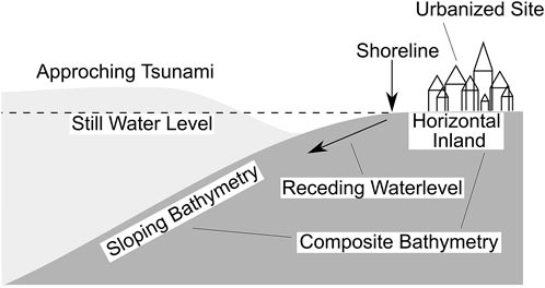
FIGURE 1. Conceptual sketch of a tsunami wave propagating on a sloped bathymetry while approaching the shore. The inland topography is approximately horizontal (composite bathymetry). The still water line is indicated by a dashed line. Note that a tsunami not necessarily consists of a leading trough, as shown here, when approaching the shore (Fritz et al., 2006a).

This study, hence, intends to shed light on the features of a dam-break waves’ overland flow. Previous studies on tsunami effects, where dam-break waves have been used, did simply set a specific distance between the dam-break gate and their test setup; very rarely was that distance discussed. However, the surface elevation $\eta$ is a function of space $x$ and time $t$ with the largest gradients for small $x$ (von Häfen et al., 2019). This study, hence, also aims to raise awareness of the fact that the distance parameter $x$ has to be taken into account when planning dam-break-based laboratory tests in analogy to tsunami waves.

This study presents a unique, novel set of physical large-scale dam-break tests propagating over a composite bathymetry; the data set is subsequently used to calibrate a high-resolution numerical model. That model is then used to analyze the parameters governing the hydrodynamics. The following specific objectives are addressed within this study:

1) To raise awareness of and quantify the dam-break waves’ changing hydrodynamics over space and time using simple analytical considerations.

2) To introduce qualitative categories (referred to as classes) to describe types of flow patterns observed and gained through an extensive numerical parameter study.

3) To correlate the classes with the governing parameters varied within the parameter study.

4) To describe the flow features quantitatively (flow depth, velocity, and Froude number) of the dam-break wave affected by the composite bathymetry over space and time and link them to the qualitative categories (classes) to gain knowledge about the underlying physics.

5) To provide empirical equations to predict the overland flow features.

Although there might be additional interest in the sloping region of the composite slope, this study focuses specifically on the flow characteristics along the horizontal plane, as it represents the region where urban siting would typically be present (see Figure 1). The authors deem this region mostly important since improving knowledge in this area is of great interest for reducing the number of severe losses caused by a tsunami event.

2 Methodology

2.1 Laboratory Experiments

Laboratory experiments are conducted to calibrate and validate the numerical model Reef3D (see Section 2.2). The test facility is situated at the Leichtweiß-Institute for Hydraulic Engineering and Water Resources, Technische Universität Braunschweig, Germany. The flume used for the dam-break experiments is 2 m wide and approximately 100 m long. A swing gate separates the flume into a 20-m long reservoir section, where water is impounded, and an 80-m long propagation section. The gate is driven by an electric linear drive, which allows a fully controllable movement of the gate. The gate opens within 0.7 s ensuring an unaffected, quasi-instantaneous dam-break (comparable to the ideal numerical dam-break used within this study, see Section 2-3), leading to a dam-break bore propagating downstream the flume (von Häfen et al., 2019). The flume is equipped with four wave gauges, capacity type (200 Hz, accuracy ∼1%, tailor-made). One of the gauges is located in the reservoir and three downstream the gate in the propagation section of the flume whose positions are indicated in Figure 2. Wave gauges and linear drive are synchronized using a data acquisition system (ADLINK DAQe-2206, 64 channel, 16 bit, 250 kS/s). Capacitance wave gauges have been used successfully in accurately detecting aerated flows as occurring during advancing broken bores (Derschum et al., 2018; Ghodoosipour et al., 2019; Stolle et al., 2019a; Stolle et al., 2019b). Figure 2 shows the flume including a composite bathymetry and measuring devices. Wave reflection at the end of the flume is not recorded by the data acquisition system since the length of the flume is sufficient to stop the measurements before a reflection arrives.

FIGURE 2

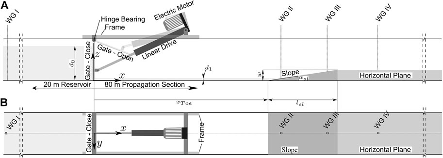
FIGURE 2. Dam-break facility equipped with a fully controllable gate and four wave gauges in side- (A) and top-view (B). The composite bathymetry and the parameters describing its geometry are indicated.

For calibration and validation purposes, four experimental tests are conducted: two with a flat bottom and two with a composite bathymetry installed. Each of these four tests is repeated twice. Table 1 contains the experimental protocol including the impoundment depth $d_0$ and the positions of the wave gauges. In the case of an installed composite slope (test nos. 3 & 4), the distance between the gate and toe of the slopes $x_{toe}$ is given, as well as the parameters describing the slope geometry; the height of the horizontal plane $w$ and slope length $l_{sl}$ (see Figure 2). A numerical model (see Section 2.3) is calibrated using the flat bottom test no. 1 (see Table 1) and validated later on against the remaining tests with (no. 2) and without the composite bathymetry (nos. 3 & 4).

TABLE 1

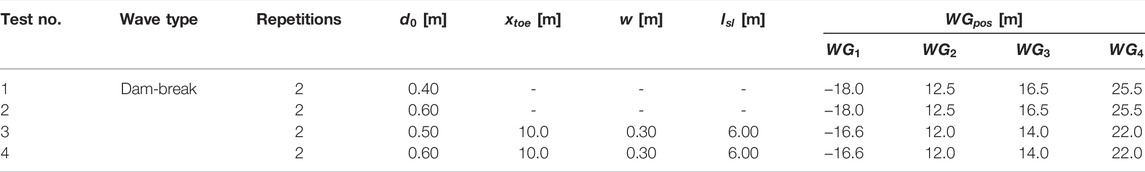
TABLE 1. Experimental protocol. Variables and coordinates correspond to Figure 2. Impoundment depth $d_0$, the distance between gate and toe of the slope $x_{toe}$, length of the slope $l_{sl}$, and height of the horizontal plane $w$. The positions of the wave gauges are given in the flume’s coordinates.

2.2 Calibration and Validation of the Numerical Model

Within this study, the software package REEF3D is used. REEF3D is an open-source hydrodynamics framework developed by Bihs et al. (2016), consisting of several numerical modules. The computational fluid dynamics (CFD) solver within REEF3D is used to solve the incompressible unsteady Reynolds-averaged Navier–Stokes (URANS) equations. This approach is selected since the flow is expected to be highly transient, which cannot be represented by the classical RANS formulation. The URANS approach can consider vortices in the front of the dam-break wave and is less costly in terms of computation compared to LES (large eddy simulation, see Iaccarino et al. (2003) for a comparison of the approaches). In addition to these CFD approaches, REEF3D is also used to solve depth-averaged non-hydrostatic shallow water equations (SWE) (Wang et al., 2020), which are much more computationally efficient than CFD calculations and are used by a multitude of authors to approximate dam-breaks; see Brufau and Garcia-Navarro (2000), Liang (2010), Ostapenko (2007), and Ozmen-Cagatay and Kocaman (2010). In order to identify the approach that represents the best compromise between efficiency and accuracy, URANS, SWE, and LES are compared against laboratory data of a flat bottom setup (test no. 1, see Table 1). This approach was chosen as the domain was still fairly large to be efficiently computed by the URANS approach. Figure 3 displays the time histories of the four wave gauges in comparison to the numerical approaches. Deviations in the measured time histories of the wave gauges are small in the reservoir (WG 1), where bottom friction almost does not influence the flow and no turbulences are present. The positive wavefront, however, propagating over the flumes’ bottom, results in larger deviations in the measurements. This is due to small imperfections in the flumes’ concrete bottom and a highly turbulent flow associated with large fluctuations. Calculations are performed on a regular grid with 0.01 m cell size in a two-dimensional domain and for a duration of 20 s (see Appendix 6.1 for a convergence study on cell size). The cell size represents the finest resolution, which leads to just acceptable long computing times (approx. 15 h per test in the numerical flume, see Section 2.3 and Appendix 6.1) on the available computing servers (two dual-socket CPU servers with AMD EPYC 7452; in total 128 cores at 2.35 GHz and 128 GB RAM) with the setting of the numerical model summarized in Appendix 6.2.

FIGURE 3

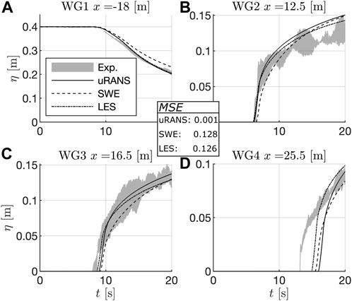
FIGURE 3. Comparison between three numerical approaches compared against experimental data of a dam-break wave propagating on a flat bottom (test no. 1, see Table 1). Four wave gauge time histories are displayed; one in the reservoir section (A) and three in the propagation section (B-D) of the flume. The mean squared errors (MSE) over all four time histories are given.

All approaches are in good agreement with the experimentally measured data. However, large eddy simulations are computationally costly, hence, the validation concentrates on the URANS and SWE approaches with the following settings (also summarized in Appendix 6.2, showing the control file of REEF3D): for the URANS approach, the WENO (weighted essentially non-oscillatory) scheme (Jiang and Shu, 1996) is used for the convection discretization and the level set method is used to track the free surface (Osher and Sethian, 1988). The scheme can handle large gradients accurately by taking smoothness into account, and it is deemed to be appropriate to handle wet front progress; it was confirmed to be accurate in simulating dam-break scenarios as well (Sun et al., 2012; Cannata et al., 2018; Li et al., 2020). Turbulence is approximated by using the $k-\omega$ turbulence model (Wilcox, 2006), where $k$ is the turbulent kinetic energy and $\omega$ is the specific turbulent dissipation. Time stepping for the momentum equation is performed by the TVD Runge–Kutta scheme, which is also applied to the level set and reinitialization method. The pressure is calculated using the projection method (Chorin, 1968). In the case of the SWE approach, the REEF3D:SFLOW implementation is used (Wang et al., 2020), which solves for non-hydrostatic pressure using a quadratic approximation (Jeschke et al., 2017) and uses the WENO scheme for convection. Figure 4 shows validation runs of the URANS and the SWE approach against wave gauge time histories of the experimental tests 2–4 (see Table 1). In analogy to Figure 3, the SWE approach shows good results compared to a larger dam-break wave on the horizontal bottom (test 2, see Table 1), cp. Figures 4A–D. However, once a composite bathymetry is modeled (Figure 4E-L), the SWE solution significantly underestimates the water depth along the slope (Figures 4F, G, J, K); it also overestimates the water depth on the adjacent horizontal plane (Figures 4H, L). The SWE cannot resolve vertical velocities, yet these would become relevant, especially where slope change occurs. Equally, these are also important to resolve reflection processes at and along the slope (see Section 3.2.1). However, the URANS approach is in good agreement with the experimental data and will hence be used within this study.

FIGURE 4

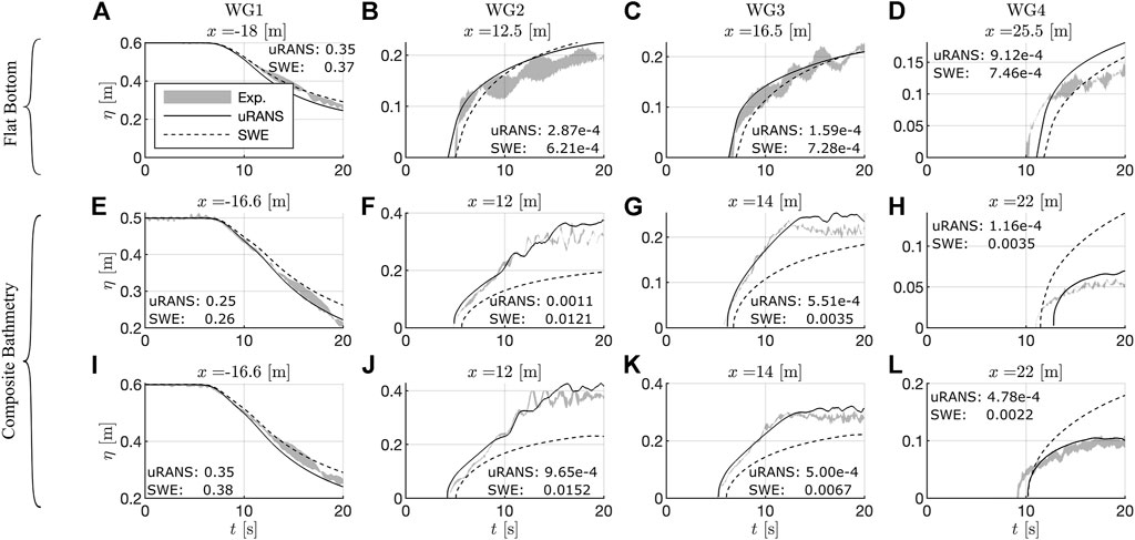
FIGURE 4. Numerically calculated wave gauge time histories (SWE and URANS approach) compared to laboratory data. Flat bottom test with initial impoundment depth ${\mathit{d}}_0=0.60$ m ((A–D), test no. 2, see Table 1), composite bathymetry with ${\mathit{d}}_0=0.50$ m ((E–H), test no. 3, see Table 1), and composite bathymetry with ${\mathit{d}}_0=0.60$ m ((I–L), test no. 4, see Table 1). Deviations between experimental and numerical data are given as MSE in each subfigure.

2.3 Numerical Flume and Test Protocol

The two-dimensional (2D) numerical flume (see Figure 5) consists of a solid bottom and left boundary, while the right boundary is an outflow to prevent reflections. The sides of the numerical flume are symmetry planes. The length of the reservoir $l_{res}$ equals the length of the propagation section ($l_{res}=x_{Toe}+l_{sl}+l_{hor}$). Since—theoretically and neglecting friction—the negative wavefront, propagating upstream in the reservoir section, is half the celerity of the positive wavefront, a reservoir length equal to the length of the propagation section minimizes the influences of an emptying reservoir on the hydrodynamics on the horizontal plane. The simulation time $t_{sim}$ is hence chosen to be twice the time the negative wavefront needs to reach the end of the flume and is, therefore, a function of the impoundment depth and the reservoir length and reads as follows:

${\mathit{t}}_{\mathit{sim}}=2\left({\mathit{l}}_{\mathit{res}}/\sqrt{\mathit{g}{\mathit{d}}_0}\right)\mathit{ }\left[\mathit{s}\right].(1)$

FIGURE 5

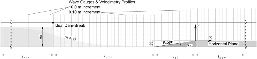
FIGURE 5. Side-view sketch of the numerical flume. Wave gauges and velocimetry profilers are placed over the entire domain with a spacing of $0.10\mathit{ }\mathbf{m}$ and $10.0\mathit{ }\mathbf{m}$. The free surface profile is indicated by $\mathit{\eta }$, the length of the reservoir ${\mathit{l}}_{\mathit{res}}$, the constant length of the horizontal plane ${\mathit{l}}_{\mathit{hor}}=10\mathit{ }\mathbf{m}$, the length ${\mathit{l}}_{\mathit{sl}}$ and the height $\mathit{w}$ of the slope, the distance between the initial water column and slope ${\mathit{x}}_{\mathit{Toe}}$, and the initial impoundment depth ${\mathit{d}}_0$.

The simulation time $t_{sim}$ can be converted into a dimensionless simulation time $T_{sim}$ in analogy to the expression from Wüthrich et al. (2018): $T=t\sqrt{g/d_0}$, so that the dimensionless simulation time $T_{sim}$ reads as follows:

${\mathit{T}}_{\mathit{sim}}=2{\mathit{l}}_{\mathit{res}}/{\mathit{d}}_0[-].(2)$

An ideal dam-break wave is ensured by an instantaneous release of the water column (starting with the first computational iteration, without simulating any gate). Wave gauges and velocimetry profilers, distributed over the entire domain with increments of 0.1 m in the propagation and 10 m in the reservoir section, yield spatio-temporal information about the flow features and the surface elevation. Simulations are performed on a regular grid with 0.01 m spacing using the URANS approach (see Section 2.2 for detailed settings and reasoning, as well as Appendix 6.2).

The geometry and the position of the composite bathymetry affect the hydrodynamics of the dam-break wave during propagation. To connect the parameters describing the composite bathymetry’s geometry with the hydrodynamics and the underlying physical processes, the parameters are systematically varied. Those parameters investigated in this work are (see Figure 5) the initial impoundment depth $d_0$, the distance between the initial water column and the toe of the slope $x_{toe}$, the length of the slope $l_{sl}$, and the height of the horizontal plane $w$. Three values are examined for each of these four parameters. This results in $3^4=81$ possible combinations of parameters or a number of tests, respectively. In addition, three reference tests with changing impoundment depth but a horizontal bottom (without composite bathymetry) are performed. Thus, in total, 84 tests are conducted. Table 2 lists the values of the four parameters being varied systematically ($d_0$, $x_{toe}$, $l_{sl}$, and $w$). In addition, the table contains the range of these values in dimensionless writing (indicated by capital letters: $X_{toe}$, $L_{sl}$, and $W$) normalized by the initial impoundment depth $d_0$ as commonly applied in studies on dam-break waves (Lauber and Hager, 1998; Chanson, 2009; Nouri et al., 2010; Oertel and Bung, 2012; Goseberg et al., 2013; Goseberg and Schlurmann, 2014; Hooshyaripor et al., 2017; von Häfen et al., 2018; Wüthrich et al., 2018; von Häfen et al., 2019; von Häfen et al., 2021).

TABLE 2

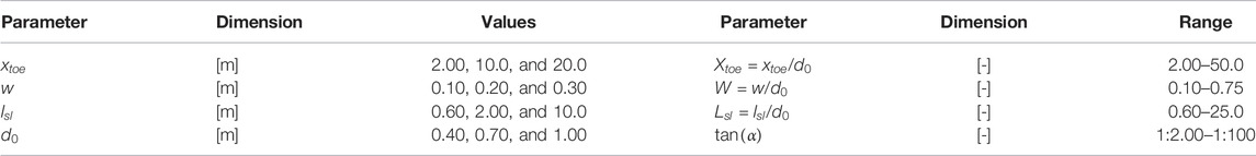
TABLE 2. Values of the parameters varied (left) and normalized parameter range (right).

3 Results

3.1 Flow Features over Space and Time–Analytical Considerations

The literature review revealed that in most experimental or numerical studies incorporating dam-break waves, there is little information on how the distance between the test setup and the (idealized) gate is chosen. However, dam-break waves’ hydrodynamics change considerably over space and time, which will be briefly highlighted in this section. Based on the analytical approach of Ritter (1897), Figures 6A–C show the computed surface elevation ($\eta$, panel A), depth-averaged flow velocity ($U$, panel B), and the Froude number ($F_r$, panel C) of a dam-break wave over space (abscissa) and time (ordinate). The dam-break location is at $x=0 \text{m}$, the reservoir extends into negative $x$-direction, whereas the propagation section is positive in $x$-direction. The positive wavefront is indicated as a red solid line, while the negative wave, propagating in opposite direction within the reservoir, is shown as a red dashed line.

FIGURE 6

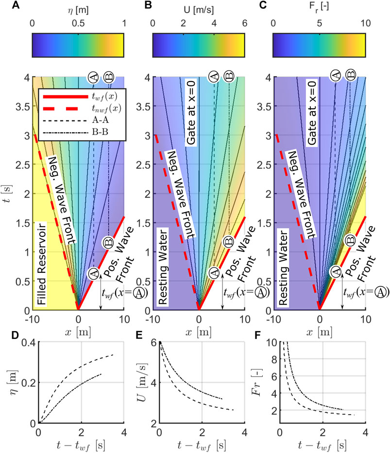
FIGURE 6. Flow features of a dam-break wave in space and time derived from the analytical approximation by Ritter (1897). Surface elevation (A), depth-averaged velocity (B), and Froude number (C) are indicated as colors. Dam-break location at x = 0 m, reservoir spreading in negative x-direction. Dry, frictionless propagation section on positive x-direction. Positive and negative wavefronts are indicated as solid and dashed red lines. These lines also indicate the time when the positive or negative wave reaches a specific position (${\mathit{t}}_{\mathit{wf}}$ and ${\mathit{t}}_{\mathit{nwf}}$, respectively). Isolines are displayed as thin black solid lines. Transects over time (A–A, B–B) are indicated in each subfigure (A–C) as dashed lines. Time histories at these transects are displayed in subfigures (D–F).

Figure 6 shows that surface elevation, velocity, and, subsequently, also the Froude number always depend on space and time. This is evident from the changing color gradients at constant x in Figures 6A–C and is emphasized in Figures 6D–F, which show the time series along the transects A and B, shifted to the time of positive wavefront arrival ($t_{wf}$). The larger the distance between the gate and the location being considered (e.g., the location of the test setup), the

1) lower and flatter the surface elevation time history (see Figure 6D),

2) higher the depth-averaged flow velocities over time (see Figure 6E), and

3) larger the Froude number time history (see Figure 6F).

Hence, the distance between the gate and test setup should preferably be provided in dam-break wave-structure interaction studies; this is to ensure comparability and repeatability of tests. In addition, the distance can be utilized to adjust the local hydrodynamic setting and to achieve conditions as close to in situ conditions as possible. Within the subsequently evaluated numerical test program, the distance between the gate and the toe of the slope ($x_{toe}$) is hence varied (see Table 2) to adjust for the gate to compound beach distance effect and to provide just comparisons.

Note that friction is neglected by the analytical approach of Ritter (1897). Even though the approach resembles the overall characteristics of a dam-break wave well, friction significantly influences the waves’ tip region (e.g., addressed by Chanson (2009)). Hence, close to the wave tip, the surface elevation will be larger and the depth-averaged velocities and Froude numbers smaller in nature than predicted by Ritter (1897) and presented in Figure 6.

3.2 Numerical Investigations

The following sections are using the computational results of the numerical model to investigate the flow features of the dam-break waves over compound bathymetries. First, some qualitative observations will be presented before flow depth and velocities as well as Froude numbers are investigated next.

3.2.1 Qualitative Observations

To introduce the data set of computed results with 84 individual tests, all of them with changing domain size, bottom profile, and impoundment depth, a qualitative analysis is performed first. The analysis is based on the velocity field (left column of Figure 7) and the turbulent kinetic energy (TKE, right column of Figure 7) in the x-z plane at two instants in time. The analysis first looks at the time $T\left(po{s}_{front}=9\text{m}\right)$, which is the instant in time when the wavefront reached the end of the computational domain, and afterward at the time $T=T_{sim}$ (see Eq. 2) representing the end of the computational time.

FIGURE 7

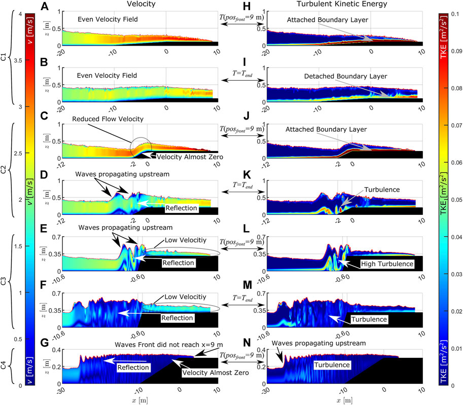
FIGURE 7. Velocity fields (left column) and turbulent kinetic energy (right columns) of classes C1–C4 (indicated by brackets on the left) at two instants in time (upper and lower row of each class) of class C1 (A,B,H,I), class C2 (C,D,J,K), class C3 (E,F,L,M), and class C4 (G,N). Velocities are given in bolt and the turbulent kinetic energy in ${\mathbf{m}}^2/{\mathbf{s}}^2$. The composite bathymetry is indicated as a black area.

Visual inspection of the surface elevation data along with the velocity fields and the TKE in the x-z plain has led to a classification of numerical test runs described hereafter in Table 3. The classification introduces four classes the authors identified (hereinafter referred to as classes C1 to C4), which are used in the subsequent data evaluation. Table 3 also indicated whether the surface elevation, front velocity, and Froude number of the classes are typically smaller or larger than the reference tests, where no composite bathymetry is present.

TABLE 3

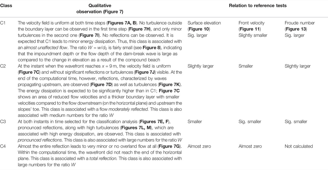
TABLE 3. Class definition and relation of flow features to reference tests.

Although the classification presented in Table 3 is qualitative at this point, the subsequent data analysis of each class presents a quantitative classification. However, since surface elevations, front velocities, and Froude numbers always depend on space, time, and the initial impoundment depth (A-C), no absolute values can be given per class in Table 3.

Looking at the flow visualizations mentioned earlier, it becomes clear that the complex two-dimensional flow patterns observed on the slope in classes C2–C4 cannot be represented well by a depth-averaged numerical approach, such as the shallow water wave equations (SWE). This explains the numerical results observed when validating the model (see Section 2.2); the SWE represented tests without a composite bathymetry were accurate and highly efficient in terms of computational time. However, once a composite bathymetry profile is installed, averaging over the water columns is an oversimplification as can be seen in Figure 7.

The remainder of this work uses a couple of definitions that are defined next. A “class” describes a group of tests showing similar hydrodynamics, as described earlier. ‘Class-averaged’ means that all data belonging to a class are averaged (eventually further subdivided into the different impoundment depths). The entire dataset of 81 tests is next classified into the previously defined classes. To link the geometrical parameters of the composite bathymetry with the previously identified classes (C1-C4, Figure 7), all tests are analyzed and displayed dimensionless in Figure 8.

FIGURE 8

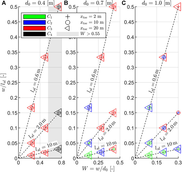
FIGURE 8. Dimensionless visualization of the observed classes in relation to the composite bathymetries’ parameters; slope steepness on the ordinate, dimensionless elevation of the horizontal plane (W) on the abscissa, and ${\mathit{x}}_{\mathit{toe}}$ indicated by markers and separated by initial impoundment depth(A-C). Dashed lines indicate tests with equal slope length. Classes are indicated by colors. Gray-shaded area covers W-values larger than $\sim$0.55 (only visible in (A)), which is found to be a delimitation criterion above which no overland flow is observed (class C4; total reflection).

The dimensionless abscissa of Figure 8 shows that for large impoundment depth (Figure 8C) and $W=0.3[-]$, classes C1–C3 are mostly observed, while for small impoundment depth (Figure 8A), only C3 classes occur, comparing the same $W$ -value. Thus, the smaller the impoundment depth, the more pronounced the reflections for the same dimensionless height $W$ of the horizontal plane. Taking the ordinate into account, which displays the dimensionless slope steepness, it is revealed that the steeper the slope (large $w/l_{sl}$ values), the more pronounced the occurrence of reflections (C2–C4 classes). Based on the findings presented in the previous section, an obvious relation between class occurrence and $x_{toe}$, represented by the triangle, circle, and plus signs, was expected. These symbols always lie on top of each other since each test is performed with each value of $x_{toe}$. A dependency on $x_{toe}$ would result in changing color coding of the signs laying on top of each other, however, this cannot be seen; a finding being discussed in Section 4. In conclusion, the more pronounced the reflections (increasing order of the class numbers):

1) the smaller the initial impoundment depth ($d_0$),

2) the larger the dimensionless height of the horizontal plane ($W)$, and

3) the steeper the slope ($w/l_{sl}$).

A dimensionless slope steepness larger than approximately $W\sim 0.55$ is found to be a delimitation criterion above which very minor to no overland flow is observed (class C4; total reflection).

3.2.2 Flow Depth on Horizontal Plane

After classifying the investigated tests, the flow conditions as a result of the dam-break waves are investigated next. To that end, the flow depth at the transition point between the slope and the upper horizontal elevation ($x=0 \text{m}$) is considered. Figure 9 shows the class-averaged surface elevation time histories at this position. They are normalized over the initial impoundment depth ($d_0$) and displayed over the dimensionless time ($T=t\sqrt{g/d_0}$) for each impoundment depth separately. Classes are indicated as colored areas which extend plus-minus the standard deviation ($\sigma$) above and below the class-averaged time-histories $\left(\overline{\eta /d_0}\right)$. Lines (solid, dashed, and dotted) represent approximations of the time histories. Coefficients of determination ($r^2$) between time histories and approximations are given.

FIGURE 9

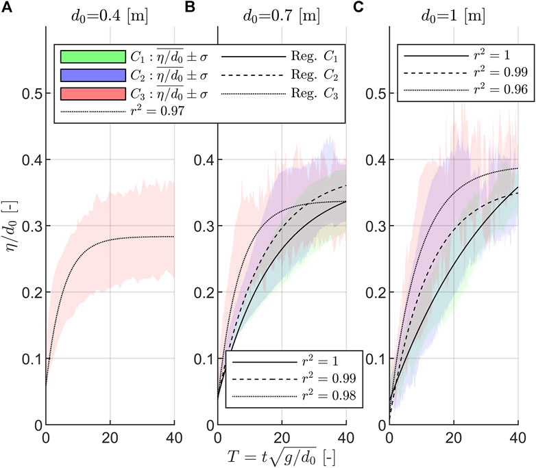
FIGURE 9. Class-averaged normalized surface elevation time history ($\mathit{\eta }/{\mathit{d}}_0$, on the ordinate) separated by classes (C1–C3) at the transition point ($\mathit{x}=0\mathit{ }\mathbf{m}$) over dimensionless time ($\mathit{T}=\mathit{t}\sqrt{\mathit{g}/{\mathit{d}}_0}$) and separated by initial impoundment depth (A–C). Colored areas represent class-averaged surface elevation time history plus-minus the standard deviation. Lines represent an approximation following Eq. 3. Coefficients of determination (${\mathit{r}}^2$) between time histories and approximations are given.

Figure 9 shows a dependency of the dimensionless class-averaged surface elevation time-histories on the initial impoundment depth; the larger the initial impoundment depth, the larger the dimensionless flow depth. This observation reveals that flow depth at the transition point is disproportional to the initial impoundment depth. However, it is common practice to normalize the flow depth of a dam-break wave over the initial impoundment depth (see e.g., Lauber and Hager, 1998; Chanson, 2009; Nouri et al., 2010; Oertel and Bung, 2012; Goseberg et al., 2013; Goseberg and Schlurmann, 2014; Hooshyaripor et al., 2017; von Häfen et al., 2018; Wüthrich et al., 2018; von Häfen et al., 2019; von Häfen et al., 2021). This observation is being discussed further in Section 4. Considering the classes C1–C3, it becomes apparent that C3 (pronounced reflections) leads to a steeper increasing surface elevation time history than C2 (medium reflections) or C1 (minor/no reflections) (see Figure 9B or Figure 9C). Thus, the more dominant the reflections in the run-up/overland flow evolution, the faster the surface elevation increases at the beginning of the time histories. Tests associated with pronounced reflections (C3) also lead to larger flow depth than C2 or C1. In addition, the larger the standard deviation, the more pronounced the reflection. To predict the class-averaged surface elevation time history, an approximation is fitted to the data, which is a function of the initial impoundment depth, the dimensionless time, and the class, that follows the form of Eq. 3 with the coefficients $(a-g)$ given in Table 4. Eq. 3 is an exponential function over dimensionless time with a linear dependency on the initial impoundment depth, and it reads as follows:

$\frac{\mathit{\eta }}{\mathit{d}0}\left({\mathit{d}}_0,\mathit{T},\mathit{C}\right)=\left\{\mathit{a}{\mathit{d}}_0+\mathit{b}\right\}{\mathit{e}}^{-\left\{\mathit{c }{\mathit{d}}_0+\mathit{d}\right\}\mathit{T}}+\left\{\mathit{f}{\mathit{d}}_0+\mathit{g}\right\}[-].(3)$

TABLE 4

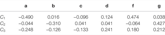
TABLE 4. Coefficients to Eq. 3.

To obtain information about the class-averaged surface elevation over the entire length of the horizontal plane, surface elevation lines ($\eta$ over space, referred to as SEL) are calculated at three instants in time. The surface elevation lines are normalized using the reference tests (${\eta }_{ref}$, plain horizontal bottom, no composite bathymetry present) as displayed in Figure 10.

FIGURE 10

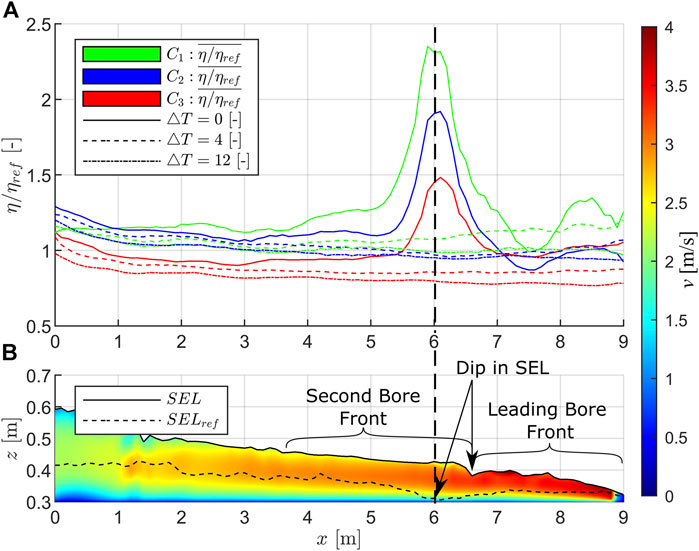
FIGURE 10. Visualization of class-averaged surface elevation lines (SELs) over space (A). Classes are indicated by color and instants in time by line type. Local flow velocities (B) are color coded according to the color bar, Reference SEL by a dashed line. Dimensionless time steps $\Delta \mathit{T}$ describe the additional time after wavefront first reached the end of the horizontal plane at $\mathit{x}=9\mathit{ }\mathbf{m}$.

Figure 10A shows SELs for three dimensionless instants in time; the instant when the wavefront reaches the end of the horizontal plane and two later ones (plus $\Delta T=4$ and $\Delta T=12$). The following can be extracted from Figure 10A:

1) Independent of time and space, tests associated with minor reflections and turbulences (C1) show overall larger normalized flow depths than those tests with more pronounced reflections (C2 and C3).

2) Class C3 shows smaller flow depths than the reference tests. This is due to the significant energy dissipation and reflection associated with this class. Class C2 shows normalized flow depths close to one (except for the peaks at $x=6 \text{m}$), while C1 shows the largest normalized flow depth.

3) Close to the transition point ($x=0 \text{m}$), larger class-averaged normalized flow depths are observed than further downstream (except for the peaks at $x=6 \text{m}$). This is due to the inertia of the flow coming from the slope and evolving over the slope transition into the horizontal plane. This leads to a change in flow direction at the transition point, which is associated with forces (gravity in this case) acting on the flow.

4) Thus, the stronger the effect is, the more pronounced the change in flow direction in relation to flow velocity is. Therefore, this effect is more pronounced for C3 (pronounced reflections due to steep and high slopes, see Figure 8 for class occurrence with respect to the slope parameters) than for C2. For C1, almost no change in flow depth at the transition point is observed.

Peaks are observed in the class-averaged dimensionless SEL for all classes (C1–C3) and for $\Delta T=0$. Figure 10B reveals the cause of the peaks’ occurrence; in some tests, a leading bore front is observed in the surface elevation (solid line in Figure 10B) and in the reference SEL too. The dashed vertical line in Figure 10 indicates that small surface elevation in the reference class ($SE{L}_{ref}$) occurs simultaneously with large surface elevation in the concerned tests, leading to the peaks in the normalized surface elevation in Figure 10A. This phenomenon, which is discussed in Section 5, is typical for dam-break waves. Therefore, velocity time histories are not displayed, but median velocities over space normalized by the velocity of the corresponding reference tests $\left(c_{ref}\right)$ are provided in Figure 11.

FIGURE 11

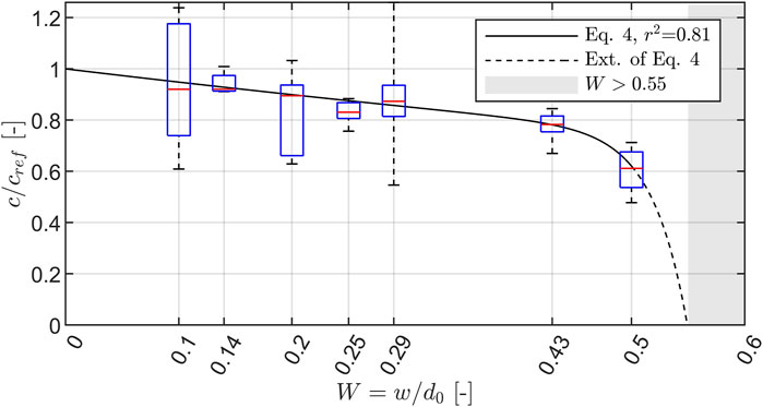
FIGURE 11. Bore front velocities $\left(\mathit{c}\right)$ normalized over the corresponding reference front velocities (${\mathit{c}}_{\mathit{ref}}$, no compound beach present) and averaged over space using the median. Data are plotted over the height of the horizontal plane normalized over the initial impoundment depth ($\mathit{W}=\mathit{w}/{\mathit{d}}_0$). Boxplots are defined as follows: the median is indicated as a red bar, and the box indicates the 75th and 25th percentile, respectively. Whiskers extend to the most extreme data points. The black solid line represents the approximation given by Eq. 4. The dashed line indicates the extrapolation of Eq. 4. Gray-shaded area covers values of W larger than 0.55, where no overland flow is observed.

Figure 11 covers all front velocities for tests belonging to C1–C3, and C4 (almost the entire reflection) is excluded as almost no overland flow occurred in this class. The following can be extracted from the data analysis and Figure 11:

1) The higher the horizontal plane, the lower the front velocity. This observation is plausible since the larger the height of the horizontal plane, the more pronounced the reflections, and thus the energy dissipation increases considerably.

2) The median $c/c_{ref}$ - values are always smaller than unity. The median wavefront velocity is slower than the corresponding reference. Due to energy dissipation on the composite bathymetry, which is not present in the reference class, this observation is plausible too.

3) In contrast to all other data points, the data for the smallest dimensionless height of the horizontal plane ($w/d_0 =0.1$) shows a 75th percentile larger than one, indicating that the wavefront is moving faster than the reference class. This phenomenon can be explained by a fast-moving leading bore front (see Figure 10B) observed in many of these tests.

4) The decreasing trend, indicated by the black solid line, is almost linear up to $W=0.43$. For larger values, the front velocity, however, rapidly decreases. The linear trend is due to the fact that the larger the normalized height of the horizontal plane, the more pronounced the reflections. The rapid decrease for values beyond $W=0.43$ is caused by almost the entire energy being dissipated at the slope. In line with the qualitative observations (see Figure 8), total reflections and consequently front velocities of zero are expected for values larger than $W \sim 0.55$.

The approximation and its extrapolation, to be seen in Figure 11, read as follows:

$\frac{\mathit{c}}{{\mathit{c}}_{\mathit{ref}}}={\mathit{e}}^{-0.53\left(\mathit{w}/{\mathit{d}}_0\right)}-{10}^{-8}{\mathit{e}}^{33\left(\mathit{w}/{\mathit{d}}_0\right)}[-],(4)$

where c is the front velocity of the overland flow, $c_{ref}$ is the front velocity of the reference class at the same longitudinal distance to the waves’ origin, w is the height of the horizontal plane, and $d_0$ is the initial impoundment depth. The approximation correlates well with the median values (red bars in Figure 11, $r^2=0.81$).

3.2.3 Froude Number on Horizontal Plane

The dimensionless Froude number can be calculated based on the flow velocity and the corresponding water depth at a certain position over time and is frequently reported in studies about post-tsunami surveys (e.g., Fritz et al., 2006b). In Figures 12G and H, the depth-averaged Froude number at the transition point ($x=0 \text{m}$) over dimensionless time is displayed beside the corresponding surface elevation time histories (Figures 12A–C) and depth-averaged flow velocities (Figures 12D–F) separated by initial impoundment depth and class. Reference time histories are extracted from the reference tests for each considered test using the same distance between the idealized gate and transition point (since hydrodynamics change over space, as presented in Section 3.1). All time histories displayed in Figure 12 are class averaged.

FIGURE 12

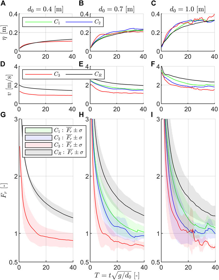
FIGURE 12. Visualization of class-averaged surface elevation ($\mathit{\eta }$, (A–C)), depth- and class-averaged velocity (v, (D–F)), and class-averaged Froude number (Fr, (F–I)) at the transition point over dimensionless time and separated by initial impoundment depth (${\mathit{d}}_0$). Standard deviation (2 $\mathit{\sigma }$) is displayed as a shaded area.

Figures 12A–C show that flow depths at the transition point are similar to the reference tests without a composite bathymetry present. Figures 12D–F, however, reveal flow velocities significantly smaller than the reference. The more pronounced the reflections (higher class number), the lower the depth-averaged flow velocities. In general, all velocity time histories show higher values at the beginning and decrease over time. The following can be extracted from Figures 12G–I displaying the Froude time histories:

1) In the first instant, very large Froude numbers are observed, rapidly decreasing over time. These high values are typical for dam-break waves and are due to the small flow depths combined with the large flow velocities in the wavefront.

2) The Froude numbers at the transition point of a composite bathymetry are generally smaller compared to those without such a bottom profile.

3) The more pronounced the reflections (thus, the higher the class number), the smaller the Froude numbers. This is caused by the flow velocities showing the same trend.

4) Class C3 shows, for later instants, Froude numbers smaller than one. Thus, the flow changes from super to subcritical.

To obtain spatial information about Froude numbers on the horizontal plane, three dimensionless instants in time $\Delta T$ after wavefront arrival at $x=9 \text{m}$ (end of the horizontal plane) are selected with $\Delta T=\left[4, 8, 12\right]$. Figure 13 displays class-averaged Froude numbers over space (indicated as thin, colored lines) and the reference tests. A multilinear approximation as given by Eq. 5 is indicated in wide, transparent lines.

FIGURE 13

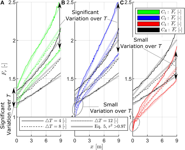
FIGURE 13. Visualization of class-averaged Froude numbers (thin lines) over space (at the horizontal plane) at three dimensionless instants in time $\Delta \mathit{T}=\left[\mathrm{4,8,12}\right]$. Data are displayed separately per class (A–C). The multilinear approximation is displayed as wide transparent lines.

The following findings can be extracted from Figure 13:

1) Froude numbers are independent of space, the smaller the Froude numbers are, the more pronounced the reflections (higher class numbers) are.

2) Class C3 (pronounced reflections) shows overall smaller Froude numbers than the reference, while for the classes with no and minor reflections (C1 and C2), Froude numbers are, except for the transition point at $x=0 \text{m}$, always larger than the reference.

3) The Froude numbers rise over space; this is typical for dam-break waves showing the largest Froude numbers in the wavefront region, decreasing downstream, where water depth increases and flow velocities decrease.

4) The Froude numbers show an almost linear trend over space; the more pronounced the linear trend, the smaller the influences of the composite bathymetry. However, the reference class shows the weakest linear trend; especially for $\Delta T=4$, the linear approximation underestimates the reference class at $x=0 \text{m}$ and $x=9 \text{m}$. This can be explained as follows: for large x-values, the approximation underestimates all Froude numbers. For small x-values, the approximation underestimates the reference class significantly, while the composite bathymetry tests are slightly overestimated. This is due to the transition point lowering the Froude numbers here.

5) The differences between the Froude numbers at the transition point differ from class to class; while the reference and C1 (Figure 13A) show a significantly changing Froude number over time at $x=0 \text{m}$ (in the same order of magnitude of the reference class); tests with more pronounced (C2) and significant reflection (C3) show a small variation in Froude number at the transition point over time. This is probably due to the strong turbulence on the slope associated with classes C2 and C3, partially interrupting the original hydrodynamics of the dam-break wave. This is indicated by the flow velocity at the transition point being significantly reduced compared to the reference tests (see Figures 12D–F).

6) Over space, the differences in Froude numbers increase over time. Thus, the largest variations in Froude number over time are observed at $x=9 \text{m}$.

The approximation displayed in Figure 13 is a multilinear function over space and dimensionless time. It is determined individually per class, yields a high coefficient of determination of $r^2>0.97$, and reads as follows:

${\mathit{F}}_{\mathit{r}}\left(\mathit{x},\mathit{T},\mathit{C}\right)=\left\{\mathit{a}\mathit{T}+\mathit{b}\right\}\mathit{x}+\left\{\mathit{c}\mathit{T}+\mathit{d}\right\}[-].(5)$

Coefficients in Eq. 5 are given in Table 5.

TABLE 5

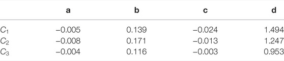
TABLE 5. Coefficients to Eq. 5.

4 Discussion

It was observed that the class occurrence (Figure 8) as well as the normalized flow depth at the transition point (Figure 9) change with changing initial impoundment depth $d_0$, even though the data are normalized over the initial impoundment depth, which is a common normalization. This phenomenon is unexpected since a dam-break wave is driven by gravity only and its energy/momentum is correlated with the initial impoundment depth. Theoretically, the larger the impoundment depth, the larger the ability to overcome a certain elevation (height of the horizontal plane). However, this study, which evaluates a large data set and focuses on the flow features on the horizontal plane, does not cover the complex processes on the slope. It is expected that vortex patterns, interactions of the incoming and reflected wave energy as well as the associated energy dissipation over the slope highly depend on the slope geometry and the initial impoundment depth, and that dam-break waves of smaller impoundment depth are more strongly affected by these effects.

As shown in Section 3.1, the distance between the gate and the place under consideration $x_{toe}$ (e.g., the position of test setup in a flume) must be considered since the hydrodynamics of a dam-break wave change over space. Therefore, a clear dependency between $x_{toe}$ and the class number (Figure 8) was originally expected but was not found. It is assumed that the turbulence on the slope disturbs the hydrodynamics of the dam-break wave to such an extent that these effects override the influence of $x_{toe}$.

Instead of a single leading bore front, in some classes, sequences of bores riding on top or next to each other were observed (see Figure 10). This phenomenon appears for both, the reference tests and the tests with composite bathymetries, but only at a distance of approximately 20 m downstream of the idealized gate and only for tests with an initial impoundment depth of 1 m. The formation of the leading bore is either an effect of the collapsing water column (like observed by Lauber (1997)) once the dam-break is initiated or due to disintegration of the wave while propagating. However, this study focuses on the flow features on the horizontal plane of the composite bathymetry, and thus this phenomenon is beyond the study’s scope. Further research is required to investigate the observed phenomenon.

Wall and bottom roughness are not varied within the study but set to a fixed equivalent sand roughness of $k_s=0.001$, representing a smooth surface. This roughness value compares well to the smooth surface of the composite bathymetry used in the physical tests and is a conservative assumption for the numerical parameter study since it leads to little friction and thus to large Froude numbers. Systematically varying the roughness with also three values (as performed for $d_0$, $x_{toe}$, $w$, and $l_{sl}$) would have increased the number of tests in the parameter study from 81 to 243 combinations. This would have tripled the computational time for the entire data set (from 50 days to about half a year), which would not have been possible within the scope of this study. However, it is expected that the bottom roughness influences the features of the overland flow, and hence future research should deepen research on this topic.

Froude numbers are found to be always larger than unity in the experiments, except for class C3 close to the transition point ($x=0 \text{m}$ in Figure 13C). In general, the larger the class order, the lower the Froude numbers. However, Fritz et al. (2006b) have reported that Froude numbers were close to unity during the 2004 Indian Ocean tsunami. Thus, even though a composite bathymetry can reduce Froude numbers in the experiment, the bathymetry profile alone is not enough to reach fully matching Froude numbers. It is expected that roughness elements (like the build environment) and debris lead to the lower Froude number observed by Fritz et al. (2006b). Generally, for both numerical and physical tests, Froude numbers should always be measured and test results qualified in terms of their comparability to real tsunami events.

The dimensionless ratio of the height of the horizontal plane to the initial impoundment depth $W\sim 0.55$ is found to be a delimitation criterion. For W values larger than approximately 0.55, only class C4 was observed and thus almost total reflection of the wave and only a little water on the horizontal plane. The wavefront did not reach the end of the computational domain within the simulation time. Shen and Meyer (1963) investigated the run-up of dam-break waves on a sloping bathymetry and found the following relationship:

$\mathit{R}={\mathit{U}}^2/\left(2\mathit{g}\right).(6)$

Equation 6 is based on the nonlinear shallow water equation, where R is the run-up height and U is the velocity on the slope toe. This relationship yields a dimensionless run-up height of $R/d_0\sim 0.3$ for $U\left(d_0=0.4 \text{m}\right)\sim 1.5 \text{m}/\text{s}$ observed in this study, being much smaller than the delimitation criterion $W=w/d_0\sim 0.55$. However, as mentioned by Lu and Liu (2017), Eq. 6 underestimates the run-up due to simplifications made by the shallow water equation, which is not capable of representing the flow features as observed in Section 2.2. Even though more refined approximations exist, they are not applicable to the present dataset due to using different boundary conditions (like an initially wet flume and limited reservoir length in Barranco and Liu (2021)) or waves (breaking dam-break waves used by Lu et al. (2018)) or bores (resulting from solitary waves used by Jensen et al. (2003)). The delimitation criterion found here should be verified in future work as well.

5 Conclusion

This study utilizes large-scale physical flume tests to validate and calibrate a numerical, two-dimensional CFD model. The numerical model is then used to investigate the flow features of a dam-break wave swashing over a composite bathymetry. Therefore, a parameter study is conducted altering all parameters influencing the dam-break waves’ hydrodynamics and the geometry of the composite bathymetry. The study focuses on the flow features observed on the horizontal plane in analogy to an urbanized site inundated by a tsunami propagating over a sloping bathymetry. The following findings are obtained and justified by data:

1) Classes are first proposed based on a qualitative rating system to distinguish between typical flow patterns based on visual inspection, which allows an assessment of the degree of reflection or energy dissipation due to the bathymetry profile.

2) These classes are correlated with the parameters systematically altered within the parameter study. This allows for predicting the class that will occur within the investigated parameter range. In addition, the typical flow features associated with a class are related to reference tests, where no composite bathymetry is present.

3) Flow features observed and associated with a class are described quantitatively (flow depth, velocity, and Froude number) over space and time, and the observations are linked to the underlying physical processes.

4) Empirical equations for the flow depth, velocity, and Froude number are presented based on the proposed classes and hence provide an approximate prediction for each test investigated. It is found that the flow features on the horizontal plane are governed by the (dimensionless) height of the horizontal plane and the initial impoundment depth. The slope angle and the distance between dam-break initiation and the toe of the slope are of minor importance.

5) Apart from the parameter study, simple and basic analytical considerations are made to display the changing hydromechanics of a dam-break wave over space and time. Therefore, the distance between dam-break initiation and test setup should always be given and, ideally, also justified.

The findings and approximations presented in this study first allow for predicting the flow regime on the horizontal plane of a composite bathymetry and, therefore, provide an approximate design tool for laboratory testing and significantly gain process understanding of real-world tsunami inundations.

Data Availability Statement

The raw data supporting the conclusions of this article will be made available by the authors, without undue reservation.

Author Contributions

HvH, HB, and NG contributed to the conceptualization. HvH, CK, HB, and NG developed the methodology. HvH carried out the numerical simulations, with the supervision of HB and NG. HvH wrote the first draft of the manuscript and prepared the visualizations. HB and NG provided supervision. NG is responsible for project administration and funding acquisition. All authors contributed to manuscript revision and read and approved the submitted version.

Funding

The support of the Volkswagen Foundation (project ‘Beyond Rigidity-Collapsing Structures in Experimental Hydraulics’, No. 93826) through a grant held by NG is greatly acknowledged. We acknowledge support by the Open Access Publication Funds of Technische Universität Braunschweig.

Conflict of Interest

The authors declare that the research was conducted in the absence of any commercial or financial relationships that could be construed as a potential conflict of interest.

Publisher’s Note

All claims expressed in this article are solely those of the authors and do not necessarily represent those of their affiliated organizations, or those of the publisher, the editors, and the reviewers. Any product that may be evaluated in this article, or claim that may be made by its manufacturer, is not guaranteed or endorsed by the publisher.

References

Ablain, M., Dorandeu, J., le Traon, P.-Y., and Sladen, A. (2006). High Resolution Altimetry Reveals New Characteristics of the December 2004 Indian Ocean Tsunami. Geophys. Res. Lett. 33 (21), 1–6. doi:10.1029/2006GL027533

CrossRef Full Text | Google Scholar

Al-Faesly, T., Palermo, D., Nistor, I., and Cornett, A. (2012). Experimental Modeling of Extreme Hydrodynamic Forces on Structural Models. Int. J. Prot. Struct. 3 (4), 477–505. doi:10.1260/2041-4196.3.4.477

CrossRef Full Text | Google Scholar

Aránguiz, R., Esteban, M., Takagi, H., Mikami, T., Takabatake, T., Gómez, M., et al. (2020). The 2018 Sulawesi Tsunami in Palu City as a Result of Several Landslides and Coseismic Tsunamis. Coast. Eng. J. 62 (4), 445–459. doi:10.1080/21664250.2020.1780719

CrossRef Full Text | Google Scholar

Arnason, H., Petroff, C., and Yeh, H. (2009). Tsunami Bore Impingement onto a Vertical Column. J. Disaster Res. 4, 391–403. doi:10.20965/jdr.2009.p0391

CrossRef Full Text | Google Scholar

Aureli, F., Dazzi, S., Maranzoni, A., Mignosa, P., and Vacondio, R. (2015). Experimental and Numerical Evaluation of the Force Due to the Impact of a Dam-Break Wave on a Structure. Adv. Water Resour. 76, 29–42. doi:10.1016/j.advwatres.2014.11.009

CrossRef Full Text | Google Scholar

Bihs, H., Kamath, A., Alagan Chella, M., Aggarwal, A., and Arntsen, Ø. A. (2016). A New Level Set Numerical Wave Tank with Improved Density Interpolation for Complex Wave Hydrodynamics. Comput. Fluids 140, 191–208. doi:10.1016/j.compfluid.2016.09.012

CrossRef Full Text | Google Scholar

Barranco, I., and Liu, P. L.-F. (2021). Run-up and Inundation Generated by Non-Decaying Dam-Break Bores on a Planar Beach. J. Fluid Mech. 915, A81. doi:10.1017/jfm.2021.98

CrossRef Full Text | Google Scholar

Bernard, E., and Titov, V. (2015). Evolution of Tsunami Warning Systems and Products. Phil. Trans. R. Soc. A 373 (2053), 20140371. doi:10.1098/rsta.2014.0371

PubMed Abstract | CrossRef Full Text | Google Scholar

Borrero, J. C., Synolakis, C. E., and Fritz, H. (2006). Northern Sumatra Field Survey after the December 2004 Great Sumatra Earthquake and Indian Ocean Tsunami. Earthq. Spectra 22, 93–104. doi:10.1193/1.2206793

CrossRef Full Text | Google Scholar

Brufau, P., and Garcia-Navarro, P. (2000). Two-Dimensional Dam Break Flow Simulation. Int. J. Numer. Meth. Fluids 33 (1), 35–57. doi:10.1002/(sici)1097-0363(20000515)33:1<35::aid-fld999>3.0.co;2-d

CrossRef Full Text | Google Scholar

Cannata, G., Petrelli, C., Barsi, L., Fratello, F., and Gallerano, F. (2018). A Dam-Break Flood Simulation Model in Curvilinear Coordinates. WSEAS Trans. Fluid Mech. 13, 60–70.

Google Scholar

Chan, I.-C., and Liu, P. L.-F. (2012). On the runup of Long Waves on a Plane Beach. J. Geophys. Res. Oceans 117 (8), 8006. Available at: https://www.scopus.com/inward/record.uri?eid=2-s2.0-84864859069&doi=10.1029%2f2012JC007994&partnerID=40&md5=ccce87da3709e91f78a82acef4b9ca81. doi:10.1029/2012jc007994

CrossRef Full Text | Google Scholar

Chanson, H. (2009). Application of the Method of Characteristics to the Dam Break Wave Problem. J. Hydraulic Res. 47 (1), 41–49. doi:10.3826/jhr.2009.2865

CrossRef Full Text | Google Scholar

Chanson, H. (2006). Tsunami Surges on Dry Coastal Plains: Application of Dam Break Wave Equations. Coast. Eng. J. 48 (4), 355–370. doi:10.1142/S0578563406001477

CrossRef Full Text | Google Scholar

Chock, G., Carden, L., Robertson, I., Olsen, M., and Yu, G. (2013). Tohoku Tsunami-Induced Building Failure Analysis with Implications for U.S. Tsunami and Seismic Design Codes. Earthq. Spectra 29, 99–126. doi:10.1193/1.4000113

CrossRef Full Text | Google Scholar

Chorin, A. J. (1968). Numerical Solution of the Navier-Stokes Equations. Math. Comp. 22 (104), 745–762. doi:10.2307/200457510.1090/s0025-5718-1968-0242392-2

CrossRef Full Text | Google Scholar

Cross, R. H. (1967). Tsunami Surge Forces. J. Wtrwy. Harb. Div. 93, 201–231. doi:10.1061/jwheau.0000528

CrossRef Full Text | Google Scholar

Derschum, C., Nistor, I., Stolle, J., and Goseberg, N. (2018). Debris Impact under Extreme Hydrodynamic Conditions Part 1: Hydrodynamics and Impact Geometry. Coast. Eng. 141, 24–35. doi:10.1016/j.coastaleng.2018.08.016

CrossRef Full Text | Google Scholar

Dressler, R. F. (1952). Hydraulic resistance Effect upon the Dam-Break Functions. J. Res. Natl. Bur. Stan. 49, 217. doi:10.6028/jres.049.021

CrossRef Full Text | Google Scholar

Dressler, R. F., and Stoneley, R. (1958). Unsteady Non-Linear Waves in Sloping Channels. Proc. R. Soc. Lond. A 247 (1249), 186–198. doi:10.1098/rspa.1958.0177

CrossRef Full Text | Google Scholar

Farahmandpour, O., Marsono, A. K., Forouzani, P., Md Tap, M., and Abu Bakar, S. (2020). Experimental Simulation of Tsunami Surge and its Interaction with Coastal Structure. Int. J. Prot. Struct. 11 (2), 258–280. doi:10.1177/2041419619874082

CrossRef Full Text | Google Scholar

Fernandez-Feria, R. (2006). Dam-Break Flow for Arbitrary Slopes of the Bottom. J. Eng. Math. 54 (4), 319–331. doi:10.1007/s10665-006-9034-5

CrossRef Full Text | Google Scholar

Fritz, H. M., Borrero, J. C., Synolakis, C. E., and Yoo, J. (2006b). 2004 Indian Ocean Tsunami Flow Velocity Measurements from Survivor Videos. Geophys. Res. Lett. 33 (24), 1–5. doi:10.1029/2006GL026784

CrossRef Full Text | Google Scholar

Fritz, H. M., Petroff, C. M., Catalán, P. A., Cienfuegos, R., Winckler, P., Kalligeris, N., et al. (2011). Field Survey of the 27 February 2010 Chile Tsunami. Pure Appl. Geophys. 168 (11), 1989–2010. doi:10.1007/s00024-011-0283-5

CrossRef Full Text | Google Scholar

Fritz, H. M., Phillips, D. A., Okayasu, A., Shimozono, T., Liu, H., Mohammed, F., et al. (2012). The 2011 Japan Tsunami Current Velocity Measurements from Survivor Videos at Kesennuma Bay Using LiDAR. Geophys. Res. Lett. 39 (7), 1–6. doi:10.1029/2011GL050686

CrossRef Full Text | Google Scholar

Fritz, H. M., Synolakis, C. E., and McAdoo, B. G. (2006a). Maldives Field Survey after the December 2004 Indian Ocean Tsunami. Earthq. Spectra 22, 137–154. doi:10.1193/1.2201973

CrossRef Full Text | Google Scholar

Ghobarah, A., Saatcioglu, M., and Nistor, I. (2006). The Impact of the 26 December 2004 Earthquake and Tsunami on Structures and Infrastructure. Eng. Struct. 28 (2), 312–326. doi:10.1016/j.engstruct.2005.09.028

CrossRef Full Text | Google Scholar

Ghodoosipour, B., Stolle, J., Nistor, I., Mohammadian, A., and Goseberg, N. (2019). Experimental Study on Extreme Hydrodynamic Loading on Pipelines Part 2: Induced Force Analysis. J. Mar. Sci. Eng. 7 (8), 262. doi:10.3390/jmse7080262

CrossRef Full Text | Google Scholar

Goff, J., Liu, P. L.-F., Higman, B., Morton, R., Jaffe, B. E., Fernando, H., et al. (2006). Sri Lanka Field Survey after the December 2004 Indian Ocean Tsunami. Earthq. Spectra 22, 155–172. doi:10.1193/1.2205897

CrossRef Full Text | Google Scholar

Goseberg, N., and Schlurmann, T. (2014). “Non-Stationary Flow Around Buildings during run-Up of Tsunami Waves on a Plain Beach,” in Proceedings of the Coastal Engineering Conference, Seoul, Republic of Korea, 2014-January. https://www.scopus.com/inward/record.uri?eid=2-s2.0-84957625748&partnerID=40&md5=4bfcf145c56fef3f5cf81766453d6f77. doi:10.9753/icce.v34.currents.21

CrossRef Full Text | Google Scholar

Goseberg, N., Wurpts, A., and Schlurmann, T. (2013). Laboratory-Scale Generation of Tsunami and Long Waves. Coast. Eng. 79, 57–74. doi:10.1016/j.coastaleng.2013.04.006

CrossRef Full Text | Google Scholar

Grue, J., Pelinovsky, E. N., Fructus, D., Talipova, T., and Kharif, C. (2008). Formation of Undular Bores and Solitary Waves in the Strait of Malacca Caused by the 26 December 2004 Indian Ocean Tsunami. J. Geophys. Res. 113 (C5), 1–14. doi:10.1029/2007JC004343

CrossRef Full Text | Google Scholar

Hooshyaripor, F., Tahershamsi, A., and Razi, S. (2017). Dam Break Flood Wave under Different Reservoir's Capacities and Lengths. Sādhanā 42 (9), 1557–1569. doi:10.1007/s12046-017-0693-x

CrossRef Full Text | Google Scholar

Hunt, B. (1983). Asymptotic Solution for Dam Break on Sloping Channel. J. Hydraul. Eng. 109 (12), 1698–1706. doi:10.1061/(asce)0733-9429(1983)109:12(1698)

CrossRef Full Text | Google Scholar

Hunt, B. (1984). Perturbation Solution for Dam‐Break Floods. J. Hydraul. Eng. 110 (8), 1058–1071. doi:10.1061/(asce)0733-9429(1984)110:8(1058)

CrossRef Full Text | Google Scholar

Iaccarino, G., Ooi, A., Durbin, P. A., and Behnia, M. (2003). Reynolds Averaged Simulation of Unsteady Separated Flow. Int. J. Heat Fluid Flow 24 (2), 147–156. doi:10.1016/S0142-727X(02)00210-2

CrossRef Full Text | Google Scholar

Jaffe, B. E., Borrero, J. C., Prasetya, G. S., Peters, R., McAdoo, B., Gelfenbaum, G., et al. (2006). Northwest Sumatra and Offshore Islands Field Survey after the December 2004 Indian Ocean Tsunami. Earthq. Spectra 22, 105–135. doi:10.1193/1.2207724

CrossRef Full Text | Google Scholar

Jensen, A., Pedersen, G. K., and Wood, D. J. (2003). An Experimental Study of Wave run-Up at a Steep Beach. J. Fluid Mech. 486, 161–188. doi:10.1017/S0022112003004543

CrossRef Full Text | Google Scholar

Jeschke, A., Pedersen, G. K., Vater, S., and Behrens, J. (2017). Depth-Averaged Non-Hydrostatic Extension for Shallow Water Equations with Quadratic Vertical Pressure Profile: Equivalence to Boussinesq-Type Equations. Int. J. Numer. Meth. Fluids 84 (10), 569–583. doi:10.1002/fld.4361

CrossRef Full Text | Google Scholar

Jiang, G.-S., and Shu, C.-W. (1996). Efficient Implementation of Weighted ENO Schemes. J. Comput. Phys. 126, 202–228. doi:10.1006/jcph.1996.0130

CrossRef Full Text | Google Scholar

Khan, A. A., Steffler, P. M., and Gerard, R. (2000). Dam-Break Surges with Floating Debris. J. Hydraul. Eng. 126 (5), 375–379. doi:10.1061/(asce)0733-9429(2000)126:5(375)

CrossRef Full Text | Google Scholar

Krautwald, C., Stolle, J., Robertson, I., Achiari, H., Mikami, T., Nakamura, R., et al. (2021). Engineering Lessons from September 28, 2018 Indonesian Tsunami: Scouring Mechanisms and Effects on Infrastructure. J. Waterw. Port Coast. Ocean Eng. 147 (2). doi:10.1061/(ASCE)WW.1943-5460.0000620

CrossRef Full Text | Google Scholar

Kuswandi, , and Triatmadja, R. (2019). The Use of Dam Break Model to Simulate Tsunami run-Up and Scouring Around a Vertical Cylinder. J. Appl. Fluid Mech. 12 (5), 1395–1406. doi:10.29252/JAFM.12.05.29216

CrossRef Full Text | Google Scholar

Lauber, G. (1997). Experimente zur talsperrenbruchwelle im glatten geneigten rechteckkanal. Mitteilungen Der Versuchsanstalt Fur Wasserbau Hydrologie Und Glaziologie Der Eidgenossischen Tech. Hochschule Zurich 152, X–122. Available at: https://www.scopus.com/inward/record.uri?eid=2-s2.0-7044284910&partnerID=40&md5=438fbfb667430f61499e69ab48cc044a.

Google Scholar

Lauber, G., and Hager, W. H. (1998). Experiments to Dambreak Wave: Horizontal Channel. J. Hydraulic Res. 36 (3), 291–307. doi:10.1080/00221689809498620

CrossRef Full Text | Google Scholar

Li, X., Li, G., and Ge, Y. (2020). A New Fifth-Order Finite Difference WENO Scheme for Dam-Break Simulations. Adv. Appl. Math. Mech. 13 (1), 58–82. doi:10.4208/aamm.OA-2019-0155

CrossRef Full Text | Google Scholar

Liang, D. (2010). Evaluating Shallow Water Assumptions in Dam-Break Flows. Proc. Institution Civ. Eng. - Water Manag. 163 (5), 227–237. doi:10.1680/wama.2010.163.5.227

CrossRef Full Text | Google Scholar

Lu, S., and Liu, H. (2017). “An Experimental Study of the Maximum Run-Up Height under Dam-Break Flow on the Initial Dry-Bed,” in The 9th International Conference on Asia and Pacific Coasts 2017 (APAC 2017), 19‐21 October 2017, Pasay City, Philippines. doi:10.1142/9789813233812_0030

CrossRef Full Text | Google Scholar

Lu, S., Liu, H., and Deng, X. (2018). An Experimental Study of the Run-Up Process of Breaking Bores Generated by Dam-Break under Dry- and Wet-Bed Conditions. J. Earthq. Tsunami 12 (02), 1840005. doi:10.1142/S1793431118400055

CrossRef Full Text | Google Scholar

Madsen, P. A., Fuhrman, D. R., and Schäffer, H. A. (2008). On the Solitary Wave Paradigm for Tsunamis. J. Geophys. Res. 113 (12), 1–22. doi:10.1029/2008JC004932

CrossRef Full Text | Google Scholar

Madsen, P. A., and Schäffer, H. A. (2010). Analytical Solutions for Tsunami runup on a Plane Beach: Single Waves, N-Waves and Transient Waves. J. Fluid Mech. 645, 27–57. Available at: https://www.scopus.com/inward/record.uri?eid=2-s2.0-77952357556&doi=10.1017%2fS0022112009992485&partnerID=40&md5=acf686fbaf1b29b60f6c120968191e69. doi:10.1017/s0022112009992485

CrossRef Full Text | Google Scholar

Maqtan, R., Yusuf, B., and Hamzah, S. B. (2018). Physical Modeling of Landward Scour Due to Tsunami Bore Overtopping Seawall. MATEC Web Conf. 203, 01003. doi:10.1051/matecconf/201820301003

CrossRef Full Text | Google Scholar

Matsutomi, H., Okamoto, K., and Harada, K. (2010). “Inundation Flow Velocity of Tsunami on Land and its Practical Use,” in Proceedings of 32nd Conference on Coastal Engineering, 30 June-5 July 2010, Shanghai, China. Available at: https://www.scopus.com/inward/record.uri?eid=2-s2.0-84864456954&partnerID=40&md5=c7a636e6c0606091eca5f0bcf450a550.

Google Scholar

Matsuyama, M., Ikeno, M., Sakakiyama, T., and Takeda, T. (2007). A Study of Tsunami Wave Fission in an Undistorted Experiment. Pure Appl. Geophys. 164 (2–3), 617–631. doi:10.1007/s00024-006-0177-0

CrossRef Full Text | Google Scholar

Mikami, T., Shibayama, T., Esteban, M., and Matsumaru, R. (2012). Field Survey of the 2011 Tohoku Earthquake and Tsunami in Miyagi and Fukushima Prefectures. Coast. Eng. J. 54 (1), 1250011-1–1250011-26. doi:10.1142/S0578563412500118

CrossRef Full Text | Google Scholar

Mikami, T., Shibayama, T., Esteban, M., Takabatake, T., Nakamura, R., Nishida, Y., et al. (2019). Field Survey of the 2018 Sulawesi Tsunami: Inundation and Run-Up Heights and Damage to Coastal Communities. Pure Appl. Geophys. 176 (8), 3291–3304. doi:10.1007/s00024-019-02258-5

CrossRef Full Text | Google Scholar

Moon, W. C., Law, C. L., Liew, K. K., Koon, F. S., and Lau, T. L. (2019). Tsunami Force Estimation for Beachfront Traditional Buildings with Elevated Floor Slab in Malaysia. Coast. Eng. J. 61 (4), 559–573. doi:10.1080/21664250.2019.1672125

CrossRef Full Text | Google Scholar

Mori, N., Takahashi, T., Hamaura, S.-E., Miyakawa, K., Tanabe, K., Tanaka, K., et al. (2014). Nationwide Post Event Survey and Analysis of the 2011 Tohoku Earthquake Tsunami. Coast. Eng. J. 54 (1), 1250001-1–1250001-27. doi:10.1142/S0578563412500015

CrossRef Full Text | Google Scholar

Naito, C., Cercone, C., Riggs, H. R., and Cox, D. (2014). Procedure for Site Assessment of the Potential for Tsunami Debris Impact. J. Waterw. Port. Coast. Ocean. Eng. 140 (2), 223–232. doi:10.1061/(ASCE)WW.1943-5460.0000222

CrossRef Full Text | Google Scholar

Nistor, I., Goseberg, N., Stolle, J., Mikami, T., Shibayama, T., Nakamura, R., et al. (2017b). Experimental Investigations of Debris Dynamics over a Horizontal Plane. J. Waterw. Port Coast. Ocean Eng. 143 (3), 04016022. doi:10.1061/(ASCE)WW.1943-5460.0000371

CrossRef Full Text | Google Scholar

Nistor, I., Goseberg, N., and Stolle, J. (2017a). Tsunami-Driven Debris Motion and Loads: A Critical Review. Front. Built Environ. 3, 2. doi:10.3389/fbuil.2017.00002

CrossRef Full Text | Google Scholar

Nouri, Y., Nistor, I., Palermo, D., and Cornett, A. (2010). Experimental Investigation of Tsunami Impact on Free Standing Structures. Coast. Eng. J. 52 (1), 43–70. doi:10.1142/S0578563410002117

CrossRef Full Text | Google Scholar

Nsom, B., Debiane, K., and Piau, J.-M. (2000). Bed Slope Effect on the Dam Break Problem. J. Hydraulic Res. 38 (6), 459–464. doi:10.1080/00221680009498299

CrossRef Full Text | Google Scholar

Oertel, M., and Bung, D. B. (2012). Initial Stage of Two-Dimensional Dam-Break Waves: Laboratory Versus VOF. J. Hydraulic Res. 50 (1), 89–97. doi:10.1080/00221686.2011.639981

CrossRef Full Text | Google Scholar

Osher, S., and Sethian, J. A. (1988). Fronts Propagating with Curvature-Dependent Speed: Algorithms Based on Hamilton-Jacobi Formulations. J. Comput. Phys. 79 (1), 12–49. Available at: http://www.sciencedirect.com/science/article/pii/0021999188900022. doi:10.1016/0021-9991(88)90002-2

CrossRef Full Text | Google Scholar

Ostapenko, V. V. (2007). Modified Shallow Water Equations Which Admit the Propagation of Discontinuous Waves over a Dry Bed. J. Appl. Mech. Tech. Phy 48 (6), 795–812. doi:10.1007/s10808-007-0103-y

CrossRef Full Text | Google Scholar

Oumeraci, H. (2010). More Than 20 Years of Experience Using the Large Wave Flume (GWK) - Selected research Projects. Kuste 77, 179–239. Available at: https://hdl.handle.net/20.500.11970/101652.

Google Scholar

Ozmen-Cagatay, H., and Kocaman, S. (2010). Dam-Break Flows during Initial Stage Using SWE and RANS Approaches. J. Hydraulic Res. 48 (5), 603–611. doi:10.1080/00221686.2010.507342

CrossRef Full Text | Google Scholar

Palermo, D., Nistor, I., Saatcioglu, M., and Ghobarah, A. (2013). Impact and Damage to Structures during the 27 February 2010 Chile Tsunami. Can. J. Civ. Eng. 40 (8), 750–758. doi:10.1139/cjce-2012-0553

CrossRef Full Text | Google Scholar

Park, H., Cox, D. T., Lynett, P. J., Wiebe, D. M., and Shin, S. (2013). Tsunami Inundation Modeling in Constructed Environments: A Physical and Numerical Comparison of Free-Surface Elevation, Velocity, and Momentum Flux. Coast. Eng. 79, 9–21. doi:10.1016/j.coastaleng.2013.04.002

CrossRef Full Text | Google Scholar

Paulik, R., Gusman, A., Williams, J. H., Pratama, G. M., Lin, S.-L., Prawirabhakti, A., et al. (2019). Tsunami Hazard and Built Environment Damage Observations from Palu City after the September 28 2018 Sulawesi Earthquake and Tsunami. Pure Appl. Geophys. 176 (8), 3305–3321. doi:10.1007/s00024-019-02254-9

CrossRef Full Text | Google Scholar

Ramsden, J. D. (1996). Forces on a Vertical Wall Due to Long Waves, Bores, and Dry-Bed Surges. J. Waterw. Port. Coast. Ocean. Eng. 122 (3), 134–141. doi:10.1061/(asce)0733-950x(1996)122:3(134)

CrossRef Full Text | Google Scholar

Ritter, A. (1897). Die Fortpflanzung der Wasserwellen. Sonderabdr. Aus Der Z. Des. Vereines Dtsch. Ingenieure 36, 947.

Google Scholar

Rodriguez, H., Wachtendorf, T., Kendra, J., and Trainor, J. (2006). A Snapshot of the 2004 Indian Ocean Tsunami: Societal Impacts and Consequences. Disaster Prev. Manag. 15 (1), 163–177. doi:10.1108/09653560610654310

CrossRef Full Text | Google Scholar

Shafiei, S., Melville, B. W., and Shamseldin, A. Y. (2016). Experimental Investigation of Tsunami Bore Impact Force and Pressure on a Square Prism. Coast. Eng. 110, 1–16. doi:10.1016/j.coastaleng.2015.12.006

CrossRef Full Text | Google Scholar

Saatcioglu, M., Ghobarah, A., and Nistor, I. (2006). Performance of Structures in Indonesia during the December 2004 Great Sumatra Earthquake and Indian Ocean Tsunami. Earthq. Spectra 22, 295–319. doi:10.1193/1.2209171

CrossRef Full Text | Google Scholar

Satake, K., Rabinovich, A. B., Dominey-Howes, D., and Borrero, J. C. (2013). Introduction to "Historical and Recent Catastrophic Tsunamis in the World: Volume I. The 2011 Tohoku Tsunami". Pure Appl. Geophys. 170 (6–8), 955–961. doi:10.1007/s00024-012-0615-0

CrossRef Full Text | Google Scholar

Schimmels, S., Sriram, V., and Didenkulova, I. (2016). Tsunami Generation in a Large Scale Experimental Facility. Coast. Eng. 110, 32–41. doi:10.1016/j.coastaleng.2015.12.005

CrossRef Full Text | Google Scholar

Shen, M. C., and Meyer, R. E. (1963). Climb of a Bore on a Beach Part 3. Run-Up. J. Fluid Mech. 16 (01), 113. doi:10.1017/S0022112063000628

CrossRef Full Text | Google Scholar

Soares-Frazão, S., and Zech, Y. (2008). Dam-Break Flow through an Idealised City. J. Hydraulic Res. 46 (5), 648–658. doi:10.3826/jhr.2008.3164

CrossRef Full Text | Google Scholar

Soares-Frazão, S., and Zech, Y. (2007). Experimental Study of Dam-Break Flow against an Isolated Obstacle. J. Hydraulic Res. 45, 27–36. Available at: https://www.scopus.com/inward/record.uri?eid=2-s2.0-34247257289&partnerID=40&md5=36161575712fc4ec2d741cc8bbf9534e. doi:10.1080/00221686.2007.9521830

CrossRef Full Text | Google Scholar

Sriram, V., Didenkulova, I., Sergeeva, A., and Schimmels, S. (2016). Tsunami Evolution and run-Up in a Large Scale Experimental Facility. Coast. Eng. 111, 1–12. doi:10.1016/j.coastaleng.2015.11.006

CrossRef Full Text | Google Scholar

Stolle, J., Derschum, C., Goseberg, N., Nistor, I., and Petriu, E. (2018). Debris Impact under Extreme Hydrodynamic Conditions Part 2: Impact Force responses for Non-Rigid Debris Collisions. Coast. Eng. 141, 107–118. doi:10.1016/j.coastaleng.2018.09.004

CrossRef Full Text | Google Scholar

Stolle, J., Ghodoosipour, B., Derschum, C., Nistor, I., Petriu, E., and Goseberg, N. (2019). Swing Gate Generated Dam-Break Waves. J. Hydraul. Res. 57, 675–687.

CrossRef Full Text | Google Scholar

Stolle, J., Ghodoosipour, B., Derschum, C., Nistor, I., Petriu, E., and Goseberg, N. (2019a). Swing Gate Generated Dam-Break Waves. J. Hydraulic Res. 57 (5), 675–687. Available at: https://www.scopus.com/inward/record.uri?eid=2-s2.0-85053464519&doi=10.1080%2f00221686.2018.1489901&partnerID=40&md5=a516fd4954fe89d7129df7a9bb064418. doi:10.1080/00221686.2018.1489901

CrossRef Full Text | Google Scholar

Stolle, J., Goseberg, N., Nistor, I., and Petriu, E. (2019b). Debris Impact Forces on Flexible Structures in Extreme Hydrodynamic Conditions. J. Fluids Struct. 84, 391–407. doi:10.1016/j.jfluidstructs.2018.11.009

CrossRef Full Text | Google Scholar

Stolle, J., Krautwald, C., Robertson, I., Achiari, H., Mikami, T., Nakamura, R., et al. (2020). Engineering Lessons from the 28 September 2018 Indonesian Tsunami: Debris Loading. Can. J. Civ. Eng. 47 (1), 1–12. doi:10.1139/cjce-2019-0049

CrossRef Full Text | Google Scholar

Stolle, J., Nistor, I., and Goseberg, N. (2016). Optical Tracking of Floating Shipping Containers in a High-Velocity Flow. Coast. Eng. J. 58 (2), 1650005. doi:10.1142/S0578563416500054

CrossRef Full Text | Google Scholar

Stolle, J., Nistor, I., Goseberg, N., and Petriu, E. (2020a). Development of a Probabilistic Framework for Debris Transport and Hazard Assessment in Tsunami-Like Flow Conditions. J. Waterw. Port Coast. Ocean Eng. 146 (5). doi:10.1061/(ASCE)WW.1943-5460.0000584

CrossRef Full Text | Google Scholar

Stolle, J., Nistor, I., Goseberg, N., and Petriu, E. (2020b). Multiple Debris Impact Loads in Extreme Hydrodynamic Conditions. J. Waterw. Port Coast. Ocean Eng. 146 (2). doi:10.1061/(ASCE)WW.1943-5460.0000546

CrossRef Full Text | Google Scholar

Sun, G. C., Wei, W. L., Liu, Y. L., Wang, X., and Liu, M. Q. (2012). Numerical Simulation of 2D Circular Dam-Break Flows with WENO Schemes. Adv. Mater. Res. 468-471, 2201–2205. Available at: https://www.scientific.net/AMR.468-471.2201. doi:10.4028/www.scientific.net/amr.468-471.2201

CrossRef Full Text | Google Scholar

Taubenböck, H., Goseberg, N., Lämmel, G., Setiadi, N., Schlurmann, T., Nagel, K., et al. (2013). Risk Reduction at the "Last-Mile": an Attempt to Turn Science into Action by the Example of Padang, Indonesia. Nat. Hazards 65 (1), 915–945. doi:10.1007/s11069-012-0377-0

CrossRef Full Text | Google Scholar

Taubenböck, H., Goseberg, N., Setiadi, N., Lämmel, G., Moder, F., Oczipka, M., et al. (2009). “Last-Mile” Preparation for a Potential Disaster - Interdisciplinary Approach towards Tsunami Early Warning and an Evacuation Information System for the Coastal City of Padang, Indonesia. Nat. Hazards Earth Syst. Sci. 9 (4), 1509–1528. Available at: https://www.scopus.com/inward/record.uri?eid=2-s2.0-76249103357&partnerID=40&md5=6568eb4e96e3ab261d3518111ed59eab. doi:10.5194/nhess-9-1509-2009

CrossRef Full Text | Google Scholar

Tomiczek, T., Prasetyo, A., Mori, N., Yasuda, T., and Kennedy, A. (2016). Physical Modelling of Tsunami Onshore Propagation, Peak Pressures, and Shielding Effects in an Urban Building Array. Coast. Eng. 117, 97–112. doi:10.1016/j.coastaleng.2016.07.003

CrossRef Full Text | Google Scholar

Tomita, T., Imamura, F., Arikawa, T., Yasuda, T., and Kawata, Y. (2006). Damage Caused by the 2004 Indian Ocean Tsunami on the Southwestern Coast of Sri Lanka. Coast. Eng. J. 48 (2), 99–116. doi:10.1142/S0578563406001362

CrossRef Full Text | Google Scholar

Triatmadja, R., Hijah, S. N., and Nurhasanah, A. (2011). “Scouring Around Coastal Structures Due to Tsunami Surge,” in 6th Annual International Workshop & Expo on Sumatra Tsunami Disaster & Recovery 2011 In Conjunction with 4th South China Sea Tsunami Workshop, 22 November 2011-24 November 2011, Banda Aceh, Indonesia.

Google Scholar

von Häfen, H., Goseberg, N., Stolle, J., and Nistor, I. (2019). Gate-Opening Criteria for Generating Dam-Break Waves. J. Hydraulic Eng. 145 (3). doi:10.1061/(ASCE)HY.1943-7900.0001567

CrossRef Full Text | Google Scholar

von Häfen, H., Stolle, J., Goseberg, N., and Nistor, I. (2018). “Lift and Swing Gate Modelling for Dam-Break Generation with a Particle-Based Method,” in 7th IAHR International Symposium on Hydraulic Structures, ISHS 2018, May 15-18, 2018, Aachen, Germany, 464–473. doi:10.15142/T3R34Q

CrossRef Full Text | Google Scholar

von Häfen, H., Stolle, J., Nistor, I., and Goseberg, N. (2021). Side-by-Side Entrainment and Displacement of Cuboids Due to a Tsunami-Like Wave. Coast. Eng. 164, 103819. doi:10.1016/j.coastaleng.2020.103819

CrossRef Full Text | Google Scholar

von Hippel, F. N. (2011). The radiological and Psychological Consequences of the Fukushima Daiichi Accident. Bull. Atomic Sci. 67 (5), 27–36. doi:10.1177/0096340211421588

CrossRef Full Text | Google Scholar

Wang, W., Martin, T., Kamath, A., and Bihs, H. (2020). An Improved Depth‐Averaged Nonhydrostatic Shallow Water Model with Quadratic Pressure Approximation. Int. J. Numer. Meth Fluids 92, 803–824. doi:10.1002/fld.4807

CrossRef Full Text | Google Scholar

Whitham, G. B., and Lighthill, M. J. (1955). The Effects of Hydraulic resistance in the Dam-Break Problem. Proc. R. Soc. Lond. A 227 (1170), 399–407. doi:10.1098/rspa.1955.0019

CrossRef Full Text | Google Scholar

Wilcox, D. (2006). Turbulence Modeling for CFD. Third Edition. (Hardcover).La Canada, CA: DCW Industries, Inc..

Google Scholar

Winter Andrew, O., Alam Mohammad, S., Krishnendu, S., Motley Michael, R., Eberhard Marc, O., Barbosa Andre, R., et al. (2021). Tsunami-Like Wave Forces on an Elevated Coastal Structure: Effects of Flow Shielding and Channeling. J. Waterw. Port Coast. Ocean Eng. 146 (4), 4020021. doi:10.1061/(asce)ww.1943-5460.0000581

CrossRef Full Text | Google Scholar

Wüthrich, D., Pfister, M., Nistor, I., and Schleiss, A. J. (2018). Experimental Study of Tsunami-Like Waves Generated with a Vertical release Technique on Dry and Wet Beds. J. Waterw. Port Coast. Ocean Eng. 144 (4). doi:10.1061/(ASCE)WW.1943-5460.0000447

CrossRef Full Text | Google Scholar

Wüthrich, D., Ylla Arbós, C., Pfister, M., and Schleiss, A. J. (2020). Effect of Debris Damming on Wave-Induced Hydrodynamic Loads against Free-Standing Buildings with Openings. J. Waterw. Port Coast. Ocean Eng. 146 (1). doi:10.1061/(ASCE)WW.1943-5460.0000541

CrossRef Full Text | Google Scholar

Xu, Z., Melville, B. W., Wotherspoon, L., and Nandasena, N. A. K. (2020). Stability of Composite Breakwaters under Tsunami Attack. J. Waterw. Port Coast. Ocean Eng. 146 (4). doi:10.1061/(ASCE)WW.1943-5460.0000571

CrossRef Full Text | Google Scholar

Yeh, H. H., Ghazali, A., and Marton, I. (1989). Experimental Study of Bore run-Up. J. Fluid Mech. 206, 563–578. doi:10.1017/S0022112089002417

CrossRef Full Text | Google Scholar

Yeh, H. H. (1991). Tsunami Bore runup. Nat. Hazards 4 (2), 209–220. doi:10.1007/BF00162788

CrossRef Full Text | Google Scholar

6 Appendix

6.1 Convergence Study on Cell Size

The reference test with $d_0=1.0 \text{m}$ is used to investigate numerical convergence on cell size. Therefore, the test is calculated five times on a regular grid with cell sizes altered from 0.005 m to 0.02 m. The time histories of all numerical wave gauges are compared in each calculated time step to the test with the finest resolution using the coefficient of determination $r^2$. Figure 14 displays the coefficient as well as the computational time.

FIGURE 14

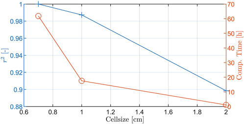
FIGURE 14. Convergence on cell size.

6.2 Settings of Reef3D

Settings made within the input file of Reef3D which are not on default and which are not specific to the computing server used (like the number of cores) or the output (like the time step of vtk. output files) are summarized in Table 6.

TABLE 6

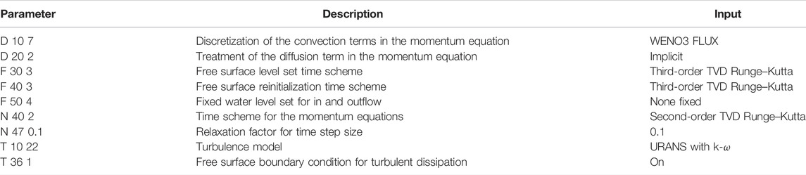
TABLE 6. Settings of Reef3D.