Topology and spectral interconnectivities of higher-order multilayer networks

1 Introduction

Multilayer networks (De Domenico et al., 2013; Boccaletti et al., 2014; Kivelä et al., 2014) have emerged over the last decade as a natural instrument in modeling myriads of heterogeneous systems. They permeate all areas of science as they provide a powerful abstraction of real-world phenomena made of interdependent sets of units interacting with each other through various channels. The concepts and computational methods they purvey have been the driving force for recent progress in the understanding of many highly sophisticated structures such as heterogeneous ecological systems (Pilosof et al., 2017; Timóteo et al., 2018), spatiotemporal and multimodal human brain connectomes (Griffa et al., 2017; Mandke et al., 2018; Pedersen et al., 2018), gene–molecule–metabolite interactions (Liu et al., 2020), and interdisciplinary scientific collaborations (Vasilyeva et al., 2021). This success has led to a growing interdisciplinary research investigating fundamental properties and topological invariants in multilayer networks.

Some of the major challenges in the analysis of a multilayer network are to quantify the importance and interdependence among its different components and subsystems, and describe the topological structures of the underlying architecture to better grasp the dynamics and information flow between its different network layers. Various approaches extending concepts, properties, and centrality indices from network science (Newman, 2003; Fortunato and Hric, 2016) have been developed, leading to tremendous results in many areas of science (Solá et al., 2013; Boccaletti et al., 2014; Sánchez-García et al., 2014; Flores and Romance, 2018; Timóteo et al., 2018; Wu et al., 2019; Liu et al., 2020; Yuvaraj et al., 2021). However, these approaches assume that inter- and intra-communications and relationships between the networks involved in such systems rely solely on node-based interactions. The resulting methods are, therefore, less insightful when the infrastructure is made up of higher-order intra- and inter-connectivities among node aggregations from different layers—as is the case for many phenomena. For example, heterogeneous ecosystems are made up of interactions among groups of the same or different species, social networks often connect groups of people belonging to different circles, and collaborations and citations form a higher-order multilayer network made of teams of co-authors interconnected to articles. Many recent studies have explored higher-order interactions and structures in monolayer networks (Benson et al., 2016; Iacopini et al., 2019; Lucas et al., 2020; Schaub et al., 2020; Bianconi, 2021) using different languages, such as simplicial complexes and hypergraphs (Shi et al., 2021; Young et al., 2021; Lotito et al., 2022; Majhi et al., 2022). However, a general mathematical formalism for modeling and studying higher-order multilayer networks is still lacking.

Our goal in this study is twofold. First, we propose a mathematical formalism that is rich enough to model and analyze multilayer complex systems involving higher-order connectivities within and in-between their subsystems. Second, we establish a unified framework for studying topological structures in such systems. This is performed by introducing the concepts of crossimplicial multicomplex, cross-homology, cross-Betti vectors, and cross-Laplacians. Before we dive deeper into these notions, we shall give the intuition behind them by considering the simple case of an undirected two-layered network Γ; here, Γ consists of two graphs (V₁, E₁) and (V₂, E₂), where V₁, V₂ are the node sets of Γ, E_s ⊆ V_s × V_s, s = 1, 2 are the sets of intra-layer edges, and a set E_1,2 ⊆ V₁ × V₂ of inter-layer edges. Intuitively, Γ might be seen as a system of interactions between two networks. It means that the node set V₁ interacts not only with V₂ but also with the edge set E₂ and vice versa. Similarly, intra-layer edges in one layer interact with edges and triads in the other layer, and so on. This view suggests a more combinatorial representation by some kind of two-dimensional generalization of the fundamental notion of simplicial complex from algebraic topology (Mac Lane, 1963; Hatcher, 2000). The idea of crossimplicial multicomplex defined in the present work allows such a representation. In particular, when applied to a pairwise-based multilayer network, this concept allows to incorporate, on one hand, the clique complexes (Lim, 2020; Schaub et al., 2020) corresponding to the network layers, and on the other, the clique complex representing the inter-layer relationships between the different layers into one single mathematical object. Moreover, Γ can be regarded through different lenses, and each view displays different kinds of topological structures. The most naive perspective flattens the whole structure into a monolayer network without segregating the nodes and links from one layer or the other. Another viewpoint is of two networks with independent or interdependent topologies communicating with each other through the inter-layer links. The rationale for defining cross-homology and the cross-Laplacians is to view Γ as different systems, each with its own intrinsic topology but in which nodes, links, etc., from one system have some restructuring power that allows them to impose and control additional topologies on the other. This means that in a multilayer system, a layer network might display different topological structures depending on whether we look at it from its own point of view, from the lens of the other layers, or as a part of a whole aggregated structure. We describe this phenomenon by focusing on the spectra and eigenvectors of the lower-degree cross-Laplacians. We shall, however, remark that our aim here is not to address a particular real-world problem but to provide broader mathematical settings that reveal and quantify the emergence of these structures in any type of multilayer network.

2 Crossimplicial multicomplexes

2.1 General definitions

Given two finite sets, V₁ and V₂, and a pair of integers k, l ≥−1, a (k, l)– crossimplex a in V₁ × V₂ is a subset $\{v_0^1,\dots ,v_k^1,v_0^2,\dots ,v_l^2\}$ of $V_1^{k+1}\times V_2^{l+1}$, where $v_i^s\in V_s$ for s = 1, 2. The point $v_i^1$ (resp. $v_j^2$) is the vertex of a in V₁ (resp. V₂), and its crossfaces are its subsets of the form $\{v_0^1,\dots ,v_{i-1}^1,v_{i+1}^1,\dots ,v_k^1,v_0^2,\dots ,v_l^2\}$ for 0 ≤ i ≤ k and $\{v_0^1,\dots ,v_k^1,v_0^2,\dots ,v_{i-1}^2,v_{i+1}^2,\dots ,v_l^2\}$ for 0 ≤ i ≤ l. Note that here we have used the conventions that $V_1^n\times V_2^0=V_1^n$ and $V_1^0\times V_2^n=V_2^n$.

An abstract crossimplicial bicomplex X (or a CSB) on V₁ and V₂ is a collection of crossimplices in V₁ × V₂, which is closed under the inclusion of crossfaces, i.e., the crossface of a crossimplex is also a crossimplex. A crossimplex is maximal if it is not the crossface of any other crossimplex. V₁ and V₂ are called the vertex sets of X.

Given a CSB X, for fixed integers k, l ≥ 0, we denote, by X_k,l, the subset of all its (k, l)-crossimplices. We also use the notations X_0,−1 = V₁, X_−1,0 = V₂, and X_−1,−1 =∅. Recursively, X_k,−1 will denote the subset of crossimplices of the form $\{v_0^1,\dots ,v_k^1\}\subset V_1^{k+1}$, and X_−1,l as the subset of crossimplices of the form $\{v_0^2,\dots ,v_l^2\}\subset V_2^{l+1}$. Such crossimplices will be referred to as intralayer simplices or horizontal simplices. We then obtain two simplicial complexes (Hatcher, 2000), X_•,−1 and X_−1,•, that we will refer to as the intralayer complexes and whose vertex sets are V₁ and V₂, respectively. In particular, X_1,−1 and X_−1,1 are graphs with vertex sets V₁ and V₂, respectively.

The dimension of a (k, l)-crossimplex is k + l + 1, and the dimension of CSB X is the dimension of its crossimplices of the highest dimension. The n-skeleton of X is the restriction of X to (k, l)-crossimplices such that k + l + 1 ≤ n. In particular, the 1-skeleton of CSB is a two-layered network, with X_0,0 being the set of inter-layer links. Conversely, given a two-layered network Γ formed by two graphs Γ₁ = (V₁, E₁) and Γ₂ = (E₂, V₂) with the inter-layer edge set E_1,2 ⊂ V₁ × V₂, define a (k, l)-clique in Γ as a pair (σ₁, σ₂), where σ₁ is a k-clique in Γ₁ and σ₂ is an l-clique in Γ₂ with the property that (i, j) ∈ E_1,2 for every i ∈ σ₁ and j ∈ σ₂. We define the cross-clique bicomplex X associated with Γ by letting X_k,l to be the set of all (k + 1, l + 1)-cliques in Γ.

Now, a crossimplicial multicomplex (CSM) $\mathcal{X}$ consists of a family of finite sets $V_s,s\in S\subseteq \mathbb{N}$ and a CSB ${\mathcal{X}}^{s,t}$ for each pair of distinct indices s, t ∈ S. It is undirected if the sets of crossimplices in ${\mathcal{X}}^{s,t}$ and ${\mathcal{X}}^{t,s}$ are in one-to-one correspondence. In such a case, $\mathcal{X}$ is completely defined by the family of CSB ${\mathcal{X}}^{s,t}$ with s < t (see Figure 2 for a visualization of a three-layered CSM).

2.2 Orientation on crossimplices

The orientation of a (k, l)-crossimplex is an ordering choice over its vertices. When equipped with an orientation, the crossimplex is said to be oriented and will be represented as $[a]=[v_0^1,\dots ,v_k^1;v_0^2,\dots ,v_l^2]$ if k, l ≥ 0, or $[v_0^1,\dots ,v_k^1]$ (resp. $[v_0^2,\dots ,v_l^2]$) if k ≥ 0 and l = −1 (resp. k = −1 and l ≤ 0). We shall note that an orientation of crossimplices is just a choice purely made for computational purposes. Extending geometric representations from simplicial complexes, crossimplices can be represented as geometric objects.

Specifically, a (0, −1)-crossimplex is a vertex in the top layer; a (0,0)-crossimplex is a cross-edge between layers V₁ and V₂; a (1, −1)-crossimplex (resp (−1, 1)-crossimplex) is a horizontal edge on V₁ (resp. V₂); a (0,1)-crossimplex or a (1,0)-crossimplex is a cross-triangle; a (2, −1)-crossimplex or (−1, 2)-crossimplex is a horizontal triangle on layer V₁ or V₂; a (3, −1)-crossimplex or (−1, 3)-crossimplex is a horizontal tetrahedron on V₁ or V₂; and a (1,1)-crossimplex, a (2,0)-crossimplex, or a (0,2)-crossimplex is a cross-tetrahedron (see Figure 1 for illustrations). On the other hand, horizontal edges, triangles, tetrahedrons, are just usual simplices on the horizontal complexes. One can consider a cross-edge as a connection between a vertex from one layer to a vertex on the other layer. In the same vein, a cross-triangle can be considered a connection between a vertex from one layer and two vertices on the other, and a cross-tetrahedron as a connection between either two vertices from one layer and two vertices on the other, or one vertex from one layer to three vertices on the other.

FIGURE 1

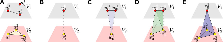
FIGURE 1. Crossimplices. Schematic representation of (A) A (0, −1)-crossimplex (a top vertex), a (1, −1)-crossimplex (top horizontal edge), and a (−1, 2)-crossimplex (bottom horizontal triangle); (B) (0,0)-crossimplex (a cross-edge); (C) (1,0)-crossimplex (a top cross-triangle); (D) (1,1)-crossimplex (a cross-tetrahedron); and (E) (0,2)-crossimplex (also a cross-tetrahedron). Notice that cross-edges are always oriented from the vertex of the top layer to that in the bottom layer. Therefore, cross-edges belonging to a cross-triangle are always of opposite orientations with respect to any orientation of the cross-triangle. There are two types of cross-triangles: the (1,0)-crossimplices (top cross-triangles) and (0,1)-crossimplices (bottom cross-triangle). Moreover, there are three types of cross-tetrahedrons: the (0,2)-crossimplices, (2,0)-crossimplices, and (1,1)-crossimplices.

2.3 Weighted CSBs

A weight on CSB X is a positive function $w:{\bigcup }_{k,l}{X}_{k,l}\to {\mathbb{R}}^{+}$ that does not depend on the orientations of crossimplices. A weighted CSB is one that is endowed with a weight function. The weight of a crossimplex a ∈ X is the number w(a).

3 Topological descriptors

3.1 Cross-boundaries

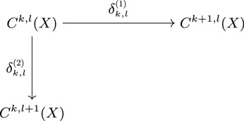
CSB X defines a bi-simplicial set (Moerdijk, 1989; Goerss and Jardine, 2009) by considering, respectively, the top and bottom crossface maps $d_{i|k,l}^{(1)}:X_{k,l}\to X_{k-1,l}$ and $d_{i|k,l}^{(2)}:X_{k,l}\to X_{k,l-1}$ by

$\begin{array}{cc}\hfill d_{i|k,l}^{(1)}\left([v_0^1,\dots ,v_k^1;v_0^2,\dots ,v_l^2]\right)& =\left[v_0^1,\dots ,\widehat{v_i^1},\dots ,v_k^1;v_0^2,\dots ,v_l^2\right]\hfill \\ \hfill d_{i|k,l}^{(2)}\left([v_0^1,\dots ,v_k^1;v_0^2,\dots ,v_l^2]\right)& =\left[v_0^1,\dots ,v_k^1;v_0^2,\dots ,\widehat{v_i^2},\dots ,v_k^2\right],\hfill \end{array}(1)$

where the hat over a vertex means dropping the vertex. Moreover, for a fixed l ≥−1, $X_{•,l}={(X_{k,l})}_{k\ge -1}$ is a simplicial complex. Similarly, $X_{k,•}={(X_{k,l})}_{l\ge -1}$ is a simplicial complex. We observe that if $a=\{v_0^1,\dots ,v_k^1,v_0^2,\dots ,v_l^2\}\in X_{k,l}$, then $a^{(1)}=\{v_0^1,\dots ,v_k^1\}\in X_{k,-1}$ and $a^{(2)}=\{v_0^2,\dots ,v_l^2\}\in X_{-1,l}$. We will refer to a⁽¹⁾ and a⁽²⁾ as the top horizontal face and the bottom horizontal face of a, respectively. Conversely, two horizontal simplices, v¹ ∈ X_k,−1 and v² ∈ X_−1,l, are said to be interconnected in X if they are, respectively, the top and bottom horizontal faces of a (k, l)-crossimplex a. We then write v¹ ∼ v². This is equivalent to requiring that if $v^1=\{v_0^1,\dots ,v_k^1\}$ and $v^2=\{v_0^2,\dots ,v_l^2\}$, then $\{v_0^1,\dots ,v_k^1,v_0^2,\dots ,v_l^2\}\in X_{k,l}$. If $a=\{v_0^1,\dots ,v_k^1,v_0^2,\dots ,v_l^2\}\in X_{k,l}$, we define its top cross-boundary ${\partial }_{}^{(1)}a$ as the subset of X_k−1,l consisting of all the top crossfaces of a, i.e., all the (k − 1, l)-crossimplices of the form $d_{i|k,l}^{(1)}[a]$ for i = 0, … , k. Analogously, its bottom cross-boundary ${\partial }_{}^{(2)}a\subseteq X_{k,l-1}$ is the subset of all its bottom crossfaces $d_{i|k,l}^{(2)}[a],i=0,\dots ,l$.

Now, two (k, l)-crossimplices a, b ∈ X_k,l are said to be as follows:

• top-outer (TO) adjacent, which we write $a{⌢}_{}^{(1)}b$ or $a{⌢}_c^{(1)}b$, if both are top crossfaces of a (k + 1, l)-crossimplex c; in other words, $a,b\in {\partial }_{}^{(1)}c$;

• top-inner (TI) adjacent, which we write $a{⌣}_{(1)}^{}b$ or $a{⌣}_{(1)}^{d}b$, if there exists a (k − 1, l)-crossimplex d ∈ X_k−1,l, which is a top crossface of both a and b, i.e., $d\in {\partial }_{}^{(1)}a\cap {\partial }_b^{(1)}$;

• bottom-outer (BO) adjacent, which we write $a{⌢}_b^{(2)}$ or $a{⌢}_c^{(2)}b$, if both are bottom crossfaces of a (k, l + 1)-crossimplex c ∈ X_k,l+1; in other words, $a,b\in {\partial }_{}^{(2)}c$; and

• bottom-inner (BI) adjacent, which we write $a{⌣}_{(2)}^{}b$ or $a{⌣}_{(2)}^{d}b$, if there exists a (k, l − 1)-crossimplex f ∈ X_k,l−1, which is a bottom face of both a and b; i.e., $d\in {\partial }_{}^{(2)}a\cap {\partial }_{}^{(2)}b$.

3.2 Degrees of crossimplices

Given a weight function w on X, we define the following degrees of a (k, l)-crossimplex a relative to w.

• The TO degree of a is the number:

${\mathrm{deg}}_{TO}\left(a\right)={\mathrm{deg}}_{TO}\left(a,w\right)≔{\displaystyle \sum _{\stackrel{a^{\prime }\in X_{k+1,l}}{a\in {\partial }_{}^{(1)}{a}^{\prime }}}}w\left(a^{\prime }\right).(2)$

• Similarly, the TI degree of a is defined as follows:

${\mathrm{deg}}_{TI}\left(a\right)={\mathrm{deg}}_{TI}\left(a,w\right)≔{\displaystyle \sum _{\stackrel{c\in X_{k-1,l}}{c\in {\partial }_{}^{(1)}a}}}\frac{1}{w\left(c\right)}.(3)$

• Analogously, the BO degree of a is given as follows:

${\mathrm{deg}}_{BO}\left(a\right)={\mathrm{deg}}_{BO}\left(a,w\right)≔{\displaystyle \sum _{\stackrel{a^{\prime }\in X_{k,l+1}}{a\in {\partial }_{}^{(2)}{a}^{\prime }}}}w\left(a^{\prime }\right).(4)$

• The BO degree of a is as follows:

${\mathrm{deg}}_{BI}\left(a\right)={\mathrm{deg}}_{BI}\left(a,w\right)≔\sum _{\stackrel{c\in X_{k,l-1}}{c\in {\partial }_{}^{(2)}a}}\frac{1}{w\left(c\right)}.(5)$

Observe that in the particular case where the weight function is equal to one everywhere, the TO degree of a is precisely the number of (k + 1, l)-crossimplices in X, of which a is the top crossface, while deg_TI(a) is the number of top crossfaces of a, which equals to k + 1. Analogous observations can be made about the BO and BI degrees.

3.3 Cross-homology groups

The space C_k,l of (k, l)-cross-chains is defined as the real vector space generated by all oriented (k, l)-crossimplexes in $\mathcal{X}$. The top and bottom cross-boundary operators ${\partial }_{k,l}^{(1)}:C_{k,l}\to C_{k-1,l}$ and ${\partial }_{k,l}^{(2)}:C_{k,l}\to C_{k,l-1}$ are then defined as follows by the formula

${\partial }_{k,l}^{(s)}\left(\left[a\right]\right)≔{\displaystyle \sum _{b\in {\partial }_{}^{(s)}a}}\mathrm{s}\mathrm{g}\mathrm{n}\left(b,{\partial }_{}^{(s)}a\right)\left[b\right],(6)$

for s = 1, 2 and a generator a ∈ X_k,l, where $\mathrm{s}\mathrm{g}\mathrm{n}(b,{\partial }_{}^{(s)}a)$ is the sign of the orientation of b in ${\partial }_{}^{(s)}a$; in other words, if $b=d_{i|k,l}^{(1)}[a]$, then $\mathrm{s}\mathrm{g}\mathrm{n}(b,{\partial }_{}^{(1)}a)≔{(-1)}^i$, and we define $\mathrm{s}\mathrm{g}\mathrm{n}(b,{\partial }_{}^{(2)}a)$ in a similar fashion.

It is straightforward to see that in particular

${\partial }_{k,-1}^{(1)}:C_{k,-1}\to C_{k-1,-1},k\ge 0$

and

${\partial }_{-1,l}^{(2)}:C_{-1,l}\to C_{-1,l},l\ge 0$

are the usual boundary maps of simplicial complexes. For this reason, we focus more on the mixed case where both l and k are non-negative. We will often drop the indices and write ∂⁽¹⁾ and ∂⁽²⁾ to avoid cumbersome notations. To see how these maps operate, let us compute, for instance, the images of the crossimplices (b), (c), (d), and (e) illustrated in Figure 1. We obtain the following:

$\left\{\begin{array}{c}{\partial }_{\mathrm{0,0}}^{(1)}\left[v_0^1;v_0^2\right]=\left[v_0^2\right]\in C_{-\mathrm{1,0}}\hfill \\ \hfill \\ {\partial }_{\mathrm{0,0}}^{(2)}\left[v_0^1;v_0^2\right]=-\left[v_0^1\right]\in C_{0,-1};\hfill \end{array}\right.$

$\left\{\begin{array}{c}{\partial }_{\mathrm{1,0}}^{(1)}\left[w_0^1,w_1^1;w_0^2\right]=\left[w_1^1;w_0^2\right]-\left[w_0^1;w_0^2\right]\in C_{\mathrm{0,0}},\hfill \\ \hfill \\ {\partial }_{\mathrm{1,0}}^{(2)}\left[w_0^1,w_1^1;w_0^2\right]=\left[w_0^1,w_1^1\right]\in C_{1,-1};\hfill \end{array}\right.$

$\left\{\begin{array}{c}{\partial }_{\mathrm{1,1}}^{(1)}\left[w_0^1,w_1^1;w_0^2,w_1^2\right]=\left[w_1^1;w_0^2,w_1^2\right]-\left[w_0^1;w_0^2,w_0^2\right]\in C_{\mathrm{0,1}},\hfill \\ \hfill \\ {\partial }_{\mathrm{1,1}}^{(2)}\left[w_0^1,w_1^1;w_0^2,w_1^2\right]=\left[w_0^1,w_1^1;w_1^2\right]-\left[w_0^1,w_1^1;w_0^2\right]\in C_{\mathrm{1,0}};\hfill \end{array}\right.$

$\left\{\begin{array}{c}{\partial }_{\mathrm{0,2}}^{(1)}\left[z_0^1;z_0^2,z_1^2,z_2^2\right]=\left[z_0^2,z_1^2,z_2^2\right]\in C_{-\mathrm{1,2}}\hfill \\ \hfill \\ {\partial }_{\mathrm{0,2}}^{(2)}\left[z_0^1;z_0^2,z_1^2,z_2^2\right]=\left[z_0^1;z_1^2,z_2^2\right]-\left[z_0^1;z_0^2,z_2^2\right]\hfill \\ +\left[z_0^1;z_0^2,z_1^2\right]\in C_{\mathrm{0,1}}.\hfill \end{array}\right.$

Notice that ${\partial }_{0,-1}^{(1)}={\partial }_{-\mathrm{1,0}}^{(2)}=0$. Moreover, by simple calculations from (6), it is easy to check that ${\partial }_{k-1,l}^{(1)}{\partial }_{k,l}^{(1)}=0$ and ${\partial }_{k,l-1}^{(2)}{\partial }_{k,l}^{(2)}=0$, which allows to define the top and bottom (k, l)-cross-homology groups of X as the following quotients:

${\text{H}}_{k,l}^{(1)}\left(X\right)≔\ker {\partial }_{k,l}^{(1)}/\mathrm{i}\mathrm{m}{\partial }_{k+1,l}^{(1)},\mathrm{a}\mathrm{n}\mathrm{d}$

${\text{H}}_{k,l}^{(2)}\left(X\right)≔\ker {\partial }_{k,l}^{(2)}/\mathrm{i}\mathrm{m}{\partial }_{k,l+1}^{(2)}.$

For k ≥ 0 and l ≤ 0, ${\partial }_{k,-1}^{(1)}$ and ${\partial }_{-1,l}^{(2)}$ are the usual boundary maps of simplicial complexes (Hatcher, 2000). Therefore, ${\text{H}}_{k,-1}^{(1)}(X)$ and ${\text{H}}_{-1,l}^{(2)}(X)$ are the usual homology groups (Mac Lane, 1963; Hatcher, 2000) of the simplicial complexes X_•,−1 and X_−1,•, respectively.

3.4 Cross-Betti vectors

The cross-homology groups are completely determined by their dimensions, the top and bottom (k, l)-cross-Betti numbers ${\beta }_{k,l}^{(s)}(X)=\dim {\text{H}}_{k,l}^{(s)}(X)$, s = 1, 2. In particular, ${\beta }_{k,-1}^{(1)}$ and ${\beta }_{-1,l}^{(2)}$ are the usual Betti numbers for the horizontal simplicial complexes (Hatcher, 2000). The couple ${\beta }_{k,l}=({\beta }_{k,l}^{(1)},{\beta }_{k,l}^{(2)})$ is the (k, l)-cross-Betti vector of X and can be computed using basic linear algebra. These vectors are descriptors of the topologies of both the horizontal complexes and their inter-connections. For instance, β_0,−1 and β_−1,0 encode the connectivities within and in-between the 1-skeletons of the horizontal complexes associated with X. Precisely, ${\beta }_{0,-1}^{(1)}$ is the number of connected components of the graph X_1,−1, and ${\beta }_{0,-1}^{(2)}$ is the number of nodes in V₁ with no interconnections with any nodes in V₂. Similarly, ${\beta }_{-\mathrm{1,0}}^{(1)}$ is the number of nodes in V₂ with no interconnections with any nodes in V₁, while ${\beta }_{-\mathrm{1,0}}^{(2)}$ is the number of connected components of the bottom horizontal graph X_−1,1. Furthermore, β_1,−1 simultaneously counts the number of loops in X_1,−1 and the number of its intra-layer links that do not belong to cross-triangles formed with the graph X_−1,1. Analogous topological information is provided by β_−1,1. In addition, β_0,0 measures the extent to which individual nodes of one complex layer serve as communication channels between different hubs from the other layers. More precisely, an element in ${\text{H}}_{\mathrm{0,0}}^{(1)}(X)$ represents either an inter-layer one-dimensional loop formed by a path in X_1,−1, whose end-nodes interconnect with the same node in V₂, or two connected components in the top complex communicating with each other through a node in the bottom complex. β_0,0 counts the shortest paths of length 2 between nodes within one layer passing through a node from the other layer and not belonging to the cross-boundaries of cross-triangles; we call such paths cones. In other words, β_0,0 quantifies node clusters in one layer that are “controlled” by nodes in the other layer. Detailed proof of this description is provided in Methods 7.1.

Now, given a CSM $\mathcal{X}$, its cross-Betti table ${\beta }_{k,l}^{\otimes }$ is obtained by computing all the cross-Betti vectors of all its underlying CSBs. Computation of the cross-Betti table of the CSM of Figure 2 is presented in Table 1.

FIGURE 2

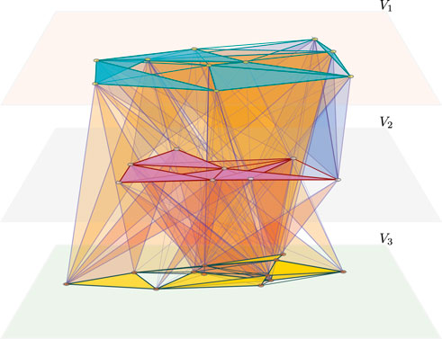
FIGURE 2. Schematic representation of a two-dimensional crossimplicial multicomplex $\mathcal{X}$ with 3 layers and 30 nodes in total; $\mathcal{X}$ consists of the vertex sets V₁, V₂, and V₃ and the three CSBs ${\mathcal{X}}^{\mathrm{1,2}},{\mathcal{X}}^{\mathrm{1,3}},{\mathcal{X}}^{\mathrm{2,3}}$ defined, respectively, on the products V₁ × V₂, V₁ × V₃, and V₂ × V₃.

TABLE 1

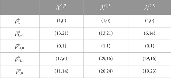
TABLE 1. Cross-Betti table. The cross-Betti table for CSM of Figure 2. The table quantifies the connectedness of the three horizontal complexes, the number of cycles in each of them, the number of nodes in each layer that are not connected to the other layers, the number of intra-layer edges not belonging to any cross-triangles, and the number of paths of length 2 connecting the nodes in one layer and passing through a node from another layer.

To illustrate what the cross-Betti vectors represent, we consider the simple two-dimensional CSB X of Figure 3. We get ${\beta }_{0,-1}^{(1)}=2,{\beta }_{1,-1}^{(1)}=1$ and ${\beta }_{-\mathrm{1,0}}^{(2)}=1,{\beta }_{-\mathrm{1,1}}^{(2)}=0$. This reflects the fact the top layer has two connected components and one cycle, while the bottom one has one component and no cycles. Moreover, three top nodes are not interconnected to the bottom complex, six top edges are not top faces of cross-triangles, two bottom nodes are not interconnected to the top layer, and five bottom edges are not bottom faces of cross-triangles. This information is encoded in β_0,−1 = (2, 3), β_1,−1 = (1, 6), β_−1,0 = (2, 1), and β_−1,1 = (5, 0). There are three generating inter-layer cycles, two of which are formed by an intra-layer path in the bottom layer and a node in the top layer ($v_4^1$ and $v_6^1$), and the other one is formed by an intra-layer path in the top layer and a node $(v_1^2)$ in the bottom layer. Moreover, the two nodes $v_1^2$ and $v_4^2$ of V₂ interconnect the two separated components of the top layer; they serve as cross-hubs: removing both nodes eliminates all communications between the two components of the top layer. Cross-hubs and these types of inter-layer cycles are exactly what β_0,0 encodes. Specifically, by computing the cross-homology of X, we get ${\beta }_{\mathrm{0,0}}^{(1)}=3$, which counts the cycle $v_2^1-v_3^1-v_4^1-v_1^2-v_2^1$ and the nodes $v_4^2$ and $v_1^2$ that interconnect $v_4^1$ to $v_6^1$, and $v_2^1$ to $v_6^1$, ${\beta }_{\mathrm{0,0}}^{(2)}=2$ counting the inter-layer cycles $v_4^1-v_1^2-v_2^2-v_3^2-v_4^2-v_4^1$ and $v_6^1-v_2^2-v_3^2-v_4^2-v_6^1$. In each of these cycles, the top node allows a shortest (inter-layer) path between the end-points of the involved intra-layer path.

FIGURE 3

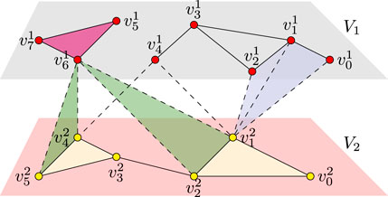
FIGURE 3. Cross-Betti vectors. Schematic representation of a two-dimensional CSB with 14 nodes in total, whose oriented maximal crossimplices are the intra-layer triangle $[v_5^1,v_6^1,v_7^1]$ in X_2,−1, the intra-layer edges $[v_0^1,v_1^1],[v_1^1,v_2^1],[v_1^1,v_3^1],[v_2^1,v_3^1]$ in X_1,−1, the bottom intra-layer triangles $[v_0^2,v_1^2,v_2^2],[v_3^2,v_4^2,v_5^2]$ in X_−1,2, the intra-layer edge $[v_2^2,v_3^2]$ in X_−1,1, the cross-triangles $[v_0^1,v_1^1;v_1^2],[v_1^1,v_2^1;v_1^2]$ in X_1,0, $[v_6^1;v_1^2,v_2^2],[v_6^1;v_4^2,v_5^2]$ in X_0,1, and the cross-edges $[v_4^1;v_1^2],[v_4^1;v_4^2]$ in X_0,0.

Using algebraic topological methods to calculate the cross-Betti vectors for larger multicomplexes can quickly become computationally heavy. We provide powerful linear-algebraic tools that not only allow to easily compute β_k,ls but also tell exactly where the topological structures being counted are located within the multicomplex.

4 Spectral descriptors

4.1 Cross-forms

$C^{k,l}≔C^{k,l}(X,\mathbb{R})$ denotes the dual space ${\mathrm{H}\mathrm{o}\mathrm{m}}_{\mathbb{R}}(C_{k,l},\mathbb{R})$ of the real vector space C_k,l. In other words, C^k,l is the vector space of real linear functional $\varphi :C_{k,l}\to \mathbb{R}$. We will refer to such functionals as (k, l)-forms or cross-forms on X. In particular, (k, −1)-forms correspond to k-forms on the simplicial complex X_•,−1, and (−1, l)-forms are l-forms on the complex X_−1,•. We have C^−1,−1 = 0, and by convention, we set C^k,l (∅) = 0.

Notice that a natural basis of C^k,l is given by the following set of linear forms:

$\left\{e_a:C_{k,l}\to \mathbb{R},a\in X_{k,l}\right\},$

called elementary cross-forms, where

$e_a\left(b\right)=\left\{\begin{array}{cc}1,\hfill & \text{if\hspace{0.17em}\hspace{0.17em}}a=b,\hfill \\ 0,\hfill & \mathrm{o}\mathrm{t}\mathrm{h}\mathrm{e}\mathrm{r}\mathrm{w}\mathrm{i}\mathrm{s}\mathrm{e},\hfill \end{array}\right.$

which naturally identify C^k,l with C_k,l. Now, the maps ${\delta }_{k,l}^{(1)}:C^{k,l}\to C^{k+1,l}$ and ${\delta }_{k,l}^{(2)}:C^{k,l}\to C^{k,l+1}$ are defined by the following equations:

$\begin{array}{cc}\hfill {\delta }_{k,l}^{(1)}\varphi \left(\left[a\right]\right)& ={\displaystyle \sum _{b\in {\partial }_{}^{(1)}a}}\mathrm{s}\mathrm{g}\mathrm{n}\left(b,{\partial }_{}^{(1)}a\right)\varphi \left(\left[b\right]\right),\hfill \\ \hfill {\delta }_{k,l}^{(2)}\varphi \left(\left[c\right]\right)& ={\displaystyle \sum _{d\in {\partial }_{}^{(2)}c}}\mathrm{s}\mathrm{g}\mathrm{n}\left(d,{\partial }_{}^{(2)}c\right)\varphi \left(\left[d\right]\right),\hfill \end{array}(7)$

for ϕ ∈ C^k,l, a ∈ X_k+1,l and c ∈ X_k,l+1. Next, given a weight w on X, we get an inner product on cross-forms by the following setting:

${⟨\varphi ,\psi ⟩}_{k,l}≔{\displaystyle \sum _{a\in X_{k,l}}}w\left(a\right)\varphi \left(a\right)\psi \left(a\right),\text{for\hspace{0.17em}\hspace{0.17em}}\varphi ,\psi \in C^{k,l}.(8)$

It can been seen that, with respect to this inner product, elementary cross-forms form an orthogonal basis, and by simple calculations, the dual maps are given by the following equation:

${\left({\delta }_{k,l}^{(1)}\right)}^{*}\varphi \left(\left[a\right]\right)={\displaystyle \sum _{\stackrel{a^{\prime }\in X_{k+1,l}}{a\in {\partial }_{}^{(1)}{a}^{\prime }}}}\frac{w\left(a^{\prime }\right)}{w\left(a\right)}\mathrm{s}\mathrm{g}\mathrm{n}\left(a,{\partial }_{}^{(1)}{a}^{\prime }\right)\varphi \left(\left[a^{\prime }\right]\right),(9)$

for ϕ ∈ C^k+1,l, a ∈ X_k,l. We also obtain a similar formula for the dual ${({\delta }_{k,l}^{(2)})}^{*}$.

4.2 The cross-Laplacian operators

Identifying C_k,l with C^k,l and equipping it with an inner product, as (21), we define the following self-adjoint linear operators on C_k,l for all k, l ≥−1:

- the top (k, l)-cross-Laplacian is as follows:

${\mathcal{L}}_{k,l}^{(\mathrm{T})}≔{\left({\delta }_{k,l}^{(1)}\right)}^{*}{\delta }_{k,l}^{(1)}+{\delta }_{k-1,l}^{(1)}{\left({\delta }_{k-1,l}^{(1)}\right)}^{*};$

- and the bottom (k, l)-cross-Laplacian is as follows:

${\mathcal{L}}_{k,l}^{(\mathrm{B})}≔{\left({\delta }_{k,l}^{(2)}\right)}^{*}{\delta }_{k,l}^{(2)}+{\delta }_{k,l-1}^{(2)}{\left({\delta }_{k,l-1}^{(2)}\right)}^{*}.$

Being defined on finite dimensional spaces, these operators can be represented as square matrices indexed over crossimplices. Specifically, denoting N_k,l = |X_k,l|, ${\mathcal{L}}_{k,l}^{(\mathrm{T})}$ can be represented by positive definite N_k,l × N_k,l matrices (see Methods 7.3).

Moreover, the null spaces, the elements of which we call harmonic cross-forms, are easily seen to be in one-to-one correspondence with cross-cycles on X. In other words, we have the following isomorphisms (see Methods 7.2 for the proof):

${\text{H}}_{k,l}^{(1)}\left(X\right)\cong \ker {\mathcal{L}}_{k,l}^{(\mathrm{T})},{\text{H}}_{k,l}^{(2)}\left(X\right)\cong \ker {\mathcal{L}}_{k,l}^{(\mathrm{B})}.$

It follows that in order to compute the cross-Betti vectors, it suffices to determine the dimensions of the eigenspaces of the zero-eigenvalues of the cross-Laplacians.

It should be noted that in addition to being much easier to implement, the spectral method to compute cross-homology has the advantage of providing a geometric representation of the cross-Betti numbers through eigenvectors. However, before we see how this works, let us make a few observations. Notice that ${\mathcal{L}}_{0,-1}^{(\mathrm{T})}$ and ${\mathcal{L}}_{-\mathrm{1,0}}^{(\mathrm{B})}$ are the usual graph Laplacians of 0 degree for the horizontal complexes. More generally, ${\mathcal{L}}_{k,-1}^{(\mathrm{T})}$ and ${\mathcal{L}}_{-1,l}^{(\mathrm{B})}$ are the combinatorial higher Hodge Laplacians (Horak and Jost, 2013; Lim, 2020; Schaub et al., 2020) of degrees k and l, respectively, for the horizontal simplicial complexes. Furthermore, ${\mathcal{L}}_{k,-1}^{(\mathrm{B})}$ (resp. ${\mathcal{L}}_{-1,l}^{(\mathrm{T})}$) detects the k-simplices (resp. l-simplices) in the top (resp. bottom) layer complex that are not top (resp. bottom) faces of (k, 0)-crossimplices (resp. (0, l)-crossimplices). Moreover, one can see that ${\mathcal{L}}_{k,-1}^{(\mathrm{B})}$ is the diagonal matrix indexed over the k-simplices on the top complex and whose diagonal entries are the BO degrees. Similarly, ${\mathcal{L}}_{-1,l}^{(\mathrm{T})}$ is the diagonal matrix whose diagonal entries are the TO degrees of the l-simplices on the bottom complex. This is consistent with the interpretation of the cross-Betti numbers ${\beta }_{0,-1}^{(2)}$ and ${\beta }_{-\mathrm{1,0}}^{(1)}$ given earlier in terms of connectivities between the 1-skeletons of the horizontal complexes.

4.3 Harmonic cross-hubs

For the sake of simplicity, it is assumed that X is equipped with the trivial weight ≅1. Then, by (26), the (0,0) cross-Laplacians ${\mathcal{L}}_{\mathrm{0,0}}^{(\mathrm{T})}$ and ${\mathcal{L}}_{\mathrm{0,0}}^{(\mathrm{B})}$ are, respectively, represented by the N_0,0 × N_0,0 matrices indexed on cross-edges a_i, a_j ∈ X_0,0, whose entries are given by the following equations:

${\left({\mathcal{L}}_{\mathrm{0,0}}^{(\mathrm{T})}\right)}_{a_i,a_j}=\left\{\begin{array}{c}{\mathrm{deg}}_{TO}\left(a_i\right)+1,\text{if\hspace{0.17em}}i=j,\hfill \\ \begin{array}{cc}1,\hfill & \text{if\hspace{0.17em}}i\ne j,\left[a_i\right]=\left[v_i^1;v_k^2\right],\hfill \\ \hfill & \left[a_j\right]=\left[v_j^1;v_k^2\right]\hfill \\ \hfill & \text{and\hspace{0.17em}}\left\{v_i^1,v_j^1,v_k^2\right\}\notin X_{\mathrm{1,0}},\hfill \end{array}\hfill \\ 0,\mathrm{o}\mathrm{t}\mathrm{h}\mathrm{e}\mathrm{r}\mathrm{w}\mathrm{i}\mathrm{s}\mathrm{e},\hfill \end{array}\right.(10)$

and

${\left({\mathcal{L}}_{\mathrm{0,0}}^{(\mathrm{B})}\right)}_{a_i,a_j}=\left\{\begin{array}{c}{\mathrm{deg}}_{BO}\left(a_i\right)+1,\text{if\hspace{0.17em}}i=j,\hfill \\ \begin{array}{cc}1,\hfill & \text{if\hspace{0.17em}}\left[a_i\right]=\left[v_{i_0}^1;v_i^2\right],\hfill \\ \hfill & \left[a_j\right]=\left[v_{i_0}^1;v_j^2\right],\hfill \\ \hfill & \text{and\hspace{0.17em}}\left\{v_{i_0}^1,v_i^2,v_j^2\right\}\notin X_{\mathrm{0,1}},\hfill \end{array}\hfill \\ 0,\mathrm{o}\mathrm{t}\mathrm{h}\mathrm{e}\mathrm{r}\mathrm{w}\mathrm{i}\mathrm{s}\mathrm{e}.\hfill \end{array}\right.(11)$

Applied to the toy example of Figure 3, ${\mathcal{L}}_{\mathrm{0,0}}^{(\mathrm{T})}$ has a zero-eigenvalue of multiplicity 3, generating the three (0,0) cross-cycles in Table 2.

TABLE 2

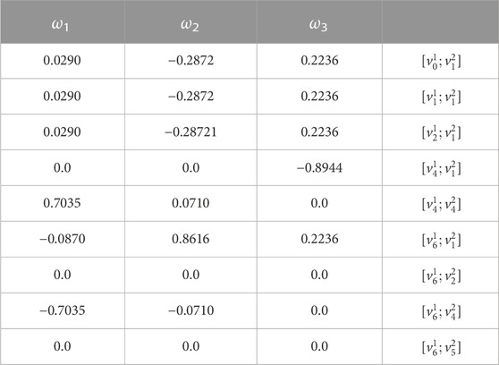
TABLE 2. Harmonic (0,0) cross-forms. The three eigenvectors of the eigenvalue 0 of ${\mathcal{L}}_{\mathrm{0,0}}^{(\mathrm{T})}$ corresponding to the synthetic CSB of Figure 3. There are two harmonic cross-hubs, $v_1^2$ and $v_4^2$, and their respective harmonic cross-hubness are 2.6177 and 1.4070.

Each coordinate in the eigenvectors is seen as an “intensity” along the corresponding cross-edge. Cross-edges with non-zero intensities sharing the same bottom node define certain communities in the top complex that are “controlled” by the involved bottom node. These community structures depend on both the underlying topology of the top complex and its interdependence with the other complex layer. We then refer to them as harmonic cross-clusters, and the bottom nodes controlling them are considered harmonic cross-hubs (HCHs). The harmonic cross-hubness of a bottom node is the L¹-norm of the intensities of all cross-edges having it in common. Here, in the eigenvectors of the eigenvalue 0, there are two subsets of cross-edges with non-zero coordinates: the cross-edges with $v_1^2$ in common and those with $v_4^2$ in common. We, therefore, have two harmonic cross-hubs (see illustration in Figure 4), hence two harmonic cross-clusters. The first harmonic cross-hub is responsible for the top layer cross-cluster $\{v_0^1,v_1^1,v_2^1,v_4^1,v_6^1\}$, while the second harmonic cross-hub controls the top layer cross-cluster $\{v_4^1,v_6^1\}$. The intensity of each involved cross-edge is the L¹-norm of its corresponding coordinates in the three eigenvectors, and the harmonic cross-hubness is the sum of the intensities of the cross-edges interconnecting the corresponding cross-hub to each of the top nodes in the cross-clusters it controls. For instance, $v_1^2$ is the bottom node with the highest harmonic cross-hubness, which is 2.6177. This reflects the fact that $v_1^2$ not only interconnects the two connected components of the top complex (which $v_4^2$ does as well) but it also allows fast-track connections between the highest number of nodes that are not directly connected with intra-layer edges in the top complex. The same calculations applied to the eigenvectors of the zero-eigenvalues of ${\mathcal{L}}_{\mathrm{0,0}}^{(\mathrm{B})}$ yield $v_6^1$ as the top node with the highest harmonic cross-hubness with respect to the bottom complex.

FIGURE 4

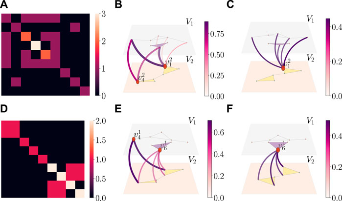
FIGURE 4. Cross-Laplacians, harmonic, and principal cross-hubs. (A) and (D) Heat-maps of the top and bottom (0,0) cross-Laplacian matrices for the example in Figure 3. Both matrices are indexed over the cross-edges of CSB, and the diagonal entries correspond to one added to the number of cross-triangles containing the corresponding cross-edge. ${\mathcal{L}}_{\mathrm{0,0}}^{(\mathrm{T})}$ has a zero eigenvalue of multiplicity 3, while ${\mathcal{L}}_{\mathrm{0,0}}^{(\mathrm{B})}$ has a zero eigenvalue of multiplicity 2. (B) and (E) Harmonic cross-hubs with respect to the top (resp. the bottom) horizontal complex of X; the intensity of a cross-edge is given by the L¹-norm of the corresponding coordinates in the eigenvectors of the eigenvalue 0. (C) and (F) Principal cross-hubs in the bottom (resp. top) layer with respect to the top (resp. bottom) layer; by definition, they are the spectral cross-hubs obtained from the largest eigenvalues of the top and bottom (0,0) cross-Laplacians, respectively.

4.4 Spectral persistence of cross-hubs

To better grasp the idea of cross-hubness, let us have a closer look at the coordinates of the eigenvectors of the (0,0) cross-Laplacians ((10) and (11)) whose eigenvalues are all non-negative real numbers. Suppose $\varphi =(x_1,\dots ,x_{N_{\mathrm{0,0}}})$ is an eigenvector for an eigenvalue λ^T of ${\mathcal{L}}_{\mathrm{0,0}}^{(\mathrm{T})}$. Then, denoting the cross-edges by a_i, i = 1, … , N_0,0, we have the following relations:

$x_i=\frac{1}{{\lambda }^T-{\mathrm{deg}}_{TO}\left(a_i\right)}{\displaystyle \sum _j}\chi \left(a_i,a_j\right)x_j,(12)$

where χ is such that χ(a_i, a_j) = 1 if i = j or if a_i and a_j are adjacent but do not belong to a top cross-triangle, and χ(a_i, a_j) = 0 otherwise. It follows that the cross-edge intensity |x_i| grows larger as deg_TO (a_i) → λ^T. In particular, for λ^T = 0, the intensity is larger for cross-edges that belong to a large number of cones and to the smallest number of top cross-triangles. Now, consider the other extreme of the spectrum, namely, ${\lambda }^T={\lambda }_{\max }^T$, to be the largest eigenvalue of ${\mathcal{L}}_{\mathrm{0,0}}^{(\mathrm{T})}$. Then, the intensity |x_i| is larger for cross-edges belonging to the largest number of top cross-triangles and a large number of top cones at the same time.

Taking the case of a two-layered network, for λ^T = 0, |x_i| is larger for a cross-edge pointing to a bottom node interconnecting the largest number of top nodes that are not directly connected with intra-layer edges; for λ^T = ł_max, |x_i| is larger for a cross-edge pointing to a bottom node interconnecting a large number of top intra-layer communities both with each other and with a large number of top nodes that are not directly connected to each other via intra-layer edges.

More generally, applying the same process to each distinct eigenvalue, we obtain clustering structures in the top layer that are controlled by the bottom nodes and that vary along the spectrum ${\lambda }_1^T\le {\lambda }_2^T\le \cdots \le {\lambda }_{\max }^T$ of ${\mathcal{L}}_{\mathrm{0,0}}^{(\mathrm{T})}$. At every stage, we regroup the cross-edges with non-zero coordinates in the associated eigenvectors and pointing to the same nodes, and then sum up their respective intensities to obtain a ranking among a number of cross-hubs that we call spectral cross-hubs (SCHs). Intuitively, the intensities held by cross-edges gather to confer a ‘restructuring power’ onto the common bottom node, the cross-hub, allowing it to control a cluster on the top layer. It is clear that, by permuting the top layer with the bottom layer, the same reasoning applies to ${\mathcal{L}}_{\mathrm{0,0}}^{(\mathrm{B})}$. In particular, we define the principal cross-hubs (PCHs) in the bottom layer with respect to the top layer as the SCHs obtained from ${\lambda }_{\max }^T$. The principal cross-hubness of a bottom PCH is defined as its restructuring power. In a similar fashion, we define the principal cross-hubness in the top layer with respect to the bottom layer using the largest eigenvalue ${\lambda }_{\max }^B$ of ${\mathcal{L}}_{\mathrm{0,0}}^{(\mathrm{B})}$. Going back to the bicomplex of Figure 3, the largest eigenvalue of ${\mathcal{L}}_{\mathrm{0,0}}^{(\mathrm{T})}$ is ${\lambda }_{\max }^T=5$, and the corresponding eigenvector is represented by Table 3.

TABLE 3

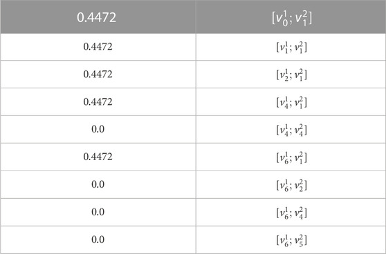
TABLE 3. Principal eigenvector of ${\mathcal{L}}_{\mathrm{0,0}}^{(\mathrm{T})}$ for the CSB of Figure 3. By definition, this is the eigenvector associated with the largest eigenvalue.

There is only one PCH in the bottom layer with respect to the top layer, which is the bottom node $v_1^2$, and its principal cross-hubness is 2.2360.

Interestingly, the number of SCHs that appear for a given eigenvalue tend to vary dramatically with respect to the smallest eigenvalues before it eventually decreases or stabilizes at a very low number (see Figure 5; Figure 6). Some cross-hubs may appear at one stage along the spectrum and then disappear at a future stage. This suggests the notion of spectral persistence of cross-hubs. Nodes that emerge the most often or live longer as cross-hubs along the spectrum might be seen as the most central in restructuring the topology of the other complex layers. The further we move away from the smallest non-zero eigenvalue, the more powerful are the nodes that emerge as hubs facilitating communications between aggregations of nodes in the other layer. The emergence of spectral cross-hubs is represented by a horizontal line—spectral persistence bar—running through the indices of the corresponding eigenvalues (Figure 5). The spectral persistence bars corresponding to all SCHs (the spectral bar codes) obtained from ${\mathcal{L}}_{\mathrm{0,0}}^{(\mathrm{T})}$ (resp. ${\mathcal{L}}_{\mathrm{0,0}}^{(\mathrm{B})}$) constitute a signature for all the clustering structures imposed by the bottom (resp. top) layer to the top (resp. bottom) layer.

FIGURE 5

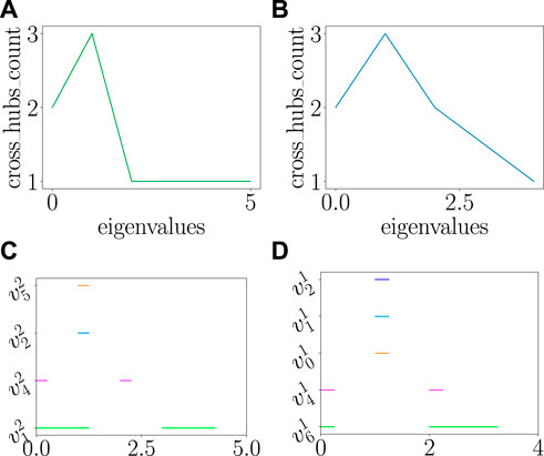
FIGURE 5. Spectral persistence of cross-hubs. Schematic illustrations of the variations in spectral cross-hubs along the eigenvalues and the spectral persistence bars codes for the toy CSB of Figure 3: (A) shows the number of bottom nodes that emerge as spectral cross-hubs with respect to the top layer as a function of the eigenvalues of ${\mathcal{L}}_{\mathrm{0,0}}^{(\mathrm{T})}$, and (B) represents the number of top nodes revealed as spectral cross-hubs with respect to the bottom layer as a function of the eigenvalues of ${\mathcal{L}}_{\mathrm{0,0}}^{(\mathrm{B})}$. (C) and (D) represent the spectral persistence bar codes for ${\mathcal{L}}_{\mathrm{0,0}}^{(\mathrm{T})}$ and ${\mathcal{L}}_{\mathrm{0,0}}^{(\mathrm{B})}$, respectively. For both the top and bottom (0,0) cross-Laplacians, most of the spectral cross-hubs, hence, spectral cross-clusters, emerge during the first stages (smallest eigenvalues), and very few of them survive at later stages; here, only one cross-hub emerges or survives at the largest eigenvalue ($v_1^2$ for ${\mathcal{L}}_{\mathrm{0,0}}^{(\mathrm{T})}$ and $v_6^1$ for ${\mathcal{L}}_{\mathrm{0,0}}^{(\mathrm{B})}$).

FIGURE 6

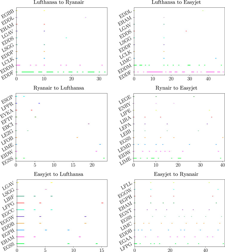
FIGURE 6. Spectral persistent cross-hubs. The spectral persistence bar codes of the six diffusion bicomplexes of the European ATN multiplex. The nodes represent European airports labeled with their ICAO codes (see https://en.wikipedia.org/wiki/ICAO_airport_code). The most persistent cross-hubs correspond to the airports that provide the most efficient correspondences from the first airline network to the second.

5 Experiments on multiplex networks

5.1 Diffusion CSBs

Let $\mathcal{M}$ be a multiplex formed by M graphs Γ^s = (E_s, V), s = 1, … , M. Denoting the vertex set V as an ordered set {1, 2, … , N}, we will write $v_i^s$ to represent the node i in the graph Γ^s, following the same notations we have used for multicomplexes.

For every pair of distinct indices s, t, we define the two-dimensional CSB X^s→t on V × V such that $X_{k,-1}^{s\to t}=\varnothing$ for k ≥ 1, and $X_{-1,k}^{s\to t}$ is the 2-clique complex of the layer indexed by t in the multiplex $\mathcal{M}$; a pair $(v_i^s,v_j^t)\in V\times V$, forms a cross-edge if i < j, and nodes i and j are connected in Γ^s; and a (0,1) crossimplex is a triple $(v_i^s,v_j^t,v_k^t)\in V^3$ such that i is connected to j and k in Γ^s, and j and k are connected in Γ^t, while $X_{\mathrm{1,0}}^{s\to t}=\varnothing$. We call X^s→t the diffusion bicomplex of (layer) s onto t. Notice that by construction, the (0,0) cross-Laplacians of X^s→t are indexed over E_s, while the (0,0) cross-Laplacians of X^t→s are indexed over E_t. This shows that X^s→t and X^t→s are not the same. The diffusion bicomplex X^s→t is a way to look at the topology of Γ^s through the topology of Γ^t; in other words, it diffuses the topology of the former into the topology of the latter.

5.2 Cross-hubs in air transportation networks

We used a subset of the European air transportation network (ATN) dataset (from Cardillo et al., 2013) to construct a three-layered multiplex $\mathcal{M}$ on 450 nodes, each representing a European airport (Wu et al., 2019). The three layer networks Γ¹, Γ², and Γ³ of $\mathcal{M}$ represent the direct flights served by Lufthansa, Ryanair, and easyJet airlines, respectively, that is, intra-layer edges correspond to direct flights between airports served by the corresponding airline. Considering the respective bottom (0,0) cross-Laplacians of the six diffusion bicomplexes X^1→2, X^1→3, X^2→1, X^3→1, X^2→3, and X^3→2, we obtain the spectral persistence bar codes describing the emergence of SCHs for each airline with respect to the others (see Figure 6). The induced SCH rankings are presented in Table 4.

TABLE 4

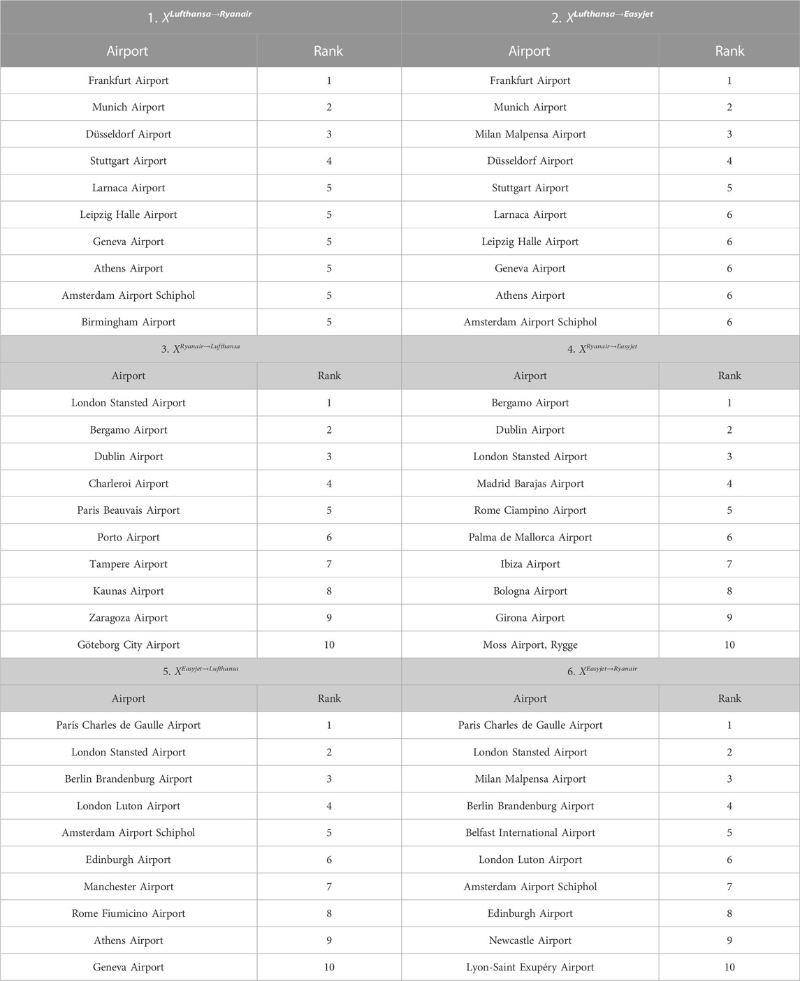
TABLE 4. Ranking of the 10 most persistent SCHs for the diffusion bicomplexes associated with the European air transportation multiplex network.

6 Discussion and conclusion

We have introduced CSM as a generalization of both the notions of simplicial complexes and multilayer networks. We further introduced cross-homology to study their topology and defined the cross-Laplacian operators to detect more structures that are not detected by homology. Our goal here was to set up a mathematical foundation for studying higher-order multilayer complex systems. Nevertheless, through synthetic examples of CSM and applications in multiplex networks, we have shown that our framework provides powerful tools to reveal important topological features in multilayer networks and address questions that would not arise from the standard pairwise-based formalism of multilayer networks. We specially focused on the (0,0) cross-Laplacians to show how their spectra quantify the extent to which nodes in one layer control topological structures in other layers in a multilayer network. Specifically, we saw that the spectra of these matrices allow detection of nodes from one layer that serve as inter-layer connecting hubs for clusters in the other layer; we referred to such nodes as SCHs. Such hubs vary in function of the eigenvalues, and they can be ranked according to their spectral persistence along the spectra of the cross-Laplacians. SCHs obtained from the largest eigenvalues (principal cross-hubs or PCHs) are those that interconnect the most important structures of the other layer. We should note that a PCH is not necessarily spectrally persistent, and two SCHs can be equally persistent but at different ranges of the spectrum. This means that, depending on the applications, some choices need to be made when ranking SCHs based on their spectral persistence. It might be the case that two SCHs persist equally long enough to be considered the most persistent ones, but that one persists through the first quarter of the spectrum, while the other persists through the second quarter of the spectrum so that none of them is PCH.

One can observe that the topological and geometric interpretations given for ${\mathcal{L}}_{\mathrm{0,0}}^{(\mathrm{T})}$ and ${\mathcal{L}}_{\mathrm{0,0}}^{(\mathrm{B})}$ can theoretically be generalized to the higher-order (k, l) cross-Laplacians as well. In other words, the spectra of these operators encode the extent to which higher-order topological structures (edges, triangles, tetrahedrons, and so on) control the emergence of higher-order clustering structures in the other layers. However, in practice, dealing with the higher-order cross-Laplacians could quickly become computationally heavy or infeasible. It would, however, be interesting to see how the (0,1) and (1,1) cross-Laplacians translate in real datasets involving intrinsic intra- and inter-layer triangles and tetrahedrons.

Finally, many recent advances in structural and functional neuroimaging and genomics are based on the analysis of complex network representations of the human brain. The proposed framework will enable us to analyze the intimate relationships between the brain structure, genomics, and functional representations within unified multilayered structures.

7 Methods

7.1 Cones, kites, and the (0,0) cross-Betti numbers

Let $v_j^2$ be a fixed vertex in V₂. A kite from V₁ to $v_j^2$ is an ordered tuple $(v_{i_1}^1,\dots ,v_{i_p}^1)$ of vertices in V₁ such that $\{v_{i_r}^1,v_{i_{r+1}}^1,v_j^2\}\in X_{\mathrm{1,0}}$ for r = 1, … , p − 1. Such an object is denoted as $(v_{i_0}^1,\dots ,v_{i_p}^1\leftarrow v_j^2)$. Beware that the vertices $v_{i_1}^1,\dots ,v_{i_p}^1$ do not need to be pair-wise connected in V₁. We observe the cross-triangles all pointing to $v_j^2$ that are pieced together in the form of an actual kite, as shown in Figure 7. In particular, if $v_j^2$ is the bottom face of a (1,0) cross-triangle $[v_i^1,v_k^1;v_j^2]$, then $(v_i^1,v_k^1\leftarrow v_j^2)$ is a kite. If $(v_{i_1}^1,\dots ,v_{i_p}^1\leftarrow v_j^2)$ is a kite, its boundary is the triple $(v_{i_1}^1,v_{i_p}^1,v_j^2)\in V_1^2\times V_2$. Similarly, given a fixed vertex $v_i^1\in V_1$, one can define a kite from V₂ to $v_i^1$ by a tuple $(v_{j_1}^2,\dots ,v_{j_{p^{\prime }}}^2)$ of vertices in V₂ satisfying the analogous conditions. Such a kite will be denoted as $(v_i^1\to v_{j_1}^2,\dots ,v_{j_{p^{\prime }}}^2)$.

FIGURE 7

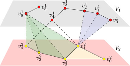
FIGURE 7. Two-dimensional crossimplicial bicomplex containing kites and cones. $(v_0^1,v_1^1,v_2^1)$ is a kite from V1 to $v_1^2\in V_2$ with boundary $(v_0^1,v_2^1,v_1^2)\in V_1^2\times V_2$, and $(v_1^2,v_2^2,v_3^2,v_4^2)$ is a kite from V₂ to $v_6^1\in V_1$ with boundary $(v_6^1,v_1^2,v_4^2)\in V_1\times \in V_2^2$. The tuples $(v_1^2,v_2^2,v_3^2),(v_1^2,v_2^2)$ and $(v_2^2,v_3^2,v_4^2)$ are also kites from V₂ to $v_6^1$. Furthermore, there are three cones with bases in V₁: $(v_2^1,v_4^1,v_1^2)$ is a closed cone with base $(v_2^1,v_4^1)\in V_1$ and vertex $v_1^2\in V_2$, and $(v_4^1,v_6^1,v_1^2)$ is an open cone with base $(v_4^1,v_6^1)\in V_1^2$ and vertex $v_1^2\in V_2$. In addition, $(v_4^1,v_6^1,v_4^2)$ is an open cone with base $(v_4^1,v_6^1)\in V_1^2$ and vertex $v_4^2\in V_2$, and $(v_1^2,v_4^2,v_4^1)\in V_2^2\times V_1$ is a closed cone with base $(v_1^2,v_4^2)\in V_2^2$ and vertex $v_4^1\in V_1$. It follows from Theorem 7.1 that β_0,0 = (3, 1).

It is worth noting that if $(v_{i_1}^1,\dots ,v_{i_p}^1)$ is a kite from V₁ to $v_j^2$, then so is each tuple $(v_{i_r}^1,v_{i_{r+1}}^1,\dots ,v_{i_{r+q}}^1)$ with 1 ≤ r and r + q ≤ p.

By a cross-chain on a kite, we mean one that is a linear combination of the triangles composing the kite; in other words, a cross-chain on the kite $(v_{i_1}^1,\dots ,v_{i_p}^1\leftarrow v_j^2)$ is an element a ∈ C_1,0(X) of the form

$a={\displaystyle \sum _{r=1}^{p-1}}{\gamma }_r\left[v_{i_r}^1,v_{i_{r+1}}^1;v_j^2\right],(13)$

where ${\gamma }_1,\dots ,{\gamma }_{p-1}\in \mathbb{R}$. In a similar fashion, cross-chains on a kite of the form $(v_i^1\to v_{j_1}^2,\dots ,v_{j_{p^{\prime }}}^2)$ are defined.

Now, given a pair $(v_i^1,v_k^1)$ of vertices in the layer V₁ and the vertex $v_j^2\in V_2$, we say that the triple $(v_i^1,v_k^1,v_j^2)\in V_1^2\times V_2$ is a cone with base $(v_i^1,v_k^1)$ and vertex $v_j^2$ if it satisfies the following conditions:

• $v_i^1\sim v_j^2$ and $v_k^1\sim v_j^2$, i.e., $[v_i^1;v_j^2],[v_k^1;v_j^2]\in X_{\mathrm{0,0}}$;

• the triple $(v_i^1,v_k^1,v_j^2)\in V_1^2\times V_2$ is not the boundary of a kite from V₁ to $v_j^2$.

We also say that $(v_i^1,v_k^1,v_j^2)$ is a cone with the base in V₁ and the vertex in V₂. In a similar fashion, one defines a cone with the base in V₂ and the vertex in V₁. We refer to Figure 7 for examples of cones.

An immediate consequence of a triple $(v_i^1,v_k^1,v_j^2)\in V_1^2\times V_2$ being a cone is that the vertices $\{v_i^1,v_k^1,v_j^2\}$ are not (1,0) crossimplex. The vertices $v_i^1$ and $v_k^1$ might, however, be connected by a horizontal path of some length; when we mean that there might be a sequence of vertices $v_{i_0}^1,\dots ,v_{i_p}^1$ in V₁, not all of which form cross-triangles with $v_j^2$, and such that

$v_i^1{⌢}_{}^{(1)}{v}_{i_0}^1{⌢}_{}^{(1)}\cdots {⌢}_{}^{(1)}{v}_{i_p}^1{⌢}_{}^{(1)}{v}_k^1,$

in which case, the cone is said to be closed; it is called open otherwise.

Cones in a crossimplicial bicomplex are classified by the top and bottom (0,0)-cross-homology groups of the bicomplex. Specifically, we have the following topological interpretation of ${\text{H}}_{\mathrm{0,0}}^{(1)}(X)$, ${\text{H}}_{\mathrm{0,0}}^{(2)}(X)$, and hence, the (0,0) cross-Betti numbers.

Theorem 7.1. The (0,0) cross-homology group ${\text{H}}_{\mathrm{0,0}}^{(1)}(X)$ (resp. ${\text{H}}_{\mathrm{0,0}}^{(2)}(X)$) is generated by the cross-homology classes of cones with bases in V₁ and vertices in V₂ (resp. with bases in V₂ and vertices in V₁). Therefore, the (0,0) cross-Betti number ${\beta }_{\mathrm{0,0}}^{(t)}$ counts the cones with bases in V_t, t = 1, 2.

Here, by the cross-homology class of the cone $(v_i^1,v_k^1,v_j^2)\in V_1^2\times V_2$, for instance, we mean the top cross-homology of the (0,0) cross-chain $[v_k^1;v_j^2]-[v_i^1;v_j^2]\in C_{\mathrm{0,0}}(X)$.

Proof. We prove the theorem for ${\text{H}}_{\mathrm{0,0}}^{(1)}(X)$ since the same arguments apply to ${\text{H}}_{\mathrm{0,0}}^{(2)}(X)$. Every cone $(v_i^1,v_k^1,v_j^2)$ defines a non-trivial (0,0) cross-cycle; in other words, the difference of the corresponding cross-edges $[v_i^1;v_j^2]-[v_k^1;v_j^2]\in \ker {\partial }_{\mathrm{0,0}}^{(1)}$. More generally, suppose we are given p cones $(v_{i_1}^1,v_{i_2}^1,v_j^2),(v_{i_2},v_{i_3}^1,v_j^2),\dots ,(v_{i_{p-1}}^1,v_{i_p}^1,v_j^2)$ with bases in V₁ and all with the same vertex $v_j^2\in V_2$. Then, for all real numbers α₁, … , α_p such that ${\sum }_{r=1}^p{\alpha }_r=0$, the cross-chain

$b={\displaystyle \sum _{r=1}^p}{\alpha }_r\left[v_{i_r}^1;v_j^2\right](14)$

is clearly a (0,0) cross-cycle with a non-trivial cross-homology class, i.e., $b\in \ker {\partial }_{\mathrm{0,0}}^{(1)}$ and $b\notin \mathrm{i}\mathrm{m}{\partial }_{\mathrm{1,0}}^{(1)}$. Conversely, let $b^{\prime }\in \ker {\partial }_{\mathrm{0,0}}^{(1)}$. We can write

$b^{\prime }={\displaystyle \sum _{m=1}^M}{\alpha }_m^{\prime }\left[v_{i_m}^1;v_{i_m}^2\right]\in C_{\mathrm{0,0}}\left(X\right),$

so that ${\partial }_{\mathrm{0,0}}^{(1)}(b^{\prime })={\sum }_{m=1}^M{\alpha }_m^{\prime }[v_{i_m}^2]=0$. Then, either all the $v_{i_m}^2$ values are pair-wise different, in which case b′ is the trivial cross-cycle; or there exist p + 1 subsets ${(\{m_{r,1},\dots ,m_{r,M_r}\})}_{r=1}^{p+1}$ of {1, … , M} such that

$v_{i_{m_{r,1}}}^2=v_{i_{m_{r,2}}}^2=\cdots =v_{i_{m_{r,M_r}}}^2,\text{for\hspace{0.17em}}1\le r\le p$

and

$v_{i_{m_{p+1,j}}}^2\ne v_{i_{m_{p+1,j^{\prime }}}}^2,\text{for\hspace{0.17em}all\hspace{0.17em}}j\ne j^{\prime },1\le j,j^{\prime }\le M_{p+1}.$

It follows that

${\displaystyle \sum _{j=1}^{M_r}}{\alpha }_{m_{r,j}}^{\prime }=0,\text{for\hspace{0.17em}each\hspace{0.17em}}r=1,\dots ,p(15)$

and ${\alpha }_{m_{p+1,j}}^{\prime }=0\text{for\hspace{0.17em}all\hspace{0.17em}}j=1,\dots ,M_{p+1}$. Hence, we get the following general expression of a (0,0) cross-cycle:

$b^{\prime }={\displaystyle \sum _{r=1}^p}{\displaystyle \sum _{j=1}^{M_r}}{\alpha }_{m_{r,j}}^{\prime }\left[v_{i_{m_{r,j}}}^1;v_{i_{m_{r,1}}}^2\right],(16)$

where the coefficients satisfy (15). Furthermore, it is straightforward to see that $b^{\prime }\in \mathrm{i}\mathrm{m}{\partial }_{\mathrm{1,0}}^{(1)}$ if, and only if, for each r = 1, … , p, there exists a permutation τ_r of {1, … , M_r} such that

$\left(v_{i_{m_{r,{\tau }_r\left(1\right)}}}^1,\dots ,v_{i_{m_{r,{\tau }_r\left(M_r\right)}}}^1\leftarrow v_{i_{m_{r,1}}}^2\right)$

is a kite. In that case, we get $b^{\prime }={\partial }_{\mathrm{1,0}}^{(1)}(a)$, where

$a={\displaystyle \sum _{r=1}^p}{\displaystyle \sum _{r=1}^{M_r-1}}{\gamma }_{m_{r,j}}\left[v_{i_{m_{r,{\tau }_r\left(j\right)}}}^1,v_{i_{m_{r,{\tau }_r\left(j+1\right)}}}^1;v_{i_{m_{r,1}}}^2\right],(17)$

and where, for r = 1, … , p, the coefficients ${\gamma }_{m_{r,j}}$ are given by

$\left\{\begin{array}{cc}{\gamma }_{m_{r,1}}\hfill & =-{\alpha }_{m_{r,{\tau }_r\left(1\right)}}^{\prime }\hfill \\ {\gamma }_{m_{r,2}}\hfill & =-{\alpha }_{m_{r,{\tau }_r\left(1\right)}}^{\prime }-{\alpha }_{m_{r,{\tau }_r\left(2\right)}}^{\prime }\hfill \\ \hfill & ⋮\hfill \\ {\gamma }_{m_{r,M_r-2}}\hfill & =-{\alpha }_{m_{r,{\tau }_r\left(1\right)}}^{\prime }-{\alpha }_{m_{r,{\tau }_r\left(2\right)}}^{\prime }-\cdots -{\alpha }_{m_{r,{\tau }_r\left(M_r-2\right)}}^{\prime }\hfill \\ {\gamma }_{m_{r,M_r-1}}\hfill & ={\alpha }_{m_{r,{\tau }_r\left(M_2\right)}}^{\prime }.\hfill \end{array}\right.(18)$

This shows that trivial cross-homology classes in ${\text{H}}_{\mathrm{0,0}}^{(1)}(X)$ are given by cross-cycles obtained from cross-chains on kites, i.e., images of sums of cross-chains in the form of (13).

7.2 Inner product, cross-Laplacians, and harmonic cross-forms

We define the following maps on cross-forms:

by the following equations:

${\delta }_{k,l}^{(1)}\varphi \left(\left[a\right]\right)={\displaystyle \sum _{b\in {\partial }_a^{(1)}}}\mathrm{s}\mathrm{g}\mathrm{n}\left(b,{\partial }_a^{(1)}\right)\varphi \left(\left[b\right]\right),\text{and\hspace{0.17em}\hspace{0.17em}}{\delta }_{k,l}^{(2)}\varphi \left(\left[c\right]\right)={\displaystyle \sum _{d\in {\partial }_c^{(2)}}}\mathrm{s}\mathrm{g}\mathrm{n}\left(d,{\partial }_c^{(2)}\right)\varphi \left(\left[d\right]\right),(19)$

for ϕ ∈ C^k,l(X), a ∈ X_k+1,l and c ∈ X_k,l+1.

Now, for each pair of integers (k, l), we choose inner products ⟨⋅,⋅⟩_k,l, ⟨⋅,⋅⟩_k+1,l and ⟨⋅,⋅⟩_k,l+1 on the real vector spaces C^k,l(X), C^k+1,l(X) and C^k,l+1(X), respectively. The adjoint operators ${({\delta }_{k,l}^{(1)})}^{*}:C^{k+1,l}(X)\to C^{k,l}(X)$ and ${({\delta }_{k,l}^{(2)})}^{*}:C^{k,l+1}(X)\to C^{k,l}(X)$ are determined by the following relations:

$\begin{array}{c}\hfill {⟨{\delta }_{k,l}^{(1)}\varphi ,\psi ⟩}_{k+1,l}={⟨\varphi ,{\left({\delta }_{k,l}^{(1)}\right)}^{*}\psi ⟩}_{k,l},\\ \hfill {⟨{\delta }_{k,l}^{(2)}\varphi ,{\psi }^{\prime }⟩}_{k,l+1}={⟨\varphi ,{\left({\delta }_{k,l}^{(2)}\right)}^{*}{\psi }^{\prime }⟩}_{k,l},\end{array}(20)$

for ϕ ∈ C^k,l(X), ψ ∈ C^k+1,l(X), and ψ′ ∈ C^k,l+1(X).

Any weight w on X defines such inner products on cross-forms by the following setting:

${⟨\varphi ,\psi ⟩}_{k,l}≔{\displaystyle \sum _{a\in X_{k,l}}}w\left(a\right)\varphi \left(a\right)\psi \left(a\right),\text{for\hspace{0.17em}\hspace{0.17em}}\varphi ,\psi \in C^{k,l}\left(X\right).(21)$

It can be seen that, with respect to such an inner product, elementary cross-forms form an orthogonal basis. Moreover, given a weight function w and such an inner product, we get the following by simple calculations using (20):

${\left({\delta }_{k,l}^{(1)}\right)}^{*}\varphi \left(\left[a\right]\right)={\displaystyle \sum _{\stackrel{a^{\prime }\in X_{k+1,l}}{a\in {\partial }_{}^{(1)}{a}^{\prime }}}}\frac{w\left(a^{\prime }\right)}{w\left(a\right)}\mathrm{s}\mathrm{g}\mathrm{n}\left(a,{\partial }_{}^{(1)}{a}^{\prime }\right)\varphi \left(\left[a^{\prime }\right]\right),(22)$

for ϕ ∈ C^k+1,l(X), a ∈ X_k,l. In addition, we obtain a similar formula for ${({\delta }_{k,l}^{(2)})}^{*}$.

Definition 7.2. We define the following self-adjoint linear operators on C^k,l(X) for all k, l ≥−1:

• the top-outer (k, l)-cross-Laplacian (or TO-Laplacian of order (k, l)

${\mathcal{L}}_{k,l}^{(\mathrm{T}\mathrm{O})}≔{\left({\delta }_{k,l}^{(1)}\right)}^{*}{\delta }_{k,l}^{(1)},$

• the top-inner (k, l)-cross-Laplacian (or TI-Laplacian of order (k, l)

${\mathcal{L}}_{k,l}^{(\mathrm{T}\mathrm{I})}≔{\delta }_{k-1,l}^{(1)}{\left({\delta }_{k-1,l}^{(1)}\right)}^{*},$

• the top (k, l) cross-Laplacian

${\mathcal{L}}_{k,l}^{(\mathrm{T})}≔{\mathcal{L}}_{k,l}^{(\mathrm{T}\mathrm{O})}+{\mathcal{L}}_{k,l}^{(\mathrm{T}\mathrm{I})},$

• and similarly, the bottom-outer (k, l) cross-Laplacian (BO-Laplacian of order (k, l))

${\mathcal{L}}_{k,l}^{(\mathrm{B}\mathrm{O})}≔{\left({\delta }_{k,l}^{(2)}\right)}^{*}{\delta }_{k,l}^{(2)},$

• the bottom-inner (k, l)-cross-Laplacian (BI-Laplacian)

${\mathcal{L}}_{k,l}^{(\mathrm{B}\mathrm{I})}≔{\delta }_{k,l-1}^{(2)}{\left({\delta }_{k,l-1}^{(2)}\right)}^{*},$

• and the bottom (k, l)-cross-Laplacian

${\mathcal{L}}_{k,l}^{(\mathrm{B})}≔{\mathcal{L}}_{k,l}^{(\mathrm{B}\mathrm{O})}+{\mathcal{L}}_{k,l}^{(\mathrm{B}\mathrm{I})}.$

The null spaces of these operators, defined as the following sub-groups

${}^{(s)}{\mathcal{H}}_{k,l}=\ker {\mathcal{L}}_{k,l}^{(\mathrm{s})}=\left\{\varphi \in C^{k,l}\left(X\right)|{\mathcal{L}}_{k,l}^{(\mathrm{s})}\varphi =0\right\},s=T,B,$

are called the spaces of harmonic top (resp. bottom) cross-forms on X.

There is a one-to-one correspondence between cross-cycle classes and harmonic cross-forms on CSB X. In other words, we have the following group isomorphisms generalizing (Eckmann, 1944; Horak and Jost, 2013).

Lemma 7.3. For s = 1, 2 and for all k, l ≥−1, we have

${\text{H}}_{k,l}^{(s)}\left(X\right)\cong \ker \left({\mathcal{L}}_{k,l}^{(\mathrm{s})}\right),(23)$

where we have used the notations ${\mathcal{L}}_{k,l}^{(1)}={\mathcal{L}}_{k,l}^{(\mathrm{T})}$ and ${\mathcal{L}}_{k,l}^{(2)}={\mathcal{L}}_{k,l}^{(\mathrm{B})}$.

Proof. Let us prove this result for s = 1 (similar arguments apply to s = 2). First, notice that from the identification C_k,l(X) = C^k,l(X), we obtain the following:

${\text{H}}_{k,l}^{(1)}\left(X\right)=\ker \left({\delta }_{k,l}^{(1)}\right)/\mathrm{i}\mathrm{m}\left({\delta }_{k-1,l}^{(1)}\right)\cong \ker \left({\delta }_{k,l}^{(1)}\right)\cap \mathrm{i}\mathrm{m}{\left({\delta }_{k-1,l}^{(1)}\right)}^{\perp },(24)$

and the analog holds for ${\text{H}}_{(2)}^{k,l}(X)$. Moreover, recall from linear algebra that if $E\stackrel{f}{\to }F$ is a linear operator on two vector spaces equipped with inner products, then ker (f*f) = ker f. Indeed, we clearly have ker f ⊂ ker (f*f). Next, if x ∈ ker (f*f), then ${⟨f^{*}fx,y⟩}_E={⟨fx,fy⟩}_F=0$ for all y ∈ E, which implies that x ∈ ker f. In our case, we have ${\delta }_{k,l}^{(1)}{\delta }_{k-1,l}^{(1)}=0$ and ${({\delta }_{k-1,l}^{(1)})}^{*}{({\delta }_{k,l}^{(1)})}^{*}=0$; hence,

$\begin{array}{c}\hfill \mathrm{i}\mathrm{m}\left({\mathcal{L}}_{k,l}^{(\mathrm{T}\mathrm{O})}\right)\subset \mathrm{i}\mathrm{m}{\left({\delta }_{k,l}^{(1)}\right)}^{*}\subset \ker {\left({\delta }_{k-1,l}^{(1)}\right)}^{*}\subset \ker \left({\delta }_{k-1,l}^{(1)}{\left({\delta }_{k-1,l}^{(1)}\right)}^{*}\right)\\ \hfill \mathrm{i}\mathrm{m}\left({\mathcal{L}}_{k,l}^{(\mathrm{T}\mathrm{I})}\right)\subset \mathrm{i}\mathrm{m}\left({\delta }_{k-1,l}^{(1)}\right)\subset \ker \left({\delta }_{k,l}^{(1)}\right)\subset \ker \left({\left({\delta }_{k,l}^{(1)}\right)}^{*}{\delta }_{k,l}^{(1)}\right).\end{array}$

Therefore,

$\begin{array}{c}\ker {\mathcal{L}}_{k,l}^{(\mathrm{T})}=\ker \left({\left({\delta }_{k,l}^{(1)}\right)}^{*}{\delta }_{k,l}^{(1)}\right)\cap \ker \left({\delta }_{k-1,l}^{(1)}{\left({\delta }_{k-1,l}^{(1)}\right)}^{*}\right)\hfill \\ \hfill =\ker \left({\delta }_{k,l}^{(1)}\right)\cap \ker {\left({\delta }_{k-1,l}^{(1)}\right)}^{*}\hfill \\ \hfill \cong \ker \left({\delta }_{k,l}^{(1)}\right)\cap \mathrm{i}\mathrm{m}{\left({\delta }_{k-1,l}^{(1)}\right)}^{\perp },\hfill \end{array}$

and the isomorphism (23) follows from (24).

It follows that the eigenvectors corresponding to the zero eigenvalue of the (k, l) cross-Laplacian ${\mathcal{L}}_{k,l}^{(\mathrm{s})}$ are representative cross-cycles in the homology group ${\text{H}}_{k,l}^{(s)}(X)$. Henceforth, we see that in order to get the dimensions of the cross-homology groups ${\text{H}}_{k,l}^{(s)}(X)$, it suffices to find the eigenspaces corresponding to the zero eigenvalues of ${\mathcal{L}}_{k,l}^{(\mathrm{s})}$. In other words,

${\beta }_{k,l}^{(1)}=\dim \ker {\mathcal{L}}_{k,l}^{(\mathrm{1})},\text{and\hspace{0.17em}}{\beta }_{k,l}^{(2)}=\dim \ker {\mathcal{L}}_{k,l}^{(\mathrm{2})}.(25)$

7.3 Matrix representations

Since the sets X_k,l are finite, the vector spaces C_k,l(X) and C^k,l(X) are finite dimensional, and as we have seen, the latter has the elementary cross-forms e_a, a ∈ X_k,l as orthogonal basis with respect to inner products defined from weight functions. So, the cross-Laplacian operators ${\mathcal{L}}_{k,l}^{(\mathrm{s})},s=T,B$ can be represented as real square matrices of dimension |X_k,l|×|X_k,l| whose entries are indexed by elementary cross-forms e_a. In order to compute these matrix representations, we first need to give their formal expressions as linear operators. Thanks to (22), we get the following for ϕ ∈ C^k,l, a ∈ X_k,l:

$\begin{array}{ll}\hfill {\left({\delta }_{k,l}^{(1)}\right)}^{*}{\delta }_{k,l}^{(1)}\varphi \left(\left[a\right]\right)& ={\displaystyle \sum _{\stackrel{a^{\prime }\in X_{k+1,l}}{a\in {\partial }_{}^{(1)}{a}^{\prime }}}}\frac{w\left(a^{\prime }\right)}{w\left(a\right)}\mathrm{s}\mathrm{g}\mathrm{n}\left(a,{\partial }_a^{(1)}\right)\left({\delta }_{k,l}^{(1)}\varphi \right)\left(\left[a^{\prime }\right]\right)\hfill \\ \hfill & ={\displaystyle \sum _{\stackrel{a^{\prime }\in X_{k+1,l}}{a\in {\partial }_{}^{(1)}{a}^{\prime }}}}\frac{w\left(a^{\prime }\right)}{w\left(a\right)}\mathrm{s}\mathrm{g}\mathrm{n}\left(a,{\partial }_{}^{(1)}{a}^{\prime }\right)\sum _{b\in {\partial }_{}^{(1)}{a}^{\prime }}\mathrm{s}\mathrm{g}\mathrm{n}\left(b,{\partial }_{}^{(1)}{a}^{\prime }\right)\varphi \left(\left[b\right]\right)\hfill \\ \hfill & ={\displaystyle \sum _{\stackrel{a^{\prime }\in X_{k+1,l}}{a\in {\partial }_{}^{(1)}{a}^{\prime }}}}\frac{w\left(a^{\prime }\right)}{w\left(a\right)}\mathrm{s}\mathrm{g}\mathrm{n}\left(a,{\delta }_{}^{(1)}{a}^{\prime }\right)\left[\mathrm{s}\mathrm{g}\mathrm{n}\left(a,{\partial }_{}^{(1)}{a}^{\prime }\right)\varphi \left(\left[a\right]\right)+{\displaystyle \sum _{b\in {\partial }_{}^{(1)}{a}^{\prime },b\ne a}}\mathrm{s}\mathrm{g}\mathrm{n}\left(b,{\partial }_{}^{(1)}{a}^{\prime }\right)\varphi \left(\left[b\right]\right)\right]\hfill \\ \hfill & ={\displaystyle \sum _{\stackrel{a^{\prime }\in X_{k+1,l}}{a\in {\partial }_{}^{(1)}{a}^{\prime }}}}\frac{w\left(a^{\prime }\right)}{w\left(a\right)}\left[\varphi \left(\left[a\right]\right)+{\displaystyle \sum _{b\in {\partial }_{}^{(1)}{a}^{\prime },a\ne b}}\mathrm{s}\mathrm{g}\mathrm{n}\left(a,{\partial }_{}^{(1)}{a}^{\prime }\right)\mathrm{s}\mathrm{g}\mathrm{n}\left(b,{\partial }_{}^{(1)}{a}^{\prime }\right)\varphi \left(\left[b\right]\right)\right],\hfill \end{array}$

and

$\begin{array}{ll}\hfill {\delta }_{k-1,l}^{(1)}{\left({\delta }_{k-1,l}^{(1)}\right)}^{*}\varphi \left(\left[a\right]\right)& ={\displaystyle \sum _{\stackrel{c\in X_{k-1,l}}{c\in {\partial }_a^{(1)}}}}\mathrm{s}\mathrm{g}\mathrm{n}\left(c,{\partial }_{}^{(1)}{a}^{\prime }\right){\displaystyle \sum _{\stackrel{a^{\prime }\in X_{k,l}}{c\in {\partial }_{}^{(1)}{a}^{\prime }}}}\frac{w\left(a^{\prime }\right)}{w\left(c\right)}\mathrm{s}\mathrm{g}\mathrm{n}\left(c,{\partial }_{}^{(1)}{a}^{\prime }\right)\varphi \left(\left[a^{\prime }\right]\right)\hfill \\ \hfill & ={\displaystyle \sum _{\stackrel{c\in X_{k-1,l}}{c\in {\partial }_a^{(1)}}}}\mathrm{s}\mathrm{g}\mathrm{n}\left(c,{\partial }_a^{(1)}\right)\left[\frac{w\left(a\right)}{w\left(c\right)}\mathrm{s}\mathrm{g}\mathrm{n}\left(c,{\partial }_a^{(1)}\right)\varphi \left(\left[a\right]\right)\right.\hfill \\ \hfill & +\left.{\displaystyle \sum _{\stackrel{c\in {\partial }_{}^{(1)}{a}^{\prime }}{a\ne a^{\prime }}}}\frac{w\left(a^{\prime }\right)}{w\left(c\right)}\mathrm{s}\mathrm{g}\mathrm{n}\left(c,{\partial }_{}^{(1)}{a}^{\prime }\right)\varphi \left(\left[a^{\prime }\right]\right)\right]\hfill \\ \hfill & ={\displaystyle \sum _{\stackrel{c\in X_{k-1,l}}{c\in {\partial }_a^{(1)}}}}\frac{w\left(a\right)}{w\left(c\right)}\varphi \left(\left[a\right]\right)+{\displaystyle \sum _{\stackrel{c\in X_{k-1,l},a^{\prime }\in X_{k,l}}{c={\partial }_{}^{(1)}{a}^{\prime }\cap {\partial }_a^{(1)}}}}\frac{w\left(a^{\prime }\right)}{w\left(c\right)}\mathrm{s}\mathrm{g}\mathrm{n}\left(c,{\partial }_a^{(1)}\right)\mathrm{s}\mathrm{g}\mathrm{n}\left(c,{\partial }_{}^{(1)}{a}^{\prime }\right)\varphi \left(\left[a^{\prime }\right]\right).\hfill \end{array}$

In particular, when ϕ is an elementary cross-form e_b, b ∈ X_k,l, we obtain the following:

${\mathcal{L}}_{k,l}^{(\mathrm{T}\mathrm{O})}{e}_b\left(\left[a\right]\right)=\left\{\begin{array}{cc}\frac{1}{w\left(a\right)}{\mathrm{deg}}_{TO}\left(a\right),\hfill & \text{if\hspace{0.17em}}a=b,\hfill \\ \hfill \\ -\frac{w\left(c\right)}{w\left(a\right)},\hfill & \text{if\hspace{0.17em}\hspace{0.17em}}a\ne b\text{and\hspace{0.17em}\hspace{0.17em}}a{⌢}_c^{(1)}b,\hfill \\ \hfill & \text{and\hspace{0.17em}have\hspace{0.17em}same\hspace{0.17em}orientation},\hfill \\ \hfill \\ \frac{w\left(c\right)}{w\left(a\right)},\hfill & \text{if\hspace{0.17em}\hspace{0.17em}}a\ne b\text{and\hspace{0.17em}\hspace{0.17em}}a{⌢}_c^{(1)}b,\hfill \\ \hfill & \text{and\hspace{0.17em}have\hspace{0.17em}opposite\hspace{0.17em}orientations},\hfill \\ \hfill \\ 0,\hfill & \text{otherwise\hspace{0.17em}},\hfill \end{array}\right.$

and

${\mathcal{L}}_{k,l}^{(\mathrm{T}\mathrm{I})}{e}_b\left(\left[a\right]\right)=\left\{\begin{array}{cc}w\left(a\right){\mathrm{deg}}_{TI}\left(a\right),\hfill & \text{if\hspace{0.17em}}a=b,\hfill \\ \hfill \\ \frac{w\left(b\right)}{w\left(d\right)},\hfill & \text{if\hspace{0.17em}}a\ne b\text{and\hspace{0.17em}}a{⌣}_{(1)}^{d}b,\hfill \\ \hfill & \text{and\hspace{0.17em}have\hspace{0.17em}same\hspace{0.17em}orientation},\hfill \\ \hfill \\ -\frac{w\left(b\right)}{w\left(d\right)},\hfill & \text{if\hspace{0.17em}}a\ne b\text{and\hspace{0.17em}}a{⌣}_{(1)}^{d}b\hfill \\ \hfill & \text{and\hspace{0.17em}have\hspace{0.17em}opposite\hspace{0.17em}\hspace{0.17em}orientations},\hfill \\ \hfill \\ 0,\hfill & \text{otherwise\hspace{0.17em}}.\hfill \end{array}\right.$

It follows that the (e_a, e_b)-th entry of the matrix representation of the top (k, l) cross-Laplacian ${\mathcal{L}}_{k,l}^{(\mathrm{T})}$ with respect to the inner product defined from the weight function w is given by the following:

${\left({\mathcal{L}}_{k,l}^{(T)}\right)}_{e_a,e_b}=\left\{\begin{array}{cc}\frac{1}{w\left(a\right)}{\mathrm{deg}}_{TO}\left(a\right)+w\left(a\right){\mathrm{deg}}_{TI}\left(a\right),\hfill & \text{if\hspace{0.17em}}a=b,\hfill \\ \hfill \\ \frac{w\left(b\right)}{w\left(d\right)}-\frac{w\left(c\right)}{w\left(a\right)},\hfill & \text{if\hspace{0.17em}\hspace{0.17em}}a\ne b,a{⌢}_c^{(1)}b\text{and\hspace{0.17em}}a{⌣}_{(1)}^{d}b,\hfill \\ \hfill & \text{and\hspace{0.17em}have\hspace{0.17em}same\hspace{0.17em}orientation}\hfill \\ \hfill \\ \frac{w\left(c\right)}{w\left(a\right)}-\frac{w\left(b\right)}{w\left(d\right)},\hfill & \text{if\hspace{0.17em}\hspace{0.17em}}a\ne b,a{⌢}_c^{(1)}b\text{and\hspace{0.17em}}a{⌣}_{(1)}^{d}b,\hfill \\ \hfill & \text{and\hspace{0.17em}have\hspace{0.17em}opposite\hspace{0.17em}orientations}\hfill \\ \hfill \\ \frac{w\left(b\right)}{w\left(d\right)},\hfill & \text{if\hspace{0.17em}}a\ne b,a{⌣}_{(1)}^{d}b,\text{same\hspace{0.17em}orientation},\hfill \\ \hfill & \text{and\hspace{0.17em}not\hspace{0.17em}\hspace{0.17em}top}-\text{outer\hspace{0.17em}\hspace{0.17em}adjacent},\hfill \\ \hfill \\ -\frac{w\left(b\right)}{w\left(d\right)},\hfill & \text{if\hspace{0.17em}}a\ne b,a{⌣}_{(1)}^{d}b,\text{opposite\hspace{0.17em}orientations},\hfill \\ \hfill & \text{and\hspace{0.17em}not\hspace{0.17em}\hspace{0.17em}top}-\text{outer\hspace{0.17em}\hspace{0.17em}adjacent},\hfill \\ \hfill \\ 0,\hfill & \text{otherwise\hspace{0.17em}}.\hfill \end{array}\right.(26)$

It is clear that we get similar matrix representation for the bottom (k, l) cross-Laplacian ${\mathcal{L}}_{k,l}^{(\mathrm{B})}$.

Data availability statement

Publicly available datasets were analyzed in this study. These data can be found at: http://complex.unizar.es/∼atnmultiplex/.

Author contributions

EM: conceptualization, data curation, formal analysis, investigation, methodology, software, validation, visualization, writing–original draft, and writing–review and editing. OA: writing–review and editing. HB: Funding acquisition, investigation, project administration, resources, supervision, validation, visualization, and writing–review and editing.

Funding

The author(s) declare financial support was received for the research, authorship, and/or publication of this article. This work was supported by the Natural Sciences and Engineering Research Council of Canada through the CRC grant NC0981.

Acknowledgments

The code used for visualizations and computations will be made available upon request.

Conflict of interest

The authors declare that the research was conducted in the absence of any commercial or financial relationships that could be construed as a potential conflict of interest.

Publisher’s note

All claims expressed in this article are solely those of the authors and do not necessarily represent those of their affiliated organizations, or those of the publisher, the editors, and the reviewers. Any product that may be evaluated in this article, or claim that may be made by its manufacturer, is not guaranteed or endorsed by the publisher.

References

Benson, A. R., Gleich, D. F., and Leskovec, J. (2016). Higher-order organization of complex networks. Science 353 (6295), 163–166. doi:10.1126/science.aad9029

PubMed Abstract | CrossRef Full Text | Google Scholar

Bianconi, G. (2021). Higher-order networks. Cambridge University Press.

Google Scholar

Boccaletti, S., Bianconi, G., Criado, R., Del Genio, C. I., Gómez-Gardenes, J., Romance, M., et al. (2014). The structure and dynamics of multilayer networks. Phys. Rep. 544 (1), 1–122. doi:10.1016/j.physrep.2014.07.001

PubMed Abstract | CrossRef Full Text | Google Scholar

Cardillo, A., Gómez-Gardenes, J., Zanin, M., Romance, M., Papo, D., Pozo, F. d., et al. (2013). Emergence of network features from multiplexity. Sci. Rep. 3 (1), 1344–1346. doi:10.1038/srep01344

PubMed Abstract | CrossRef Full Text | Google Scholar

De Domenico, M., Solé-Ribalta, A., Cozzo, E., Kivelä, M., Moreno, Y., Porter, M. A., et al. (2013). Mathematical formulation of multilayer networks. Phys. Rev. X 3 (4), 041022. doi:10.1103/physrevx.3.041022

CrossRef Full Text | Google Scholar

Eckmann, B. (1944). Harmonische funktionen und randwertaufgaben in einem komplex. Comment. Math. Helvetici 17, 240–255. doi:10.1007/bf02566245

CrossRef Full Text | Google Scholar

Flores, J., and Romance, M. (2018). On eigenvector-like centralities for temporal networks: discrete vs. continuous time scales. J. Comput. Appl. Math. 330, 1041–1051. doi:10.1016/j.cam.2017.05.019

CrossRef Full Text | Google Scholar

Fortunato, S., and Hric, D. (2016). Community detection in networks: a user guide. Phys. Rep. 659, 1–44. doi:10.1016/j.physrep.2016.09.002

CrossRef Full Text | Google Scholar

Goerss, P. G., and Jardine, J. F. (2009). Simplicial homotopy theory. Springer Science and Business Media.

Google Scholar

Griffa, A., Ricaud, B., Benzi, K., Bresson, X., Daducci, A., Vandergheynst, P., et al. (2017). Transient networks of spatio-temporal connectivity map communication pathways in brain functional systems. NeuroImage 155, 490–502. doi:10.1016/j.neuroimage.2017.04.015

PubMed Abstract | CrossRef Full Text | Google Scholar

Hatcher, A. (2000). Algebraic topology. Cambridge: Cambridge Univ. Press.

Google Scholar

Horak, D., and Jost, J. (2013). Spectra of combinatorial laplace operators on simplicial complexes. Adv. Math. 244, 303–336. doi:10.1016/j.aim.2013.05.007

CrossRef Full Text | Google Scholar

Iacopini, I., Petri, G., Barrat, A., and Latora, V. (2019). Simplicial models of social contagion. Nat. Commun. 10 (1), 2485. doi:10.1038/s41467-019-10431-6

PubMed Abstract | CrossRef Full Text | Google Scholar

Kivelä, M., Arenas, A., Barthelemy, M., Gleeson, J. P., Moreno, Y., and Porter, M. A. (2014). Multilayer networks. J. complex Netw. 2 (3), 203–271. doi:10.1093/comnet/cnu016

CrossRef Full Text | Google Scholar

Lim, L.-H. (2020). Hodge laplacians on graphs. SIAM Rev. 62, 685–715. doi:10.1137/18m1223101

CrossRef Full Text | Google Scholar

Liu, X., Maiorino, E., Halu, A., Glass, K., Prasad, R. B., Loscalzo, J., et al. (2020). Robustness and lethality in multilayer biological molecular networks. Nat. Commun. 11 (1), 6043. doi:10.1038/s41467-020-19841-3

PubMed Abstract | CrossRef Full Text | Google Scholar

Lotito, Q. F., Musciotto, F., Montresor, A., and Battiston, F. (2022). Higher-order motif analysis in hypergraphs. Commun. Phys. 5 (1), 79. doi:10.1038/s42005-022-00858-7

CrossRef Full Text | Google Scholar

Lucas, M., Cencetti, G., and Battiston, F. (2020). Multiorder laplacian for synchronization in higher-order networks. Phys. Rev. Res. 2 (3), 033410. doi:10.1103/physrevresearch.2.033410

CrossRef Full Text | Google Scholar

Mac Lane, S. (1963). Homology. Grundlehren der mathematischen Wissenschaften in Einzeldarstellungen mit besonderer Berücksichtigung der Anwendungsgebiete. Springer Berlin, Heidelberg: Academic Press. doi:10.1007/978-3-642-62029-4

CrossRef Full Text | Google Scholar

Majhi, S., Perc, M., and Ghosh, D. (2022). Dynamics on higher-order networks: a review. J. R. Soc. Interface 19 (188), 20220043. doi:10.1098/rsif.2022.0043

PubMed Abstract | CrossRef Full Text | Google Scholar

Mandke, K., Meier, J., Brookes, M. J., O’Dea, R. D., Van Mieghem, P., Stam, C. J., et al. (2018). Comparing multilayer brain networks between groups: introducing graph metrics and recommendations. NeuroImage 166, 371–384. doi:10.1016/j.neuroimage.2017.11.016

PubMed Abstract | CrossRef Full Text | Google Scholar

Moerdijk, I. (1989). Bisimplicial sets and the group-completion theorem. Dordrecht: Springer Netherlands, 225–240.

CrossRef Full Text | Google Scholar

Newman, M. E. (2003). The structure and function of complex networks. SIAM Rev. 45 (2), 167–256. doi:10.1137/s003614450342480

CrossRef Full Text | Google Scholar

Pedersen, M., Zalesky, A., Omidvarnia, A., and Jackson, G. D. (2018). Multilayer network switching rate predicts brain performance. Proc. Natl. Acad. Sci. 115 (52), 13376–13381. doi:10.1073/pnas.1814785115

PubMed Abstract | CrossRef Full Text | Google Scholar

Pilosof, S., Porter, M. A., Pascual, M., and Kéfi, S. (2017). The multilayer nature of ecological networks. Nat. Ecol. Evol. 1 (4), 0101. doi:10.1038/s41559-017-0101

PubMed Abstract | CrossRef Full Text | Google Scholar

Sánchez-García, R. J., Cozzo, E., and Moreno, Y. (2014). Dimensionality reduction and spectral properties of multilayer networks. Phys. Rev. E 89 (5), 052815. doi:10.1103/physreve.89.052815

CrossRef Full Text | Google Scholar

Schaub, M. T., Benson, A. R., Horn, P., Lippner, G., and Jadbabaie, A. (2020). Random walks on simplicial complexes and the normalized hodge 1-laplacian. SIAM Rev. 62 (2), 353–391. doi:10.1137/18m1201019

CrossRef Full Text | Google Scholar

Shi, D., Chen, Z., Sun, X., Chen, Q., Ma, C., Lou, Y., et al. (2021). Computing cliques and cavities in networks. Commun. Phys. 4, 249. doi:10.1038/s42005-021-00748-4

CrossRef Full Text | Google Scholar

Solá, L., Romance, M., Criado, R., Flores, J., García del Amo, A., and Boccaletti, S. (2013). Eigenvector centrality of nodes in multiplex networks. Chaos (Woodbury, N.Y.) 23, 033131. doi:10.1063/1.4818544

PubMed Abstract | CrossRef Full Text | Google Scholar

Timóteo, S., Correia, M., Rodríguez-Echeverría, S., Freitas, H., and Heleno, R. (2018). Multilayer networks reveal the spatial structure of seed-dispersal interactions across the great rift landscapes. Nat. Commun. 9 (1), 140. doi:10.1038/s41467-017-02658-y

PubMed Abstract | CrossRef Full Text | Google Scholar

Vasilyeva, E., Kozlov, A., Alfaro-Bittner, K., Musatov, D., Raigorodskii, A., Perc, M., et al. (2021). Multilayer representation of collaboration networks with higher-order interactions. Sci. Rep. 11, 5666. doi:10.1038/s41598-021-85133-5

PubMed Abstract | CrossRef Full Text | Google Scholar

Wu, M., He, S., Zhang, Y., Chen, J., Sun, Y., Liu, Y.-Y., et al. (2019). A tensor-based framework for studying eigenvector multicentrality in multilayer networks. Proc. Natl. Acad. Sci. 116, 15407–15413. doi:10.1073/pnas.1801378116

PubMed Abstract | CrossRef Full Text | Google Scholar

Young, J.-G., Petri, G., and Peixoto, T. P. (2021). Hypergraph reconstruction from network data. Commun. Phys. 4 (1), 135. doi:10.1038/s42005-021-00637-w

CrossRef Full Text | Google Scholar

Yuvaraj, M., Dey, A. K., Lyubchich, V., Gel, Y. R., and Poor, H. V. (2021). Topological clustering of multilayer networks. Proc. Natl. Acad. Sci. U. S. A. 118 (21), e2019994118. doi:10.1073/pnas.2019994118

PubMed Abstract | CrossRef Full Text | Google Scholar