Traces of tricritical dynamics beyond SSB in finite-size systems undergoing second-order phase transition: the case of the 3D Ising model

In finite-size thermal systems that exhibit second-order phase transition, the fluctuations of the order parameter ${\varphi }_n$ obey type I intermittent dynamics at their pseudocritical temperature $T_{pc}$. Moreover, as recently demonstrated, spontaneous symmetry breaking (SSB) is gradually completed as temperature is reduced until reaching an SSB completion temperature, $T_{SSB}$. Within this temperature zone, ${\varphi }_n$ obey the dynamics of critical intermittency. This behavior has also been observed in pre-seismic fracture-induced electromagnetic emissions (FEME) of the MHz band—a real-world finite-size system undergoing a second-order phase transition. Interestingly, MHz FEME has recently been found to consistently present indications of tricritical dynamics after the SSB. We examine here whether this could also be true for a finite-size thermal system. We conduct a numerical experiment for the 3D Ising model at different temperatures by gradually reducing temperature beyond SSB and analyze order parameter fluctuations using the method of critical fluctuations (MCF) and a recently introduced wavelet-based method for detecting scaling behavior in noisy experimental data. Our results reveal that power-laws still exist within a very narrow zone of temperatures right after SSB completion for the 3D Ising model. These power-laws are shown to be compatible with another form of intermittency that determines the dynamics of the order parameter fluctuations close to the Griffiths tricritical point. As a possible interpretation of this finding, we suggest that our results imply that 3D Ising presents, just below $T_{SSB}$, an imprint approaching the Griffiths tricritical point from the second-order phase transition line.

1 Introduction

Thermal systems that exhibit second-order phase transitions and spontaneous symmetry breaking (SSB) present typical features of complex systems, such as criticality, long-range correlations, scale-invariance, universality, and order emergence (Stanley, 1971; Goldenfeld, 1992; Solé et al., 1996; Fisher, 1998; Stanley, 1999; Folk and Moser, 2006; Brézin, 2010; Landau, and Lifshitz, 2013; West, 2017; Pathria and Beale, 2022; San Miguel, 2023; Quintana and Berger, 2023; Liu et al., 2023). Near the critical point, they exhibit scale-invariance and long-range correlations that span the whole system. The SSB phenomenon—the breaking of symmetry without the application of an external field—is particularly important since it is a typical order emergence case due to the collective behavior of system constituents which cannot be predicted solely from the microscopic laws governing the system (Anderson, 1972; Goldenfeld, 1992; Landau, and Lifshitz, 2013; Minganti et al., 2021).

For thermal systems of infinite size undergoing a second-order phase transition, the established theory for the SSB phenomenon can be expressed through the notion of Ginzburg–Landau (G-L) free energy, using terms up to fourth-order (${\varphi }^4$ theory) (Huang, 1987; Ryder, 1985; Goldenfeld, 1992; Kaku, 1993; Landau, and Lifshitz, 2013). When the temperature (control parameter for thermal systems) is equal to the critical temperature ($T=T_c$), the system is at its symmetrical phase. In the symmetrical phase, G-L free energy presents a single minimum at a particular value of the order parameter. As soon as the temperature drops below the critical temperature, a degenerate set of minima emerges, inducing the spontaneous breaking of the symmetry. For infinite-size systems, an important feature to note is the lack of communication between the G-L free-energy degenerate minima (which are disconnected). Therefore, in this case, the equilibrated system must choose a specific free-energy minimum for $T<T_c$ (Beekman et al., 2019) where SSB is exact and holds for any temperature below $T_c$. Since a high number of the order parameter values are attracted around the G-L free-energy minimum/minima (fixed point), the SSB phenomenon is reflected as follows to the distribution of the order parameter values. At the critical temperature ($T=T_c$), the distribution is unimodal (one lobe), whereas for any $T<T_c$ the distribution becomes bimodal (two lobes) and these two lobes are completely separated.

Although ${\varphi }^4$ theory is a cornerstone for understanding second-order transitions, it is well-known that for finite-size systems, a number of deviations from ${\varphi }^4$ theory is observed (Stanley, 1971; Fisher and Barber, 1972; Barber, 1983; Binder, 1992; Goldenfeld, 1992; Brézin and Zinn-Justin, 1985; Brankov et al., 2000; Pelissetto and Vicari, 2002; Hasenbusch et al., 2008; Hasenbusch, 2010; Fytas et al., 2023). Specifically, it has recently been found regarding SSB (Diakonos et al., 2022; Contoyiannis et al., 2021) that a temperature zone which presents interesting properties, termed the “hysteresis zone” (or “transition zone,” or “SSB zone”) (Diakonos et al., 2022; Contoyiannis et al., 2021), emerges below the pseudocritical temperature ($T_{pc}$). There is a specific temperature, which has been termed “temperature of spontaneous symmetry breaking” or “SSB completion temperature” (Diakonos et al., 2022; Contoyiannis et al., 2021) T_SSB < T_pc, at which SSB is achieved (complete separation of the two lobes of the order parameter fluctuations’ distribution). Importantly, for temperatures within the “hysteresis zone”, i.e., for T_SSB < T < T_pc, the two lobes, although exist, are not fully separated. This practically means that the second-order phase transition critical point survives inside this zone, even though the mathematical symmetry in the G-L free energy is broken for T < T_pc. The critical point appears for the last time just before T_SSB is reached. This behavior of finite-size thermal systems explains the presence of power-laws compatible with critical dynamics for as long as the two lobes are not completely separated.

The specific temperature zone properties were studied in detail in Diakonos et al. (2022) and Contoyiannis et al. (2021). As demonstrated in the latter, the width $\Delta T=T_{pc}-T_{SSB}$ depends upon the length of the system through a power-law of the form $\Delta T\sim d^{-m}$ ($m\ge 1$), where $d$ is the length of the lattice. Specifically, it was found that ${\Delta T}_{2D}\sim d^{-1}$ and ${\Delta T}_{3D}\sim d^{-\frac{14}{9}}$ for the 2D and 3D Ising models, respectively (Diakonos et al., 2022). Therefore, the smaller the system size, the wider the zone. Consequently, for an infinite-size system ($d\to \infty$), the zone $\Delta T$ vanishes ($\underset{d\to \infty }{\lim }\Delta T=0$). Therefore, at the limit of a system of infinite size, SSB is achieved for any $T<T_c$; this is in perfect agreement with the aforementioned established theory for SSB in terms of G-L ${\varphi }^4$ theory.

The above hysteresis zone behavior of finite-size thermal systems has also been identified in a number of real-world finite-size systems, including pre-seismic fracture-induced electromagnetic emissions (FEME) of the MHz band (Contoyiannis and Potirakis, 2018; Potirakis et al., 2023). Interestingly, although not published yet, indications of power-laws compatible with tricritical dynamics have recently been found to consistently appear after SSB in the analysis of the MHz FEME time series. Specifically, the following sequence has been observed: power-laws compatible with critical dynamics, followed by indications of SSB gradual completion as in finite-size thermal systems, followed by power-laws compatible with tricritical dynamics (e.g. Contoyiannis et al., 2025). The pre-seismic MHz FEME has been found to behave analogously to a thermal system undergoing second-order phase transition in equilibrium, where the amplitude of MHz FEME plays the role of the order parameter and the role of control parameter could be played by stress, strain, or time (Contoyiannis and Potirakis, 2018). Therefore, the above observed sequence leads to the following reasonable questions. Is it possible that such a sequence can be observed in finite-size thermal systems too? If so, how can it be explained? These questions were the motivation for the present study. Therefore, the purpose here is to investigate what happens to finite-size thermal systems for temperatures $T<T_{SSB}$ in a region very close to $T_{SSB}$ using the 3D Ising model. Specifically, this study focuses on checking whether power-laws are present beyond SSB for the 3D Ising model, in contrast to what is expected for infinite systems undergoing second-order phase transition, and examining whether these are compatible to tricritical dynamics.

Our results do verify that the 3D Ising model presents power-laws compatible with tricritical dynamics just below $T_{SSB}$, whereas this behavior is not observed for lower temperatures. An interpretation of this behavior is provided through the so-called Griffiths tricritical point (Huang, 1987). It is known from the theory of critical phenomena (Huang, 1987) that there is a region where a second-order phase transition, characterized by critical behavior, meets one of the first-order, characterized by an abrupt change. This is accomplished around the Griffiths tricritical point. Our results imply that 3D Ising presents, just below $T_{SSB}$, an imprint of approaching the Griffiths tricritical point from the second-order phase transition line.

The rest of the study is organized as follows. In “Materials and Methods” (Section 2), we briefly present key notions of second-order phase transition and the Griffiths tricritical point in terms of G-L free energy (${\varphi }^4$ and ${\varphi }^6$ theories, respectively), a critical intermittency type I map, and a tricritical intermittency map (Section 2.1), as well as the time-series analysis methodology for the identification of power-laws compatible with critical and tricritical dynamics (Section 2.2). In “Results” (Section 3), we present key information about the 3D Ising model (Section 3.1), the results of a numerical experiment studying 3D Ising at different temperatures ($T\approx T_{pc}$, $T_{SSB}<T<T_{pc}$, a temperature just below $T_{SSB}$, and even lower temperatures) (Section 3.2), and the results of the power-law analysis of the time series obtained (Section 3.3). In Section 4, we discuss our results and provide an interpretation in terms of critical and tricritical intermittency. Section 5 presents the conclusions.

2 Materials and methods

2.1 Second-order phase transition, Griffiths tricritical point, and critical and tricritical intermittency

Infinite-size thermal systems undergoing a second-order phase transition can be studied within the Landau approach for describing critical phenomena through the notion of Ginzburg–Landau (G-L) free energy, $U\left(\varphi \right)$, using terms up to fourth order (${\varphi }^4$ theory) (Huang, 1987; Ryder, 1985; Kaku, 1993):

$U\left(\varphi \right)=a{\varphi }^2+b{\varphi }^4,(1)$

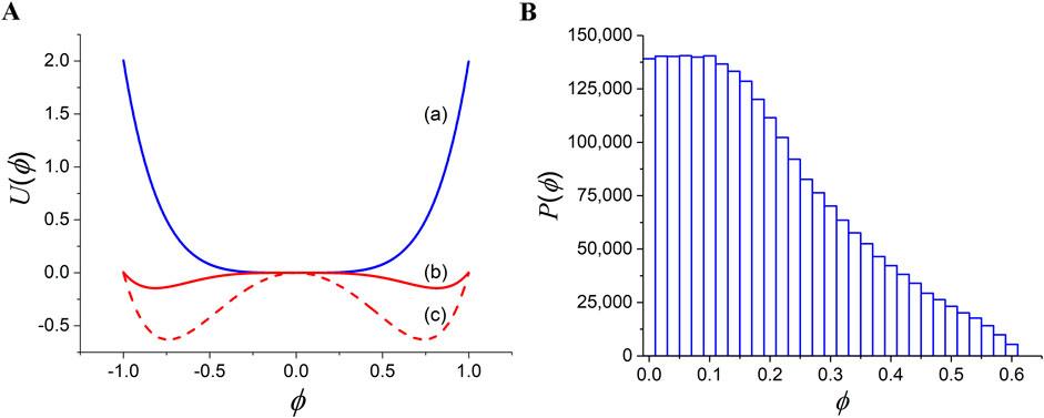
where $\varphi$ denotes the order parameter, and for the coefficients of Equation 1 holds $a,b>0$ for the symmetrical phase when the temperature (control parameter) is equal to critical temperature ($T=T_c$) (blue curve in Figure 1A), and $a<0,b>0$ for the broken symmetry phase for any $T<T_c$ (red and red dashed curves in Figure 1A).

Figure 1

Figure 1. (A) G-L free energy $U\left(\varphi \right)$ vs. the order parameter $\varphi$ for the second-order transition of a thermal system of infinite size: (a) symmetrical phase (achieved for $T=T_c$); (b) SSB (for an arbitrarily selected $T=T_1<T_c$); (c) SSB (for another arbitrarily selected $T=T_2<T_1<T_c$). (B) Distribution of the order parameter $\varphi$ values produced by the critical intermittent map of Equation 2 (only the positive ones are shown).

As shown in Figure 1A, G-L free energy in the symmetrical phase presents a single minimum at a particular value of the order parameter ${\varphi }_0=0$. In addition, as soon as the temperature drops below the critical temperature, a degenerate set of minima emerges, inducing the spontaneous breaking of the symmetry. In the case of an infinite-size system, an important feature to note is the lack of communication between the free-energy degenerate minima (the free-energy minima are disconnected). Therefore in this case, the equilibrated system has to choose a specific free-energy minimum for $T<T_c$ (Beekman et al., 2019) i.e., SSB is exact and holds for any temperature below $T_c$.

It has been demonstrated that the fluctuations of the order parameter at the critical state, simulated by single-spin flip dynamics, are mathematically described by the critical intermittency type I map (Contoyiannis and Diakonos, 2000; Contoyiannis et al., 2002):

${\varphi }_{n+1}={\varphi }_n+u_1{\varphi }_n^{z_1}+{\epsilon }_n,(2)$

where ${\varphi }_n$ is the $n$th sample of the scaled order parameter, $u_1>0$ is a coupling parameter, $z_1>0$ stands for a characteristic exponent, and the shift parameter ${\epsilon }_n$ stands for the non-universal stochastic noise necessary for the creation of ergodicity. As shown in Contoyiannis and Diakonos (2000) and Contoyiannis et al. (2002), if ${\varphi }_n$ denotes the fluctuations of the order parameter, then the exponent $z_1$ is connected to the isothermal critical exponent $\delta$ with the relation $z_1=\delta +1$. Note that in case that the exponent is not an integer, the nonlinear term should be used as $+u_1{\left|{\varphi }_n\right|}^{z_1}$.

The phenomenon of intermittency (Schuster and Just, 2005) consists of alternating segments of small fluctuations delimited by an amplitude interval known as the laminar region, interrupted by chaotic bursts; the waiting times within the laminar region are called “laminar lengths”($L$). Note that the 1D map of Equation 2 acts as a repellor that produces intermittent fluctuations of the order parameter. Specifically, its fixed point is zero and its non-linear term ${u_1\varphi }_n^{z_1}$ drives the trajectory away from the laminar region by leading to higher values (Potirakis et al., 2025). In the case of critical intermittency, the distribution of laminar lengths obeys a power-law of the form (Schuster and Just, 2005)

$P\left(L\right)\sim L^{-p},(3)$

with the condition that (Contoyiannis et al., 2002)

$p=\frac{z_1}{z_1-1}=\frac{\delta +1}{\delta }=1+\frac{1}{\delta }.(4)$

Given that $\delta >1$ (Huang, 1987), it is expected that the critical exponent values would be $\left.p\in [1,2\right)$. Thus, finding power-laws for the distribution of laminar lengths with exponent $p$ value in the abovementioned interval indicates the existence of criticality (Contoyiannis et al., 2002).

In Figure 1B, we present the distribution of order parameter $\varphi$ when the intermittent map of Equation 2 is run for $5·{10}^6$ iterations, with parameter values $z_1=4,$ $u_1=0.011$, and ${\epsilon }_n\in \left[-0.0175,0.0175\right]$ (Contoyiannis and Diakonos, 2007). This distribution corresponds to the symmetrical phase of G-L free energy, i.e., for $T=T_c$ (blue curve in Figure 1A). It is clear that a high number of the order parameter values are attracted around the G-L free-energy minimum (fixed point), forming the plateau appearing in Figure 1B.

Infinite-size thermal systems undergoing a first-order phase transition can be expressed through the notion of G-L free energy $U\left(\varphi \right)$ using terms up to sixth order (${\varphi }^6$ theory) (Huang, 1987):

$U\left(\varphi \right)=\frac{1}{2}{r}_0{\varphi }^2+\frac{1}{4}{u}_0{\varphi }^4+\frac{1}{6}{c}_0{\varphi }^6,(5)$

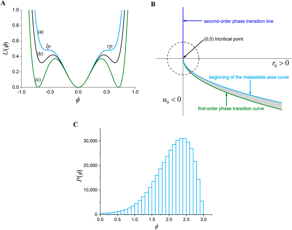
where $\varphi$ denotes the order parameter. The case $\left(r_0,u_0,c_0>0\right)$ corresponds to the symmetrical phase. The case $\left(r_0,c_0>0,u_0<0\right)$ corresponds to the broken symmetry phase, as shown in Figure 2A (Huang, 1987; Contoyiannis et al., 2015). The light blue curve (Figure 2Aa) presents the beginning of a metastable region; when the triple degeneration of the order parameter minima begins to appear in G-L free energy, the black curve (Figure 2Ab) is an intermediate metastable state, whereas the green curve (Figure 2Ac) corresponds to the first-order transition.

Figure 2

Figure 2. (A) G-L free energy $U\left(\varphi \right)$ vs. the order parameter $\varphi$ for the first-order transition of a thermal system of infinite size. (a) Beginning of metastable region, with the two characteristic small plateaus. (b) Intermediate metastable state, where the stable fixed points of the ${\varphi }^6$ theory appear. (c) Completion of the triple degeneration of the order parameter minima signifying the first-order phase transition (Huang, 1987). (B) Phase diagram in the parametric space for the G-L free energy of Equation 5, where the notions of the first-order phase transition, the second-order phase transition, the Griffiths trictitical point, the region “around” it, and the beginning of the metastable area are depicted (see also text). (C) Distribution of the order parameter $\varphi$ values produced by the tricritical intermittent map of Equation 6.

Figure 2B shows a phase diagram in the parametric space for the G-L free energy of Equation 5. The blue line corresponds to the second-order phase transition, the green curve to first-order phase transition curve, and the point at which they meet is known as the “Griffiths tricritical point” (Huang, 1987; Contoyiannis et al., 2015). The dashed-periphery circle symbolizes the notion of “around” (close to) the tricritical point. The beginning of the metastable region is shown by a light blue curve. It is noted that the hatched area between the first-order phase transition curve and the beginning of the metastable region curve denotes the metastable states (e.g., $U\left(\varphi \right)$ of Figure 2Ab). Notably, for part of the “beginning of the metastable area” curve of Figure 2B that falls within the circle, the G-L free energy has the form of Figure 2Aa and, additionally, the two small plateaus (marked as “$lp$” and “$rp$”) are wide enough. It was shown in Contoyiannis et al. (2015) that the existence of these two small (but wide enough) plateaus of Figure 2Aa means that another form of intermittency develops with a fixed point at the value of the order parameter ${\varphi }_0={\varphi }_{lp}$ or ${\varphi }_0={\varphi }_{rp}$.

As demonstrated in Contoyiannis et al. (2015), the fluctuations of the order parameter at this state, simulated by single-spin flip dynamics, are described by the following intermittent map, known as a “tricritical intermittency map”:

${\varphi }_{n+1}={\varphi }_n-u_2{\varphi }_n^{-z_2}+{\epsilon }_n,(6)$

where ${\varphi }_n$ is the $n$th sample of the scaled order parameter, $u_2>0$ is a coupling parameter, $z_2>0$ stands for a characteristic exponent associated with the isothermal exponent $\delta$ as $z_2=\delta +1$, and ${\epsilon }_n$ stands for the non-universal stochastic noise necessary for the creation of ergodicity. Note that, as in Equation 2, in case the exponent is not an integer, the nonlinear term should be used as $-u_2{\left|{\varphi }_n\right|}^{-z_2}$. Note that the 1D map of Equation 6 acts as a repellor that produces the intermittent fluctuations of the order parameter. Specifically, its fixed point is a high value (theoretically infinity) and its non-linear term $-u_2{\varphi }_n^{{-z}_2}$ drives the trajectory away from the laminar region by leading to lower values (Potirakis et al., 2025).

As shown in Contoyiannis et al. (2015), the distribution of laminar lengths $P\left(L\right)$ for the map of Equation 6 is also of the power-law form of Equation 3, whereas for the power-law exponent $p$, the following hold:

$p=\frac{z_2}{z_2+1}=\frac{\delta +1}{\delta +2}.(7)$

Given that the isothermal critical exponent $\delta$ obtains values in the interval $\left(1,+\infty \right)$ (Huang, 1987), it follows that for the map of Equation 6 exponent values $\left.p\in [0.66,1\right)$ are expected. As already mentioned, this new dynamic of the order parameter fluctuations appears only close to the Griffiths tricritical point.

In Figure 2C, we present the distribution of order parameter $\varphi$, when the intermittent map of Equation 6 is run for $4·{10}^5$ iterations, with parameter values $z_2=4,$ $u_2=0.2$ and ${\epsilon }_n\in \left[-0.01,0.01\right]$ (Contoyiannis et al., 2015). This distribution corresponds to the G-L free energy of the form of Figure 2Aa (light blue curve) in the beginning of the metastable area but close to the tricritical point so that the small plateaus are wide enough. It is clear that a high number of the order parameter values are attracted around the G-L free-energy local minimum (fixed point) ${\varphi }_0={\varphi }_{rp}$, where the small (but wide enough) plateau appears.

2.2 Power-law identification in critical and tricritical time series

2.2.1 MCF

The time series analysis method used to find the distribution of laminar lengths (Equation 3) is the method of critical fluctuations (MCF). In the following, we briefly present the key notions of MCF. For a detailed description of the MCF analysis, see Contoyiannis et al. (2002) and Potirakis et al. (2021).

In the application of MCF, two characteristic values of the order parameter amplitude that define the laminar region are used. The first characteristic value is the fixed point ${\varphi }_0$, which in 1D iterative maps like those described by Equations 2 and 6 is determined according to the turning point method (Diakonos and Schmelcher, 1997; Schmelcher and Diakonos, 1997). Note that in symmetrical distributions with a profound plateau, such as the distribution of Figure 1B, the fixed point corresponds to the middle of the plateau; for Figure 1B it is ${\varphi }_0=0$. For other distribution shapes, the fixed point lies on the side of the distribution where the higher probability of occurrence appears, which is the edge of the most “abrupt” side. The second characteristic value is the so-called “end of the laminar region” ${\varphi }_L$ (in positive or negative values due of symmetry), which is a varying parameter.

The laminar lengths $L$ are calculated as the waiting times between the abovementioned two characteristic values—the number of consecutive order parameter values $\varphi$ that, in the case ${\varphi }_0<{\varphi }_L$, satisfy ${\varphi }_0\le \varphi \le {\varphi }_L$. The distribution of laminar lengths $P\left(L\right)$ is calculated and is then checked as to whether it is a power-law; if so, the power-law exponent $p$ of Equation 3 or Equation 6 is estimated.

2.2.2 Wavelet-based detection of scaling behavior in noisy experimental data

To investigate whether the distribution of laminar lengths follows a power-law and to calculate the exponent $p$ of Equation 3 or Equation 6 if a power-law is present, we use a recently introduced method: the wavelet-based detection of scaling behavior in noisy experimental data (Contoyiannis et al., 2020). As explained below, this method has significant advantages in detecting scaling behavior over standard curve-fitting-based methods.

Any function can be expanded on a wavelet basis, while wavelet expansion is suitable for phenomena that exhibit self-similarity, such as critical phenomena, manifested by power-law behavior. In discrete form, the mother wavelet function $\psi \left(x\right)$ undergoes two transformations: change of the scale $j$ and displacement $k$, with $j,k\mathbb{\in }\mathbb{Z}$ producing the wavelet basis elements ${\psi }_{j,k}\left(x\right)=2^{\frac{j}{2}}\psi \left(2^{j}x-k\right)$, with $j=\dots ,-1,0,1,\dots$ and $k=-j,\dots ,-1,0,1,\dots ,j$, whereas the wavelet analysis coefficients are denoted $d_{j,k}$. For $j=k=0$, one gets the coarse-grained description of the analysis. In the framework of this description, the coefficients of the analysis can and do ignore the noise of the signal to be analyzed (Contoyiannis et al., 2020). This behavior has been used to develop an algorithm that applies to any discrete distribution $P\left(i\right),i=1,2,\dots ,N_P$ associated with real or numerical time series. This algorithm can and does answer the question of whether the analyzed distribution embeds a power-law behavior, how close or far is it from the power-law, and what the corresponding power-law exponent $p$ is. In other words, it provides a kind of “fitting” that can be applied to laminar lengths distribution $P\left(L\right)$ without carrying the pathogeny of standard curve-fitting-based methods due to noise in the experimental data. This is especially important at the high values of the laminar lengths, where the poor statistics of the points in the tails of the distributions lead to results of questionable reliability.

In standard curve fitting, only the short scales are usually kept for analysis of the laminar length’ distribution. This is done to avoid the tail of distributions, where the strong noise makes the results vague. However, this is not correct because it brutally removes any information that the long scales may carry. In most cases of calculating the power-law from distributions of laminar lengths (waiting times) $L$ presented in the literature, this is done on long scales ($L\gg 1$) (Schuster and Just, 2005; Alemany and Zanette, 1994; Koponen, 1995; Peng et al., 1992; Stauffer, 1985; Provata, 1999). Thus, long scales carry important information and cannot be excluded from analysis. The Haar wavelet was used to develop the specific algorithm. Its mother function is defined in Equation 8, using the Heaviside step function, $\mathrm{\Theta }\left(z\right)$, as

${\psi }_{\mathrm{{\rm H}}}\left(x\right)=\mathrm{\Theta }\left(\frac{\Delta }{2}-x\right)\mathrm{\Theta }\left(x\right)-\mathrm{\Theta }\left(x-\frac{\Delta }{2}\right)\mathrm{\Theta }\left(\Delta -x\right),(8)$

for $x\in$ ($0,\Delta$], while the wavelet analysis coefficients for the expansion of a power-law function (appropriate for a finite system) $F\left(x\right)=\left\{\begin{array}{ll}0,& x\notin [{\Delta }_{\mathit{min}},{\Delta }_{\mathit{max}})\\ c{x}^{-p},& {\Delta }_{\mathit{min}}\le x<{\Delta }_{\mathit{max}}\end{array}\right.$ can be written as in Equation 9 (Contoyiannis et al., 2020)

$d_{j,k}=c\sqrt{\frac{2^j}{\Delta }}\left({\displaystyle \sum _{i=\mathit{max}\left(\left[k\frac{\Delta }{2^j}\right],1\right)}^{\left[k\frac{\Delta }{2^j}+\frac{\Delta }{2^{j+1}}\right]}}{i}^{-p}-{\displaystyle \sum _{i=\left[k\frac{\Delta }{2^j}+\frac{\Delta }{2^{j+1}}\right]+1}^{\left[\left(k+1\right)\frac{\Delta }{2^j}\right]}}{i}^{-p}\right),(9)$

where $c$ is a normalization constant and $\left[v\right]$ stands for the integer part of a variable $v$.

One can then define the following quantities (Contoyiannis et al., 2020) for the discrete case:

$\lambda =\frac{\frac{d_{00}}{d_{10}}}{\frac{d_{10}}{d_{20}}}=\frac{d_{00}{d}_{20}}{d_{10}^2}=\frac{\left({\displaystyle {\sum }_{i=1}^{\left[\frac{\Delta }{2}\right]}}P\left(i\right)-{\displaystyle {\sum }_{\frac{\Delta }{2}}^{\Delta }}P\left(i\right)\right)\left({\displaystyle {\sum }_{\mathrm{i}=1}^{\left[\frac{\Delta }{8}\right]}}P\left(i\right)-{\displaystyle {\sum }_{\left[\frac{\Delta }{8}\right]}^{\left[\frac{\Delta }{4}\right]}}P\left(i\right)\right)}{{\left({\displaystyle {\sum }_{\mathrm{i}=1}^{\left[\frac{\Delta }{4}\right]}}P\left(i\right)-{\displaystyle {\sum }_{\left[\frac{\Delta }{4}\right]}^{\left[\frac{\Delta }{2}\right]}}P\left(i\right)\right)}^2}(10)$

and

$R=\frac{d_{00}}{d_{10}}=\frac{1}{\sqrt{2}}\frac{\left({\displaystyle {\sum }_{i=1}^{\left[\frac{\Delta }{2}\right]}}P\left(i\right)-{\displaystyle {\sum }_{\frac{\Delta }{2}}^{\Delta }}P\left(i\right)\right)}{\left({\displaystyle {\sum }_{\mathrm{i}=1}^{\left[\frac{\Delta }{4}\right]}}P\left(\mathrm{i}\right)-{\displaystyle {\sum }_{\left[\frac{\Delta }{4}\right]}^{\left[\frac{\Delta }{2}\right]}}P\left(i\right)\right)},(11)$

with $8<\Delta <N_P$.

The specific method has the following steps:

1. We apply Equation 10 to calculate $\lambda$ as a function of $\Delta$ up to a value ${∆}_{\mathit{max}}\le N_P$. We plot $\lambda$ vs. $\Delta$, and since we are interested in the convergence of $\lambda$ (Contoyiannis et al., 2020), we focus on the right-most part of the plot (for large $\Delta$); up to the last ten points ($n={\Delta }_{\mathit{max}}-9,\dots ,{\Delta }_{\mathit{max}}$) (Contoyiannis et al., 2020) are enough to deduce a conclusion. The value of ${∆}_{\mathit{max}}$ is determined in the tail of the distribution of laminar lengths according to the next criterion.

2. We quantify the previous step by calculating the distance of $\lambda$ from the value $\lambda =1$, which denotes an exact power-law, by calculating the quantity:

$Q_{\lambda }=\frac{1}{10}{\sum }_{n={\Delta }_{\mathit{max}}-9}^{{\Delta }_{\mathit{max}}}{\left(1-{\lambda }_n\right)}^2.(12)$

The closer the $Q_{\lambda }$ is to the value 0, the closer to the power-law is the distribution. Therefore, the position of ${∆}_{\mathit{max}}$ is located where the quantity $Q_{\lambda }$ comes closest to zero.

3. We then produce the $R$ vs. $\Delta$ plot using Equation 11. From the convergence region of the plot—that is, for $n={\Delta }_{\mathit{max}}-9,\dots ,{\Delta }_{\mathit{max}}$ (see Equation 12) —mean value $〈R〉$ is obtained for quantity $R$.

4. In place of $P\left(i\right)$, we consider the test function $f\left(i\right)=c_f{i}^{-p},i=1,2,..{∆}_{\mathit{max}}$, where $c_f$ is a constant factor. We then solve Equation 11 numerically for the given $〈R〉$ value with respect to $p$ in order to estimate the value of the $p$ exponent which corresponds to $〈R〉$.

The power-law test function mentioned in Step 4 is used only when $Q_{\lambda }<order\left({10}^{-3}\right)$, which indicates an exact power-law; furthermore, $\left.p\in [1,2\right)$ indicates that the underlying system is in critical state, whereas $\left.p\in [0.66,1\right)$ indicates that the underlying system is close to the tricritical point (Section 2.1). Where $order\left({10}^{-3}\right)<Q_{\lambda }<order\left({10}^{-2}\right)$, this indicates that the examined laminar lengths distribution is close to the power-law. In this case, in Step 4 we can use truncated power-law test function $g\left(i\right)=c_g{i}^{-p}{e}^{-iq},i=1,2,..{∆}_{\mathit{max}}$, where $c_g$ is a constant factor, instead of power-law test function $f\left(i\right)$ to investigate further. Thus, we quantify a power-law with an exponential correction, and if the exponents are found to be $\left.p\in [1,2\right)$ or $\left.p\in [0.66,1\right)$ and $q\approx 0$, the underlying system is in critical state or close to the tricritical point, respectively. In cases that $Q_{\lambda }$ turns out to be higher than $order\left({10}^{-2}\right)$, there is no power-law distribution.

3 Results

3.1 Key notions of the 3D Ising model

A typical example of a finite-size thermal system undergoing second-order phase transition is the well-known Ising spin modeling in three spatial dimensions (or 3D Ising model). In the case of a $Z\left(N\right)$ spin system, spin variables are defined as $s\left(a_i\right)=e^{i2\pi a_i/N}$ (lattice vertices $i=1\dots i_{\mathit{max}}$) with $a_i=0,1,2,3\dots N-1$. The Ising models correspond to the case of $N=2$, where they follow $Z\left(2\right)$ symmetry with two states of spin: $\pm 1$. Moreover, Metropolis et al. (1953) provide an effective algorithm for producing configurations. In this algorithm, the configurations at constant temperatures are selected with Boltzmann statistical weights $e^{-\beta H}$, where $H$ stands for the Hamiltonian of the spin system. The nearest neighbors’ interactions can then be written as in Equation 13:

$H=-{\displaystyle \sum _{<i,j>}}{J}_{ij}{s}_i{s}_j.(13)$

According to this model, a second-order phase transition takes place when the temperature drops below a specific value, the pseudocritical temperature ($T_{pc}$) (Huang, 1987; Kaku, 1993). For lattice length $d=32-$a 32³ 3D Ising model lattice—and for $N_{sim}=2·{10}^6$ , the pseudocritical temperature was found to be $T_{pc}\approx 4.515$ and the SSB completion temperature was found to be $T_{SSB}\approx 4.45$ for ($J_{ij}=1$) (Diakonos et al., 2022). It is noted that both $T_{pc}$ and $T_{SSB}$ depend on the size of the system $d$ and the lattice sweeps $N_{sim}$. Regarding $T_{pc}$, its calculation becomes more accurate by increasing $N_{sim}$.

3.2 Numerical experiment: SSB and beyond for the 3D Ising model

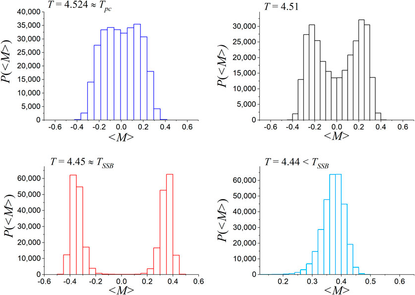
Considering that a sweep of the whole lattice represents the algorithmic time unit and that the possible spin values are $\pm 1$, then by numerically calculating the mean magnetization (order parameter) ${〈M〉}_n$ for each configuration $n$, a trajectory of the fluctuations of mean magnetization $\left\{{〈M〉}_n\right\}$ is produced, which is a time series in algorithmic time. We conducted a numerical experiment by running a 32³ 3D Ising model lattice with $J_{ij}=1$ (Section 3.1) for $N_{sim}=3·{10}^5$ lattice sweeps at different decreasing temperatures: $T=4.524\approx T_{pc}$, $T=4.51$, $T=4.45\approx T_{SSB},$ $T=4.44$, $T=4.4$, $T=4.3$, $T=4.2$, and $T=4$. Indicatively, Figure 3 presents the evolution, sequentially as the temperature drops, of the distribution of these fluctuations from $T_{pc}$ up to just below $T_{SSB}$. The left-top panel of Figure 3 shows the distribution for $T=4.524\approx T_{pc}$. The right-top panel of Figure 3 shows the distribution for an intermediate temperature within the aforementioned hysteresis zone (or SSB-zone) $T=4.51$, where the two lobes communicate with each other. The left-bottom panel of Figure 3 presents the end of the hysteresis zone at the SSB completion temperature $T=4.45\approx T_{SSB}$, where the statistical lobes are ready to separate from each other. The right-bottom panel of Figure 3 illustrates that the two lobes are completely separated at temperature $T=4.44$, just below $T_{SSB}$.

Figure 3

Figure 3. Distributions of the mean magnetization fluctuations of a 32³ lattice of the 3D Ising model for $N_{sim}=3·{10}^5$ lattice sweeps at different decreasing temperatures: $T=4.524\approx T_{pc}$, $T=4.51$, $T=4.45\approx T_{SSB},$ and $T=4.44$, just below $T_{SSB}$.

3.3 Power-law analysis results

As an example of the MCF analysis (Section 2.2.1), we now present the calculation of the laminar lengths $L$ for the time series of the order parameter values ${〈M〉}_n$ of the 3D Ising model of the experiment described in Section 3.2 at $T=4.524\approx T_{pc}$. Especially at this temperature, the distribution of the amplitude values of the mean magnetization time series $\left\{{〈M〉}_n\right\}$ (Figure 3A) is practically symmetrical around the value $〈M〉=0$ (as much as the considered $N_{sim}=3·{10}^5$ lattice sweeps allow) as expected for $T_{pc}$. In order to account for the spin-reversal symmetry of the model but also to increase the accuracy of the power-law exponent estimation by MCF, the absolute value of the mean magnetization $\left\{{\left|〈M〉\right|}_n\right\}$ time series was analyzed instead of $\left\{{〈M〉}_n\right\}$ (Contoyiannis et al., 2002; Contoyiannis and Diakonos, 2007). Therefore, in the application of MCF for this temperature only, the order parameter time series is considered to be the fluctuations of absolute mean magnetization vs. algorithmic time: $\left\{{\varphi }_n\right\}=\left\{{\left|〈M〉\right|}_n\right\}$. The distribution of amplitude values of the $N_{sim}=3·{10}^5$ points-long $\left\{{\left|〈M〉\right|}_n\right\}$ time series analyzed by MCF is shown in Figure 4A. As already mentioned in Section 2.2.1, the laminar lengths $L$ are defined as the waiting times inside the laminar region—the number of consecutive amplitude values of the time series for which ${\varphi }_0\le \varphi \le {\varphi }_L$. Here, the fixed point, ${\varphi }_0$, as determined according to the turning point method (Diakonos and Schmelcher, 1997; Schmelcher and Diakonos, 1997), was found to be ${\varphi }_0=0$. Moreover, the value of ${\varphi }_L$ is varied until at least one ${\varphi }_L$ value for which the distribution $P\left(L\right)$ becomes a power-law is found, if of course there is such a value. Here, it was found that ${\varphi }_L=0.2$. The distribution of laminar lengths inside the laminar region $\left[{\varphi }_0=0,{\varphi }_L=0.2\right]$ is depicted in Figure 4B.

Figure 4

Figure 4. power-law analysis of the 3D Ising model $\left\{{\left|〈M〉\right|}_n\right\}$ time series resulting from the numerical experiment described in Section 3.2 for $T=4.524\approx T_{pc}$. (A) Distribution of $\left|〈M〉\right|$ where the solid vertical line denotes the fixed point ${\varphi }_0=0$ (also known as the start of the laminar regions), whereas the dashed vertical line denotes the end of the laminar region ${\varphi }_L=0.2$. The zone (amplitude values’ interval) delimited between the two horizontal lines is the laminar region. (B) Distribution of laminar lengths (waiting times) inside the laminar region $\left[{\varphi }_0=0,{\varphi }_L=0.2\right]$. (C) Plot of $\lambda$ vs. $\Delta$ (blue dots) for the last ten values of $\Delta$, as computed (Equation 10) for the calculated distribution of laminar lengths. Horizontal black line corresponds to the criterion $\lambda =1$, denoting an exact power-law distribution. (D) Plot of $R$ vs. $\Delta$ (blue dots) for the last ten values of $\Delta$, as computed (Equation 11) for the calculated distribution of laminar lengths shown in right-top panel. Mean value of these ten values is $〈R〉=0.766$ and the power-law exponent was finally estimated to be $\left.p=1.21\in [1,2\right)$, indicating critical dynamics.

We now demonstrate the application of the wavelet-based method for the detection of scaling behavior presented in Section 2.2.2, using as an example the laminar length distribution $P\left(L\right)$ obtained for the 3D Ising model at $T=4.524\approx T_{pc}$ and the laminar region $\left[{\varphi }_0=0,{\varphi }_L=0.2\right]$ (Figure 4B). Although we present here the application for just one ${\varphi }_L$ value (${\varphi }_L=0.2$), it should be noted that the procedure described as follows is repeatedly applied along with the MCF (Section 2.2.1) while the value of ${\varphi }_L$ is varied. Changing the value of ${\varphi }_L$ checks, for each examined ${\varphi }_L$ value, whether the laminar lengths distribution obtained using MCF is a power-law or not. Thus, the ${\varphi }_L$ value leading to a laminar lengths’ distribution closest to power-law (in this case ${\varphi }_L=0.2$) is finally selected. Note that, according to what is presented in Section 2.1, it is expected that the laminar lengths distribution of 3D Ising at the critical state is a power-law with a power-law exponent value $\left.p\in [1,2\right)$, and the underlying dynamics of the fluctuations of the order parameter are that of critical intermittency type I, as described by Equation 2 (Contoyiannis et al., 2002).

The wavelet-based method for the detection of scaling behavior (Section 2.2.2) starts by looking in the tail of the laminar lengths’ distribution for the maximum length ${\Delta }_{\mathit{max}}$ for which the last ten values of $\lambda$ (calculated using Equation 10) lead to the minimum possible value for the quantity $Q_{\lambda }$ (Equation 12). If this value satisfies the criterion $Q_{\lambda }<order\left({10}^{-3}\right)$, then the distribution of laminar lengths is a power-law.

For the distribution of Figure 4B, $Q_{\lambda }=8.9·{10}^{-5}$ for ${\Delta }_{\mathit{max}}=400$. Indeed, the $\lambda$ vs. $\Delta$ plot of the last ten values of $\lambda$ shown in Figure 4C confirms that, for these values of $\Delta$, the calculated $\lambda$ values converge to the value $\lambda =1$, denoting an exact power-law. To find the exponent of the power-law, we calculated the last ten values of the quantity $R$ (using Equation 11) and subsequently calculated their average value $〈R〉=0.766$ (Figure 4D). Then, we numerically solved Equation 11 with respect to $p$ using the test function $f\left(i\right)$ in place of $P\left(i\right)$ (Step 4 of the algorithm) to estimate the value of the $p$ exponent which corresponds to $〈R〉=0.766$. The estimated value is $p=1.21$; since it holds that $\left.p\in [1,2\right)$, this indicates the existence of type I intermittent criticality. Therefore, the 3D Ising system of the experiment of Section 3.1 is indeed in the critical state for $T=4.524\approx T_{pc}$.

We can confirm the correctness of this result through the theory of critical exponents. It is known that the 3D Ising model has an isothermal critical exponent ${\delta }_{3\mathrm{D}-\text{Ising}}=4.8$ (Campostrini et al., 2002). Using Equation 4, the theoretically obtained value for the $p$ exponent at the critical state is $p_{3\mathrm{D}-\text{Ising}/\text{Cr}}=1.21$, which is identical to the value estimated from the numerical data.

As demonstrated by Diakonos et al. (2022), inside the hysteresis zone for temperatures $T_{pc}>T>T_{SSB}$, the distributions of laminar lengths present scaling laws with exponents $\left.p\in [1,2\right)$, whereas by gradually reducing the temperature from $T_{pc}$ to $T_{SSB}$, a gradual transition from type I intermittent dynamics to on–off intermittency (Platt et al., 1993) occurs, with on–off intermittency achieved at $T_{SSB}$. Thus, we could say that this zone is a region of “degeneracy” of the critical point in finite systems. We now examine whether the distribution of laminar lengths is of a power-law form for $T<T_{SSB}$.

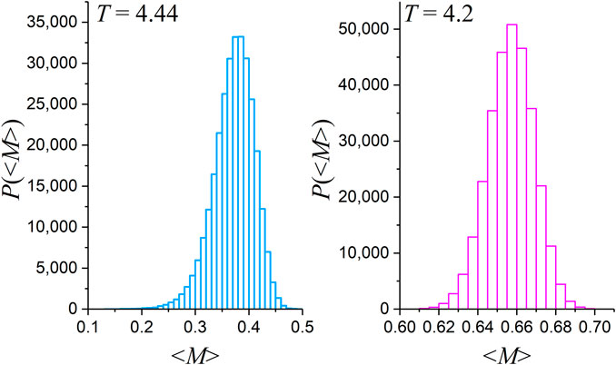
Figure 5 depicts the distributions of the mean magnetization time series $\left\{{〈M〉}_n\right\}$ values resulting from the experiment described in Section 3 for two indicative temperatures $T<T_{SSB}\approx 4.45$: for $T=4.44$, just below $T_{SSB}$ (in an approximation of two decimal places), and an even lower temperature, $T=4.2$. Note that the distribution for $T=4.44$ in Figure 5 is the same as that shown in Figure 3 but with narrower bin size for increased detail. As is evident, for temperatures right after SSB, as in Figure 5 for $T=4.44$, the distribution is not symmetrical but presents a shift of the maximum towards higher values, as well as an extension of its edge towards smaller values. However, as one gets further away from SSB, by further lowering temperature as in Figure 5 for $T=4.2$, the distribution ends up symmetrical again. In all cases beyond the SSB completion temperature, as in Figure 5, the critical point at ${\varphi }_0=0$ ceases to exist as a fixed point in the distributions of the order parameter values. According to the theory of second-order phase transition, beyond the SSB, the critical point has given its position as fixed point to higher values of the order parameter in distributions, as observed in Figure 5. For $T=4.44$, the fixed point, calculated using the turning point method (Diakonos and Schmelcher, 1997; Schmelcher and Diakonos, 1997) (see also Section 2.2.1) was found to be ${\varphi }_0=0.45$. Thus, a displacement of the fixed point from 0 to 0.45 is observed right after the SSB completion.

Figure 5

Figure 5. Distributions of the $\left\{{〈M〉}_n\right\}$ time series values resulting from the numerical experiment described in Section 3.2 at two different decreasing temperatures $T<T_{SSB}\approx 4.45$: right after the SSB, at temperature $T=4.44$, and at an even lower temperature $T=4.2$.

By applying the MCF (Section 2.2.1) to the mean magnetization time series $\left\{{〈M〉}_n\right\}$ corresponding to the values’ distribution for $T=4.44$ (Figure 5), we found that the laminar region is delimited by the abovementioned new fixed point ${\varphi }_0=0.45$ and the end of the laminar region value ${\varphi }_L=0.32$. This value was found by varying the value of ${\varphi }_L$ and applying, for each examined ${\varphi }_L$ value, the wavelet-based method for the detection of scaling behavior to check whether the corresponding laminar lengths’ distribution, obtained using MCF, is a power-law or not (see also Section 2.2.2). The laminar length distribution obtained for $T=4.44$, just below from SSB, for the laminar region $\left[{\varphi }_L=0.32,{\varphi }_0=0.45\right]$ is portrayed in Figure 6.

Figure 6

Figure 6. Laminar lengths distribution inside the laminar region $\left[{\varphi }_L=0.32,{\varphi }_0=0.45\right]$ for the $\left\{{〈M〉}_n\right\}$ time series resulting from the numerical experiment described in Section 3.2 at temperature $T=4.44<T_{SSB}=4.45$.

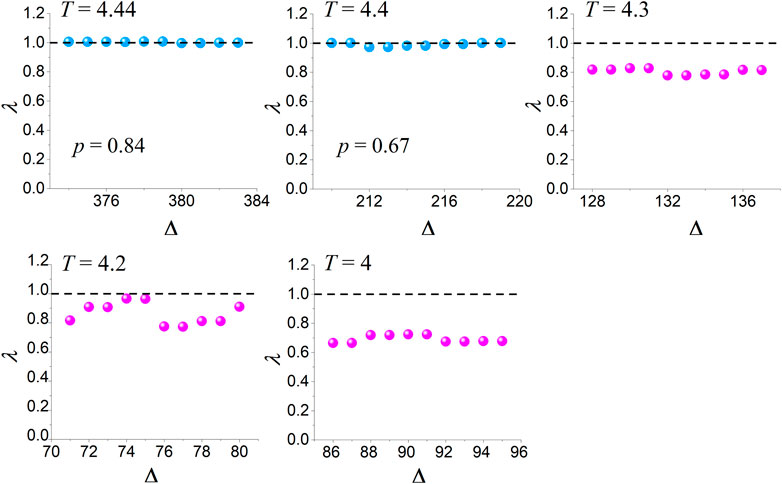
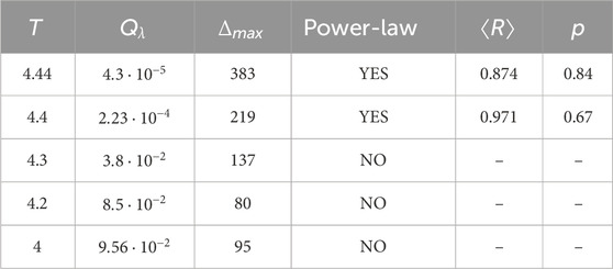
The application of the wavelet-based method for the detection of scaling behavior to the laminar lengths distribution of Figure 6 (see top-left-most graph of Figure 7 and the first row of Table 1) proved that the specific distribution follows a power-law of the form of Equation 3 with exponent value $\left.p=0.84\notin [1,2\right)$, which means that the system, although it presents scaling behavior, is not at the critical state as expected for $T=4.44$—just below $T_{SSB}$. Extending our investigation to even lower temperatures for $T=4.4$, $T=4.3$, $T=4.2$, and $T=4$—all below $T=4.45\approx T_{SSB}$—we summarize the results of the wavelet-based analysis for the detection of scaling behavior in Figure 7 and Table 1. Figure 7 shows the $\lambda$ vs. $\Delta$ plots for the last ten values of $\Delta$ for all the examined temperatures below $T_{SSB}$ (plots similar to Figure 4C). Note that the ${\Delta }_{\mathit{max}}$ parameter for each temperature was determined as explained in Section 2.2.2. As is apparent from Figure 7 and the obtained values of the quantity $Q_{\lambda }$ in Table 1 (see step 2 in Section 2.2.2), $\lambda$ converges to the value $\lambda =1$ ($Q_{\lambda }<order\left({10}^{-3}\right)$), denoting an exact power-law only for $T=4.44$ and $T=4.4$, finally leading to exponent values $p=0.84$ and $p=0.67$, respectively, while for both these estimated exponents $\left.p\notin [1,2\right)$ (no criticality, as expected). For lower temperatures, the obtained values of $\lambda$ do not converge to the value $\lambda =1$, so no power-law is present in the corresponding laminar lengths’ distributions; therefore, at these temperatures the system does not obey scaling laws. The values of all the quantities involved in the wavelet-based analysis for the detection of scaling behavior are summarized in Table 1 for all the temperatures examined below $T_{SSB}$.

Figure 7

Figure 7. Plots of $\lambda$ vs. $\Delta$ for the last ten values of $\Delta$, as computed (Equation 10) for the distributions of laminar lengths obtained (using MCF) for the $\left\{{〈M〉}_n\right\}$ time series resulting from the numerical experiment described in Section 3.2 at different temperatures $T<T_{SSB}=4.45$: $T=4.44$ (laminar lengths’ distribution shown in Figure 6), $T=4.4$, $T=4.3$, $T=4.2$, and $T=4$. Horizontal black line corresponds to the criterion $\lambda =1$, denoting an exact power-law distribution. For temperatures $T=4.44$ and $T=4.4$ the estimated exponent $p$ values are 0.84 and 0.67, respectively. For temperatures below $T=4.4$, no exponent can be estimated since the system has moved away from the power-law behavior.

Table 1

Table 1. Results of wavelet-based analysis for temperatures below the SSB corresponding to Figure 7.

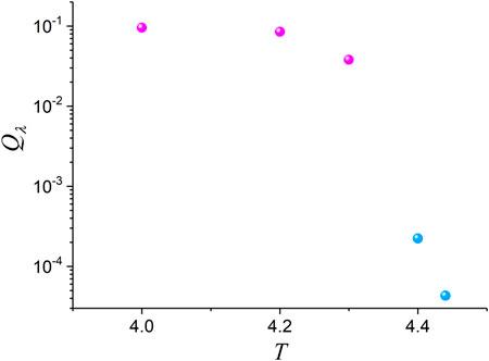
We conclude that there is a narrow temperature zone immediately after the SSB where we find power-laws for the distribution of laminar lengths. Moreover, the obtained power-law exponents have values $p<1$ and, specifically, $\left.p\in [0.66,1\right)$. As already mentioned, the quantity $Q_{\lambda }$ of the applied wavelet-based method for the detection of scaling behavior (Section 2.2.2) is a quantitative criterion expressing the proximity of the relevant dynamics to the power-law. Figure 8 provides a visualization of the obtained $Q_{\lambda }$ of Table 1 vs. $T$ that helps us quantitatively perceive the extent of this narrow post-SSB temperature zone. A sharp transition is observed from the narrow temperature zone immediately after the SSB $4.4\le T<T_{SSB}=4.45$, where we find power-laws for the distribution of laminar lengths (light blue) to even lower temperatures $T<4.4$, where the distribution of laminar lengths strongly deviates from the power-law.

Figure 8

Figure 8. Plot of $Q_{\lambda }$ vs. $T$ for the wavelet-based analysis for temperatures below the SSB corresponding to Table 1.

In second-order phase transition, it is expected that the scaling laws cease to be valid in the phase of broken symmetry; the narrow temperature zone revealed above immediately after the SSB, within which scaling laws are valid for finite-size systems, was unknown until now. Therefore, considering this new information, would it be plausible to argue that within a narrow post-SSB temperature zone, 3D Ising, which is a finite-size system undergoing a second-order phase transition, lingers a bit longer in the critical state owing to its proximity to the SSB? This claim is not correct because, as already mentioned, the power-law exponents obtained $\left.p\notin [1,2\right)$, whereas the existence of criticality holds only for $\left.p\in [1,2\right)$ (Section 2.1). Consequently, we arrive at the conclusion that a different type of dynamics (other than critical dynamics) governs the order parameter fluctuations in this narrow post-SSB zone. The question arising is what kind of dynamics is this and how its emergence can be interpreted. The answer to this question is the subject of Section 4.

4 Discussion

Attempting to answer the question of which dynamics govern the narrow post-SSB temperature zone revealed in Section 3.3 and how its emergence can be interpreted, we initially draw the attention of the reader to the distribution of the mean magnetization time series $\left\{{〈M〉}_n\right\}$ values for $T=4.44<T_{SSB}\approx 4.45$, just below $T_{SSB}$ (Figure 5). We observe that this distribution presents a similarity to the distribution of Figure 2C, which is the distribution of the order parameter $\varphi$ values produced by the tricritical intermittent map of Equation 6. Specifically, it is apparent that they share two common characteristic features: (a) they both present an asymmetry with respect to their peak—an extension of the tail at small values to almost zero is present in both; (b) the peak has been shifted to higher values than the peak at zero for the unbroken symmetry case.

As a consequence of the above observation, one may claim that within the revealed narrow temperature zone right after SSB, the dynamics of the order parameter fluctuations of 3D Ising are no longer governed by the critical intermittency that the map of Equation 2 presents (see Section 2.1). Instead, the order parameter fluctuations in the narrow post-SSB zone are governed by the intermittency dynamics expressed by the map of Equation 6, which are the dynamics appearing around (close to) the tricritical point (see Section 2.1).

Equation 7 (Section 2.1) provides relations that connect the characteristic exponent $z_2$ of the tricritical map of Equation 6 and the isothermal exponent $\delta$ with the power-law exponent $p$ for the distribution of laminar lengths. The above claim could be confirmed by setting ${\delta }_{3\mathrm{D}-\text{Ising}}=4.8$, which, as already mentioned, is the value of the isotherm critical exponent of the universality class of the 3D Ising model (Campostrini et al., 2002) in Equation 7. This results in a theoretically expected power-law exponent $p$ value, $p_{3\mathrm{D}-\text{Ising}/\text{tricr}.}=0.85$. The specific value is very close to that obtained in Section 3.3 for the 3D Ising model at $T=4.44$, which is $p=0.84$ (Table 1), supporting the claim that the 3D Ising model studied is governed by tricritical intermittency dynamics at the specific temperature.

The tricritical intermittent map of Equation 6 has been presented in Section 2.1 within the framework of a thermal system undergoing first-order phase transition (${\varphi }^6$ theory for infinite-size systems). However, as already mentioned, it describes the dynamics only for part of the beginning of the metastable area curve of Figure 2B that is located around (close to) the tricritical point—thus expressing tricritical dynamics. In terms of G-L free energy, this corresponds to the two small (but wide enough) plateaus of the curve (a) (light blue curve) of Figure 2A. The 3D Ising is a finite-size system exhibiting a second-order phase transition which, for infinite-size systems, is described by ${\varphi }^4$ theory. Note that in ${\varphi }^4$ theory, the aforementioned two small plateaus in the G-L free energy around a sole vacuum at $\varphi =0$ are not provided since for any $T<T_c$ the vacuum at $\varphi =0$ vanishes. However, as shown in Figure 2A, the tricritical point can be approached both from the second- and first-order transition. Therefore, one could argue that our results imply that the tricritical intermittent map of Equation 6 expresses the order parameter fluctuation dynamics close to the tricritical point regardless of the path from which the tricritical point is approached in the phase diagram (Figure 2B).

We consider that this was possible to observe due to the finite-size of 3D Ising, as happened with the hysteresis zone, $T_{SSB}<T<T_{pc}$, within which the SSB is gradually completing, although also not predicted by ${\varphi }^4$ theory. It is clarified that the revealed tricritical dynamics in 3D Ising by no means imply that 3D Ising is compatible with ${\varphi }^6$ theory. However, due to its finite size in a very narrow temperature zone just below $T_{SSB}$, the system presents the aforementioned asymmetrical distribution of the mean magnetization time series values that present an extension of the tail at small values to almost zero, as happens for part of the beginning of metastable area close to the tricritical point in ${\varphi }^6$ theory (where this asymmetry is due to the presence of the vacuum at $\varphi =0$ as the sole vacuum).

In summary, we suggest the following possible explanation for the post-SSB behavior that was revealed by our results. By lowering the temperature to just below $T_{SSB}$ and only within a very narrow post-SSB temperature zone, the 3D Ising model and probably any finite-size system undergoing second-order transition approaches the tricritical point from the second-order phase transition line (Figure 2B). Within the specific temperature zone, its order parameter fluctuations are governed by tricritical dynamics, expressed by the tricritical intermittent map of Equation 6.

Overall, the following picture is apparent for the 3D Ising model in terms of the power-law behavior of the laminar lengths’ distribution and the dynamics of the fluctuations of the order parameter. Due to the finite-size nature of 3D-Ising, consecutively as temperature decreases from $T_{pc}$ to beyond $T_{SSB}$:

(a) at $T=T_{pc}$, the laminar lengths’ distribution is a power-law with exponent compatible with critical dynamics $\left.p\in [1,2\right)$, and these dynamics are of type I intermittency (Contoyiannis and Diakonos, 2000; Contoyiannis et al., 2002);

(b) power-law exponents compatible with critical dynamics $\left.p\in [1,2\right)$ are present, and a gradual transition from type I intermittent dynamics to on–off intermittency occurs within the hysteresis zone $T_{SSB}<T<T_{pc}$ as $T$ decreases from $T_{pc}$ to $T_{SSB}$ (Diakonos et al., 2022) (see also Sections 1 and 3.3);

(c) at $T=T_{SSB}$, the laminar lengths’ distribution is a power-law with exponents compatible with critical dynamics $\left.p\in [1,2\right)$, and these dynamics are of on–off intermittency (Diakonos et al., 2022);

(d) as shown in Section 3.3 (Table 1) and discussed above, within a narrow post-SSB temperature zone, the laminar lengths’ distribution is a power-law exponent compatible with tricritical dynamics $\left.p\in [0.66,1\right)$. For the 3D Ising system of the experiment in Section 3.1, this zone is delimited as $4.4\le T<T_{SSB}\approx 4.45$. Analogous to what happens for the hysteresis zone $T_{SSB}<T<T_{pc}$, the width of the very narrow temperature zone just below $T_{SSB}-$within which traces of tricritical dynamics are detected in a finite-size thermal system presenting a second-order phase transition—is expected the increase as the size of the system decreases.

Moreover, as demonstrated in (Diakonos et al., 2022), the autocorrelation function of the order parameter presents an anomalous enhancement at $T=T_{SSB}$. Figure 9 presents the normalized autocorrelation function $C\left(m\right)/C\left(0\right)$ of the mean magnetization time series $\left\{{〈M〉}_n\right\}$ resulting from the experiment in Section 3.1 for $T=4.524\approx T_{pc}$, $T=4.45\approx T_{SSB}$, $T=4.44$, and $T=4.3$. Note that Figure 9 focuses on the first 200 lag steps to highlight the different behaviors for the different temperatures. From Figure 9, one can easily identify the maximization of the time series memory at $T=4.45\approx T_{SSB}$. On the other extreme, the sharp drop (rapid decay) of $C\left(m\right)/C\left(0\right)$ at $T=4.3$ practically indicates absence of memory. This recalls that $T=4.3$ is the only temperature presented in Figure 9 for which the laminar lengths’ distribution is not a power-law. At the pseudocritical temperature, the system presents slow decay of the autocorrelation, which indicates extended memory, as expected for the critical state. At $T=4.44$, just below $T_{SSB}$, the autocorrelation function also presents slow decay; however, it presents memory not as long as in the critical state. In general, the presence of a power-law distribution in laminar lengths (waiting times) of a dynamical system indicates that the system lacks a characteristic or privileged timescale—a hallmark of scale-free behavior. This scale invariance leads to the emergence of long-range temporal correlations, as reflected in the slow decay of the autocorrelation function—a signature of memory effects.

Figure 9

Figure 9. Normalized autocorrelation function $C\left(m\right)/C\left(0\right)$ for the mean magnetization time series $\left\{{〈M〉}_n\right\}$ resulting from experiment in Section 3.1 as temperature decreases from $T_{pc}$ to beyond $T_{SSB}$.

For an infinite-size system undergoing a second-order transition, no power-law behavior and no memory is expected as soon as the symmetry is broken for $T=T_c^{-}$, just below $T_c$. However, in a finite-size system such as the 3D Ising model, not only is the memory and power-law behavior preserved up to $T=T_{SSB}<T_{pc}$, but the anomalous enhancement of autocorrelation at $T=T_{SSB}$, which expresses a maximization of the system’s memory, also seems to permit the finite-size system to retain some memory for even lower temperatures within a narrow post-SSB temperature zone. Within this zone, the system still presents power-law behavior, but the dynamics cannot any longer be critical dynamics since the vacuum at $\varphi =0$ has disappeared at $T=T_{SSB}$. Building upon the retained memory, the fluctuations of the order parameter develop intermittent dynamics for this temperature zone, although around another fixed point ${\varphi }_0>0$. Within this narrow post-SSB temperature zone, the power-law exponent of laminar lengths distribution and the asymmetry of the order parameter distributions indicate tricritical intermittency dynamics, so the finite-size nature of the system may permit its approach close to the tricritical point, although the system does not exhibit first-order phase transition.

5 Conclusion

This study detected power-laws beyond SSB for 3D Ising model, in contrast to what is expected for infinite systems undergoing second-order phase transition. The results obtained show that these power-laws are not compatible with type I critical intermittency dynamics; this was expected since SSB has been completed. Specifically, within a very narrow temperature zone just below the SSB completion temperature $T_{SSB}$ <$T_{pc}$ at which SSB is achieved, 3D Ising’s order parameter fluctuations were shown to be compatible with tricritical intermittency dynamics. This result is in agreement with the consistent appearance of indications of power-laws compatible with tricritical dynamics after SSB in the analysis of MHz FEME time series, which was the motive for this study.

This behavior, which is not predicted by ${\varphi }^4$ theory that describes infinite-size systems undergoing second-order phase transitions, could be observed due to the finite-size nature of the 3D Ising model. Based on the fact that the region where second-order and first-order transitions meet is around the Griffiths tricritical point, a plausible interpretation of our finding is that the 3D Ising model, and probably any finite-size system undergoing second-order transition, approaches the tricritical point from the second-order phase transition line within the very narrow temperature zone revealed, just below the SSB completion temperature.

Future research could check whether the behavior observed for 3D Ising is also observed in other finite-size numerical or real systems exhibiting second-order phase transition.

Data availability statement

The raw data supporting the conclusions of this article will be made available by the authors, without undue reservation.

Author contributions

YC: conceptualization, data curation, formal analysis, investigation, methodology, software, writing – original draft. SP: conceptualization, data curation, formal analysis, investigation, methodology, software, validation, visualization, writing – original draft. SS: conceptualization, validation, visualization, writing – review and editing. MH: validation, visualization, writing – review and editing. PP: visualization, writing – review and editing. N-LM: visualization, writing – review and editing.

Funding

The author(s) declare that no financial support was received for the research and/or publication of this article.

Conflict of interest

The authors declare that the research was conducted in the absence of any commercial or financial relationships that could be construed as a potential conflict of interest.

The author(s) declared that they were an editorial board member of Frontiers at the time of submission. This had no impact on the peer review process or the final decision.

Generative AI statement

The author(s) declare that no Generative AI was used in the creation of this manuscript.

Publisher’s note

All claims expressed in this article are solely those of the authors and do not necessarily represent those of their affiliated organizations, or those of the publisher, the editors and the reviewers. Any product that may be evaluated in this article, or claim that may be made by its manufacturer, is not guaranteed or endorsed by the publisher.

References

Alemany, P., and Zanette, D. (1994). Fractal random walks from a variational formalism for Tsallis entropies. Phys. Rev. E 49, R956–R958. doi:10.1103/PhysRevE.49.R956

PubMed Abstract | CrossRef Full Text | Google Scholar

Andersen, J. V., Sornette, D., and Leung, K.-T. (1997). Tricritical behavior in rupture induced by disorder. Phys.Rev. Lett. 78, 2140–2143. doi:10.1103/PhysRevLett.78.2140

CrossRef Full Text | Google Scholar

Anderson, P. W. (1972). More is different. Science 177 (4047), 393–396. doi:10.1126/science.177.4047.393

PubMed Abstract | CrossRef Full Text | Google Scholar

Barber, M. N. (1983). “Finite-size scaling,” in Phase transitions and critical phenomena. Editors C. Domb, and J. L. Lebowitz (London: Academic Press).

Google Scholar

Beekman, A. J., Rademaker, L., and van Wezel, J. (2019). An introduction to spontaneous symmetry breaking. SciPost Phys. Lect. Notes 11, 11–140. doi:10.21468/SciPostPhysLectNotes.11

CrossRef Full Text | Google Scholar

Binder, K. (1992). Finite size effects at phase transitions. Lect. Notes Phys. 409, 59–125. doi:10.1007/3-540-55997-3_31

CrossRef Full Text | Google Scholar

Brankov, J. G., Dantchev, D. M., and Tonchev, N. S. (2000). Theory of critical phenomena in finite-size systems: scaling and quantum effects. Singapore: World Scientific.

Google Scholar

Brézin, E. (2010). Introduction to statistical field theory. Cambridge, UK: Cambridge University Press. doi:10.1017/CBO9780511761546

CrossRef Full Text | Google Scholar

Brézin, E., and Zinn-Justin, J. (1985). Finite size effects in phase transitions. Nucl. Phys. B 257, 867–893. doi:10.1016/0550-3213(85)90379-7

CrossRef Full Text | Google Scholar

Campostrini, M., Pelissetto, A., Rossi, P., and Vicari, E. (2002). 25th-order high-temperature expansion results for three-dimensional Ising-like systems on the simple-cubic lattice. Phys. Rev. E 65, 066127. doi:10.1103/PhysRevE.65.066127

PubMed Abstract | CrossRef Full Text | Google Scholar

Contoyiannis, Y., and Diakonos, F. (2000). Criticality and intermittency in the order parameter space. Phys. Lett. A 268, 286–292. doi:10.1016/S0375-9601(00)00180-8

CrossRef Full Text | Google Scholar

Contoyiannis, Y., Hanias, M. P., Papadopoulos, P., Stavrinides, S. G., Kampitakis, M., Potirakis, S. M., et al. (2021). Tachyons and solitons in spontaneous symmetry breaking in the frame of field theory. Symmetry 13 (8), 1358. doi:10.3390/sym13081358

CrossRef Full Text | Google Scholar

Contoyiannis, Y., and Potirakis, S. M. (2018). Signatures of the symmetry breaking phenomenon in pre-seismic electromagnetic emissions. J. Stat. Mech. 2018, 083208. doi:10.1088/1742-5468/aad6ba

CrossRef Full Text | Google Scholar

Contoyiannis, Y., Potirakis, S. M., Eftaxias, K., and Contoyianni, L. (2015). Tricritical crossover in earthquake preparation by analyzing pre-seismic electromagnetic emissions. J. Geodyn. 84, 40–54. doi:10.1016/j.jog.2014.09.015

CrossRef Full Text | Google Scholar

Contoyiannis, Y., Potirakis, S. M., Kopanas, J., Antonopoulos, G., Eftaxias, K., and Nomicos, C. (2025). On the recent seismic activity at Ioannina (Greece): pre-earthquake electromagnetic emissions with critical and tricritical behavior. arXiv 0809. Available online at: http://arxiv.org/abs/1610.06220. (Accessed: 10 April 2025).

Google Scholar

Contoyiannis, Y. F., and Diakonos, F. K. (2007). Unimodal maps and order parameter fluctuations in the critical region. Phys. Rev. E 76, 031138. doi:10.1103/PhysRevE.76.031138

PubMed Abstract | CrossRef Full Text | Google Scholar

Contoyiannis, Y. F., Diakonos, F. K., and Malakis, A. (2002). Intermittent dynamics of critical fluctuations. Phys. Rev. Lett. 89 (3), 035701. doi:10.1103/PhysRevLett.89.035701

PubMed Abstract | CrossRef Full Text | Google Scholar

Contoyiannis, Y. F., Potirakis, S. M., and Diakonos, F. K. (2020). Wavelet-based detection of scaling behavior in noisy experimental data. Phys. Rev. E 101 (5), 052104. doi:10.1103/PhysRevE.101.052104

PubMed Abstract | CrossRef Full Text | Google Scholar

Diakonos, F. K., Contoyiannis, Y. F., and Potirakis, S. M. (2022). Subcritical jump probability and anomalous order parameter autocorrelations. EPL 140, 11002. doi:10.1209/0295-5075/ac9158

CrossRef Full Text | Google Scholar

Diakonos, F. K., and Schmelcher, P. (1997). Turning point properties as a method for the characterization of the ergodic dynamics of one-dimensional iterative maps. Chaos An Interdiscip. J. Nonlinear Sci. 7 (2), 239–244. doi:10.1063/1.166249

PubMed Abstract | CrossRef Full Text | Google Scholar

Fisher, M. E. (1998). Renormalization group theory: its basis and formulation in statistical physics. Rev. Mod. Phys. 70 (2), 653–681. doi:10.1103/RevModPhys.70.653

CrossRef Full Text | Google Scholar

Fisher, M. E., and Barber, M. N. (1972). Scaling theory for finite-size effects in the critical region. Phys. Rev. Lett. 28 (23), 1516–1519. doi:10.1103/PhysRevLett.28.1516

CrossRef Full Text | Google Scholar

Folk, R., and Moser, G. (2006). Critical dynamics: a field-theoretical approach. J. Phys. A Math. Gen. 39, R207–R313. doi:10.1088/0305-4470/39/24/R01

CrossRef Full Text | Google Scholar

Fytas, N. G., Martín-Mayor, V., Parisi, G., Picco, M., and Sourlas, N. (2023). Finite-size scaling of the random-field Ising model above the upper critical dimension. Phys. Rev. E 108, 044146. doi:10.1103/PhysRevE.108.044146

PubMed Abstract | CrossRef Full Text | Google Scholar

Goldenfeld, N. (1992). Lectures on phase transitions and the renormalization group. 1st ed. Boca Raton, FL: CRC Press. doi:10.1201/9780429493492

CrossRef Full Text | Google Scholar

Griffiths, R. B. (1970). Thermodynamics near the two-fluid critical mixing point in He³-He⁴. Phys. Rev. Lett. 24, 715–717. doi:10.1103/PhysRevLett.24.715

CrossRef Full Text | Google Scholar

Hasenbusch, M. (2010). Finite size scaling study of lattice models in the three-dimensional Ising universality class. Phys. Rev. B 82 (17), 174433. doi:10.1103/PhysRevB.82.174433

CrossRef Full Text | Google Scholar

Hasenbusch, M., Pelissetto, A., and Vicari, E. (2008). The critical behavior of 3D Ising spin glass models: universality and scaling corrections. J. Stat. Mech. 2008, L02001. doi:10.1088/1742-5468/2008/02/L02001

CrossRef Full Text | Google Scholar

Huang, K. (1987). Statistical mechanics. 2nd Ed. New York: Wiley.

Google Scholar

Kaku, M. (1993). Quantum field theory: a modern introduction. New York: Oxford University Press.

Google Scholar

Koponen, I. (1995). Analytic approach to the problem of convergence of truncated Levy flights towards the Gaussian stochastic process. Phys. Rev. E 52, 1197–1199. doi:10.1103/PhysRevE.52.1197

PubMed Abstract | CrossRef Full Text | Google Scholar

Landau, L. D., and Lifshitz, E. M. (2013). Statistical physics. 3rd ed. Oxford, UK: Elsevier.

Google Scholar

Liu, Z., Vatansever, E., Barkema, G. T., and Fytas, N. G. (2023). Critical dynamical behavior of the Ising model. Phys. Rev. E 108 (3), 034118. doi:10.1103/PhysRevE.108.034118

PubMed Abstract | CrossRef Full Text | Google Scholar

Metropolis, N., Rosenbluth, A. W., Rosenbluth, M. N., Teller, A. H., and Teller, E. (1953). Equation of state calculations by fast computing machines. J. Chem. Phys. 21, 1087–1092. doi:10.1063/1.1699114

CrossRef Full Text | Google Scholar

Minganti, F., Arkhipov, I. I., Miranowicz, A., and Nori, F. (2021). Continuous dissipative phase transitions with or without symmetry breaking. New J. Phys. 23 (12), 122001. doi:10.1088/1367-2630/ac3db8

CrossRef Full Text | Google Scholar

Pathria, R. K., and Beale, P. D. (2022). Statistical mechanics. 4th ed. London: Academic Press. doi:10.1016/B978-0-08-102692-2.00021-1

CrossRef Full Text | Google Scholar

Pelissetto, A., and Vicari, E. (2002). Critical phenomena and renormalization-group theory. Phys. Rep. 368 (6), 549–727. doi:10.1016/S0370-1573(02)00219-3

CrossRef Full Text | Google Scholar

Peng, C.-K., Buldyrev, S. V., Goldberger, A. L., Havlin, S., Sciortino, F., Simons, M., et al. (1992). Long-range correlations in nucleotide sequences. Nature 356, 168–170. doi:10.1038/356168a0

PubMed Abstract | CrossRef Full Text | Google Scholar

Platt, N., Spiegel, E. A., and Tresser, C. (1993). On-off intermittency: a mechanism for bursting. Phys. Rev. Lett. 70, 279–282. doi:10.1103/PhysRevLett.70.279

PubMed Abstract | CrossRef Full Text | Google Scholar

Potirakis, S. M., Contoyiannis, Y., Schekotov, A., Eftaxias, K., and Hayakawa, M. (2021). Evidence of critical dynamics in various electromagnetic precursors. Eur. Phys. J. Spec. Top. 230, 151–177. doi:10.1140/epjst/e2020-000249-x

CrossRef Full Text | Google Scholar

Potirakis, S. M., Diakonos, F. K., and Contoyiannis, Y. F. (2025). A spike train production mechanism based on intermittency dynamics. Entropy 27 (3), 267. doi:10.3390/e27030267

PubMed Abstract | CrossRef Full Text | Google Scholar

Potirakis, S. M., Papadopoulos, P., Matiadou, N. L., Hanias, M. P., Stavrinides, S. G., Balasis, G., et al. (2023). Spontaneous symmetry breaking in systems obeying the dynamics of on–off intermittency and presenting bimodal amplitude distributions. Symmetry 15 (7), 1448. doi:10.3390/sym15071448

CrossRef Full Text | Google Scholar

Provata, A. (1999). Random aggregation models for the formation and evolution of coding and non-coding DNA. Phys. A Stat. Mech. its Appl. 264, 570–580. doi:10.1016/S0378-4371(98)00546-9

CrossRef Full Text | Google Scholar

Quintana, M., and Berger, A. (2023). Experimental observation of critical scaling in magnetic dynamic phase transitions. Phys. Rev. Lett. 131 (11), 116701. doi:10.1103/PhysRevLett.131.116701

PubMed Abstract | CrossRef Full Text | Google Scholar

Ryder, L. H. (1985). Quantum field theory. Cambridge: Cambridge University Press.

Google Scholar

Sakhi, S. (2021). Renormalization functions of the tricritical O(N)-symmetric Φ⁶ model beyond the next-to-leading order in 1/N. J. Phys. Commun. 5, 055011. doi:10.1088/2399-6528/abfe4b

CrossRef Full Text | Google Scholar

San Miguel, M. (2023). Frontiers in complex systems. Front. Complex Syst. 1, 1080801. doi:10.3389/fcpxs.2023.1080801

CrossRef Full Text | Google Scholar

Schmelcher, P., and Diakonos, F. K. (1997). A turning point analysis of the ergodic dynamics of iterative maps. Int. J. Bifurc. Chaos 07, 2459–2474. doi:10.1142/S0218127497001643

CrossRef Full Text | Google Scholar

Schuster, H. G., and Just, W. (2005). Deterministic chaos: an introduction. 2nd Ed. Weinheim: Wiley-VCH Verlag GmbH and Co.

Google Scholar

Solé, R. V., Manrubia Cuevas, S., Luque, B., Delgado, J., and Bascompte, J. (1996). Phase transitions and complex systems: simple, nonlinear models capture complex systems at the edge of chaos. Complexity 1, 13–23. doi:10.1002/cplx.6130010405

CrossRef Full Text | Google Scholar

Sornette, D., and Andersen, J. V. (1998). Scaling with respect to disorder in time-to-failure. Eur. Phys. J. B 1, 353–357. doi:10.1007/s100510050194

CrossRef Full Text | Google Scholar

Stanley, H. E. (1971). Introduction to phase transitions and critical phenomena. Oxford, UK: Oxford University Press.

Google Scholar

Stanley, H. E. (1999). Scaling, universality, and renormalization: three pillars of modern critical phenomena. Rev. Mod. Phys. 71 (2), 358–366. doi:10.1103/RevModPhys.71.S358

CrossRef Full Text | Google Scholar

Stauffer, D. (1985). Introduction to probability theory and its applications. New York: Willey.

Google Scholar

West, G. (2017). “Scale. The universal laws of growth, innovation, sustainability, and the pace of life in organisms, cities,” in Economies and companies. London: Penguin Press.

Google Scholar

Wong, C.-Y. (1994). Introduction to high-energy heavy-ion collisions. Singapore: World Scientific.

Google Scholar