M-PSGP: a momentum-based proximal scaled gradient projection algorithm for nonsmooth optimization with application to image deblurring

In this study, we focus on investigating a nonsmooth convex optimization problem involving the l₁-norm under a non-negative constraint, with the goal of developing an inverse-problem solver for image deblurring. Research focused on solving this problem has garnered extensive attention and has had a significant impact on the field of image processing. However, existing optimization algorithms often suffer from overfitting and slow convergence, particularly when working with ill-conditioned data or noise. To address these challenges, we propose a momentum-based proximal scaled gradient projection (M-PSGP) algorithm. The M-PSGP algorithm, which is based on the proximal operator and scaled gradient projection (SGP) algorithm, integrates an improved Barzilai-Borwein-like step-size selection rule and a unified momentum acceleration framework to achieve a balance between performance optimization and convergence rate. Numerical experiments demonstrate the superiority of the M-PSGP algorithm over several seminal algorithms in image deblurring tasks, highlighting the significance of our improved step-size strategy and momentum-acceleration framework in enhancing convergence properties.

1 Introduction

In the field of image deblurring, the solution of inverse problems can usually be attributed to the solution of constrained optimization problems; thus, the development of optimization solvers for inverse problems with constraints has been a subject of intense research interest. Significantly, the constrained optimization problems arising from image restoration tasks, i.e., denoising, inpainting, and deblurring, can be defined as follows (Bonettini et al., 2008):

$\begin{array}{ll}minf(x),\text{\hspace{1em}s.t.\hspace{1em}}x\in {S},& (1)\end{array}$

where f(x) is a convex function measuring the divergence between the restored and measured data. Due to the ill-posedness of the image restoration problem, a composite regularized function, given by the sum of a fit-to-data function and a penalty function, can be considered to achieve a trade-off between data fidelity and iteration convergence (Tang et al., 2023). Due to the sparsity of image issues, the penalty term generally uses a nonsmooth function, i.e., the l₁-norm; then, the regularized optimization problem can be formed as (Malitsky and Mishchenko, 2024):

$\begin{array}{ll}minf(x)+g(x),\text{\hspace{1em}s.t.\hspace{1em}}x\in {S},& (2)\end{array}$

where f(x) is the discrepancy term, which could be smooth, and g(x) is the nonsmooth penalty term. To address this regularized and nonsmooth optimization problem, the proximal gradient method (PGM) is regarded as a robust and efficient approach. PGM is particularly effective in large-scale and high-dimensional composite optimization problems, with wide applications in signal processing (Wang, 2025) and image restoration (Liu et al., 2019). To address the composite optimization problem (Equation 2), the PGM combines gradient descent with a proximal operator on the penalty term, as shown as follows (Parikh and Boyd, 2014):

$\begin{array}{l}\begin{array}{c}{y}_k={\text{prox}}_{{\alpha }_{k}g}(x_k-{\alpha }_k\nabla f(x_k)),\end{array}\end{array}$

where α_k > 0 is the step size for gradient descent, and the proximal operator for the penalty function g is defined as follows:

$\begin{array}{l}\begin{array}{c}{\text{prox}}_{{\alpha }_{k}g}(x)=\underset{z\in {ℝ}^N}{argmin}{\alpha }_{k}g(z)+\frac{1}{2}\left|\right|x-z|{|}^2.\end{array}\end{array}$

By invoking the proximal operator, the PGM effectively manages non-smooth components and promotes sparse solutions, thus outperforming traditional gradient-based techniques in non-smooth optimization contexts (Aravkin et al., 2022). Classically, the two-step iterative shrinkage thresholding (TwIST) algorithm extends the PGM by introducing a momentum term that relies on the two previous iterations, leading to faster convergence rates for ill-conditioned problems (Bioucas-Dias and Figueiredo, 2007). Thereafter, the fast iterative shrinkage thresholding (FISTA) algorithm was proposed, which improves the PGM by incorporating the Nesterov momentum term and an adaptive step size, thereby accelerating the global convergence rate (Beck and Teboulle, 2009). Moreover, optimization problems in practical applications are often constrained by domain-specific requirements, which motivate the development of the gradient projection method (GPM) to address constrained optimization problems (Zhou et al., 2025). For solving Equation 1, the GPM combines gradient descent with a projection operator, leading to the following iteration:

$\begin{array}{l}{y}_k={\Pi }_{{S}}(x_k-{\alpha }_k\nabla f(x_k)),\end{array}$

in which the projection operator of a vector x ∈ ℝ^N onto the region set $\mathcal{S}$ is defined as follows:

$\begin{array}{l}\begin{array}{c}{\Pi }_{{S}}(x)=\underset{z\in {S}}{argmin}\frac{1}{2}\left|\right|x-z|{|}^2.\end{array}\end{array}$

The projection operation can achieve minimal computational expense while restricting the iterative vector onto the feasible set $\mathcal{S}$. This is evident in the specific case of problem (Equation 2), i.e., lasso regression and ridge regression, where projection can be computed in linear time (Maroni et al., 2025). Consequently, the GPM and its improvements stand as credible schemes to address image deblurring tasks, thanks to their low per-iteration computational overhead (Chen et al., 2025).

Through an optimized fusion of PGM and GPM, a scaled gradient projection (SGP) algorithm was proposed to address the constrained composite problem (Equation 2) (Bonettini and Prato, 2015). The SGP algorithm introduces a scaling matrix D_k during the proximal gradient descent; that is,

$\begin{array}{ll}{y}_k={\Pi }_{{S},D_k}\left[{\text{prox}}_{{\alpha }_{k}g}^{D_k^{-1}}(x_k-{\alpha }_k{D}_k\nabla f(x_k))\right].& (3)\end{array}$

Compared with the FISTA algorithm, SGP demonstrates superior convergence rates and enhances deblurring performance. Recently, aiming to accelerate the solution of the composite optimization method, an optimal accelerated composite optimization (OptISTA) algorithm to solve Equation 2 was developed, which improves FISTA by optimizing the step size via a double-function method and theoretically establishes an exact matching lower bound for composite optimization problems (Jang et al., 2025). Afterwards, the improved OptISTA (IOptISTA) algorithm was proposed, which incorporates a weighting matrix technique and achieves superior numerical performance in image deblurring tasks (Wang et al., 2025).

To accelerate convergence during optimization, the Barzilai-Borwein rules, which serve as adaptive step-size strategies that determine step sizes without relying on online searches, have been widely investigated and improved (He et al., 2023). Serving as an effective and seminal step-size selection strategy, the Barzilai-Borwein (BB) step-size selection rules have garnered significant attention, which approximate the Hessian matrix inverse in a quasi-Newton manner, providing a step size that can adaptively adjust to the descent direction of the problem, which leads to faster convergence rates (Barzilai and Borwein, 1988). Recently, in the context of l₁-regularized problems, a novel step-size selection rule within the proximal gradient framework was proposed, which achieves acceleration by preemptively identifying the optimal redundant components using the spectral properties of the BB step size (Crisci et al., 2024). Beyond step-size improvement, momentum methods provide additional convergence acceleration (Zhang et al., 2023). Classically, the Heavy-Ball (HB) algorithm leverages momentum from past gradients to amplify descent directions, thereby improving convergence rates in ill-conditioned optimization landscapes (Polyak, 1964). Afterwards, Nesterov proposed an Accelerated Gradient (NAG) algorithm, which achieves faster convergence by calculating the gradient at an extrapolated future position based on current momentum (Nesterov, 1983). Building upon foundational momentum techniques, a series of momentum frameworks has been developed to achieve enhanced convergence properties. In Yang et al. (2016), a unified framework was developed to implement a range of momentum acceleration variants by altering related parameters. Recently, another unified paradigm was proposed, which features two momentum-based algorithm variants for decentralized stochastic gradient descent (Du et al., 2024).

Motivated by the effectiveness of the SGP algorithm in combining PGM and GPM and inspired by acceleration strategies involving step-size rules and momentum techniques, we focus on developing a solver for the constrained l₁-regularized optimization problem, aiming to accelerate convergence while preserving optimization performance in image deblurring.

The main contributions in this study are summarized below.

We propose a momentum-based proximal scaled gradient projection (M-PSGP) algorithm that combines the procedure of the SGP algorithm with a unified momentum framework (UM). Numerical experiments demonstrate the effectiveness of UM in stabilizing and accelerating the convergence rate of our algorithm.

• We design a new step-size selection rule BB2^* and apply it in the M-PSGP algorithm. The BB2^* rule can be regarded as an enhancement of the BB-like step-size rule proposed by Crisci et al. (2024). By combining it with UM, a dual acceleration effect could be achieved. Numerical experiments illustrate the superiority of BB2^* by comparing it with other rules in terms of accelerating the convergence rate.

• Compared with other seminal proximal gradient projection algorithms, the M-PSGP algorithm can accelerate the convergence rate of l₁-regularized optimization problems. Meanwhile, the M-PSGP algorithm can achieve better performance in image deblurring tasks, particularly when applied to images generated by convolving a Gaussian blur with originally astronomical or medical images and adding Gaussian white noise.

Organization: In Section 2, we describe the constrained l₁-regularized optimization problem by presenting the image formation and the principle of image deblurring. In Section 3, we present the SGP algorithm in detail and propose the M-PSGP algorithm. In Section 4, we perform a convergence analysis for the M-PSGP algorithm. In Section 5, we conduct a series of comparative experiments and demonstrate the effectiveness of the M-PSGP algorithm. In Section 6, our final remarks and future work are given.

Notation: Throughout the article, $x={(x_1,\cdots ,x_N)}^{\text{T}}\in {ℝ}^N$ is a vector stacked from the two-dimensional original image X ∈ ℝ^N, N = n × n. Similarly, the vector $y={(y_1,\cdots ,y_N)}^{\text{T}}\in {ℝ}^N$ is stacked from the observed image Y ∈ ℝ^N, and the vector $b={(b_1,\cdots ,b_N)}^{\text{T}}\in {ℝ}^N$ is stacked from the background additive noise B ∈ ℝ^N. A ∈ ℝ^{N × N} is a given matrix modeling the blur effect. The symbol λ is a regularization coefficient. The symbol ${\left|\right|x\left|\right|}_1=\sum _{i=1}^N\left|x_i\right|$ is the l₁-norm of x. ||x|| denotes the standard Euclidean norm for x, ${\left|\right|x\left|\right|}_D=\sqrt{x^{\text{T}}Dx}$ indicates the D-norm, where D is a symmetric positive definite matrix. ∇f(x) is the gradient of the continuous function f at x, and ∂g(x) is the subdifferential of the semicontinuous function g at x.

2 Problem description

2.1 Image formation and deblurring modeling

In this work, we note that the image blur is caused by out-of-focus blur during detection. Under the assumption that the blur is uniform across the original image, the blurring process can be modeled as a convolution process:

$\begin{array}{l}Y=A\otimes X+B,\end{array}$

where A is the blur kernel, Y is the blurred image, X is the original image, and B represents background additive noise.

The goal of image deblurring is to recover the original image X from the observed Y. Due to the extreme ill-conditioning of A, the original image cannot be directly obtained through matrix operations. Hence, we employ the Bayesian approach, which uses prior information about the original object, to model the solution process of this inverse problem. The Bayes formula provides the conditional probability of x_i given the value y_i:

$\begin{array}{l}{P}_X(x_i|y_i)=\frac{P_Y(y_i|x_i)P_X(x_i)}{P_Y(y_i)}.\end{array}$

Assume that the blur kernel A and the background noise B follow Gaussian distributions; then, the distribution of blurred pixel values y_i is given by the following:

$\begin{array}{l}{y}_i~N(A{x}_i+b_i,{\sigma }^2),\end{array}$

where σ is the standard deviation of B. Then, the likelihood is estimated as follows:

$\begin{array}{ll}\begin{array}{c}{P}_Y(y|x)={\displaystyle \prod _{i=1}^N}{P}_Y(y_i|x_i)={\displaystyle \prod _{i=1}^N}\frac{1}{\sqrt{2\pi {\sigma }^2}}exp\left(-\frac{{(y_i-(A{x}_i+b_i))}^2}{2{\sigma }^2}\right).\end{array}& (4)\end{array}$

Assume that X is a Gibbs random field with a distribution:

$\begin{array}{l}{P}_X(x)={\displaystyle \prod _{i=1}^N}{P}_X(x_i)={\displaystyle \prod _{i=1}^N}\frac{1}{Z}exp(-\lambda g(x_i)),\end{array}$

where Z is a normalization constant, and g(x) is a given function, usually called the penalization function. By taking the negative logarithm of P_Y(y_i|x_i)P_X(x_i) and considering the maximum estimation of the posterior probability distribution, the image deblurring can be modeled as an optimization problem of the form:

$\begin{array}{ll}minF(x)=f(x)+\lambda g(x),& (5)\end{array}$

in which f(x) is the simplified negative logarithm of Equation 4 defined as follows:

$\begin{array}{ll}f(x)={\displaystyle \sum _{i=1}^N}{(y_i-(A{x}_i+b_i))}^2.& (6)\end{array}$

2.2 Problem formulation

Let $\mathcal{S}$ ⊆ ℝ^N be a closed convex set. For arbitrary x ∈ $\mathcal{S}$, f(x): $\mathcal{S}$ → ℝ is a convex, continuously differentiable function and g(x): $\mathcal{S}$ → ℝ is a convex and lower semicontinuous function. Following Equation 5, we consider the constrained optimization problem as follows:

$\begin{array}{ll}\begin{array}{c}minF(x)=\frac{1}{2}\left|\right|Ax-y|{|}^2+\lambda |\left|x\right|{|}_1,\\ \text{\hspace{1em}\hspace{1em}\hspace{1em}\hspace{1em}s.t.\hspace{1em}}x\ge 0,\end{array}& (7)\end{array}$

in which, under the assumption that the blur kernel and background noise follow Gaussian distributions, following estimation (Equation 4) and its simplified negative logarithm (Equation 6), we let f(x) be a least squares function and choose the l₁-norm to serve as g(x). Under these conditions, F(x) is convex and the gradient ∇f(x) = A^⊤(Ax − b), which implies that for any x, y ∈ $\mathcal{S}$:

$\begin{array}{ll}\left|\right|\nabla f(x)-\nabla f(y)|{|}_2=|\left|A^{\text{T}}A\right|{|}_2\left|\right|x-y|{|}_2.& (8)\end{array}$

Thus, ∇f(x) is L-Lipschitz continuous with $L=\left|\right|{\text{A}}^{\top }\text{A}|{|}_2$.

In the following, we will provide some related definitions and basic properties.

Definition 1 (Stationary point). Given a closed convex set $\mathcal{S}$ ⊆ ℝ^N and a proper, convex function F: $\mathcal{S}$ → ℝ, a point x^* ∈ $\mathcal{S}$ is the stationary point of F if 0 ∈ ∂F(x^*).

Below, the definition of subdifferential for a general function is provided.

Definition 2 (Limiting subdifferential). Given a closed convex set $\mathcal{S}$ ⊆ ℝ^N and a convex and lower semicontinuous function g: $\mathcal{S}$ → ℝ, the limiting subdifferential at a point x ∈ $\mathcal{S}$ is:

$\begin{array}{l}\begin{array}{c}\partial g(x)=\left\{w\in \mathcal{S}:\forall z\in \mathcal{S},g(z)\ge g(x)+{(z-x)}^{\text{T}}w\right\}.\end{array}\end{array}$

In the situation, the subdifferential of g(x) = λ||x||₁ can be computed by:

$\begin{array}{l}\begin{array}{c}\partial (\lambda {\left|\right|x\left|\right|}_1)=\{\begin{array}{cc}\lambda \text{sign}(x),& ifx\ne 0,\\ \left[-\lambda ,\lambda \right],& ifx=0.\end{array}\end{array}\end{array}$

In our study, the proximal operator is applied based on the definition 3.

Definition 3 (Proximal operator). Given a closed convex set $\mathcal{S}$ ⊆ ℝ^N and a threshold L > 1, let $D_L=\left\{D\in R^{N\times N}\mid D>0,\left|\right|D\left|\right|\le L,\left|\right|D^{-1}\left|\right|\le L\right\}$, the proximal operator ${\text{prox}}_{\alpha g}^D:\mathcal{S}\to {ℝ}^N$ associated with a non-negative parameter α is defined as:

$\begin{array}{ll}{\text{prox}}_{\alpha g}^{D^{-1}}(x)=\underset{z\in \mathcal{S}}{argmin}\left[\alpha g(z)+\frac{1}{2}\left|\right|x-z|{|}_D\right].& (9)\end{array}$

The Lipschitz continuity property of the operator (Equation 9) is stated in Lemma 1:

Lemma 1. (Bauschke and Combettes, 2017) If g: $\mathcal{S}$ → ℝ is convex, proper and lower semicontinuous, for any x, y ∈ $\mathcal{S}$, it satisfies:

$\begin{array}{l}\left|\right|{\text{prox}}_{\alpha g}^{D^{-1}}(x)-{\text{prox}}_{\alpha g}^{D^{-1}}(y)\left|\right|\le \left|\right|x-y|{|}_D.\end{array}$

Definition 4 (Projection operator). Given a closed convex set $\mathcal{S}$ ⊆ ℝ^N and a threshold L > 1, let $D_L=\left\{D\in R^{N\times N}\mid D>0,\left|\right|D\left|\right|\le L,\left|\right|D^{-1}\left|\right|\le L\right\}$, the projection operator ${\Pi }_{\mathcal{S},D}:\mathcal{S}\to {ℝ}^N$ is defined as follows:

$\begin{array}{ll}{\Pi }_{\mathcal{S},D}=\underset{z\in \mathcal{S}}{argmin}\frac{1}{2}\left|\right|x-z|{|}_D^2.& (10)\end{array}$

The Lipschitz continuity property of the operator (Equation 10) is stated as Lemma 2:

Lemma 2. (Bonettini et al., 2008) If D ∈ D_L and x, y ∈ $\mathcal{S}$, then:

$\begin{array}{l}(\text{i})\Vert {\Pi }_{\mathcal{S},D}(x)-{\Pi }_{\mathcal{S},D}(y)\Vert \le L^2\Vert x-y\Vert \\ (\text{ii})\langle {\Pi }_{\mathcal{S},D}(x)-x,{\Pi }_{\mathcal{S},D}(x)-y\rangle \le 0.\end{array}$

Naturally, corresponding to the progress of gradient descent, the stationary point can be confirmed by the iterative value, as in Lemma 3:

Lemma 3. (Bonettini and Prato, 2015) A vector x^* ∈ $\mathcal{S}$ is a stationary point of Equation 7 if and only if

$\begin{array}{l}{x}^{*}={\Pi }_{\mathcal{S}}\left[{\text{prox}}_{\alpha \lambda \left|\right|·|{|}_1}^{D^{-1}}(x^{*}-\alpha D\nabla f(x^{*}))\right].\end{array}$

3 Methods

3.1 The SGP algorithm

The SGP algorithm (Bonettini and Prato, 2015) combines the scaled gradient descent method (Equation 3) with a line search procedure, resulting in the following iteration:

$\begin{array}{ll}{y}_k={\Pi }_{\mathcal{S},D_k}\left[{\text{prox}}_{{\alpha }_{k}g}^{D_k^{-1}}(x_k-{\alpha }_k{D}_k\nabla f(x_k))\right],& (11)\end{array}$

$\begin{array}{ll}{x}_{k+1}=x_k+{\lambda }_k{d}_k.& (12)\end{array}$

It employs a symmetric positive definite matrix D_k in front of ∇f(x^k) during the process of gradient descent, and the entries $d_i^k$ in $D_k=\text{diag}(d_1^k,d_2^k,\cdots ,d_N^k)$ are defined as:

$\begin{array}{ll}{d}_i^k=min\left\{L,max\left\{\frac{1}{L},{\displaystyle x_i^k}\right\}\right\},& (13)\end{array}$

where L is an appropriate threshold, customarily chosen as the Lipschitz constant of the objective function. Based on the BB rules, α_k is confirmed as follows:

$\begin{array}{ll}{\alpha }_k^{\text{BB}1}=\frac{s_{k-1}^{\text{T}}{D}_k^{-1}{D}_k^{-1}{s}_{k-1}}{s_{k-1}^{\text{T}}{D}_k^{-1}{z}_{k-1}},& (14)\end{array}$

$\begin{array}{ll}{\alpha }_k^{\text{BB}2}=\frac{s_{k-1}^{\text{T}}{D}_k{z}_{k-1}}{z_{k-1}^{\text{T}}{D}_k{D}_k{z}_{k-1}},& (15)\end{array}$

where s_k−1 = x_k − x_k−1 and z_k−1 = ∇f(x_k)−∇f(x_k−1). Further, the step-size α_k in Equation 12 is adaptively alternated based on ${\alpha }_k^{\text{BB}1}$ or ${\alpha }_k^{\text{BB}2}$.

Specifically, if the iterate y^k obtained from the projection is identical to the current iterate x^k, then x^k is recognized as a stationary point. If y^k ≠ x^k, a descent direction is defined as d_k = y_k − x_k, and it is incorporated into the update procedure specified in Equation 12, where λ_k is the step-size for the descent iteration.

3.2 The proposed M-PSGP algorithm: momentum-based proximal scaled gradient projection algorithm

The update direction of PGM is solely determined by the negative gradient of the continuous part of the objective function, which could lead to oscillations during the iteration. The SGP invokes the scaled matrix D_k before the negative gradient, which enhances the descent step size but also raises the oscillations. To address such circumstances, momentum methods can mitigate oscillations by incorporating a velocity term that averages past gradients, thereby leveraging inertia to stabilize direction in the face of perturbations (Xie et al., 2025). Moreover, by leveraging historical gradient information, the momentum method could maintain large updates even in low-curvature areas, indicating the acceleration effect on the convergence rate (Loizou and Richtárik, 2020).

Considering the effects of acceleration and stability on momentum methods, we integrate a unified momentum framework, UM (Yang et al., 2016), within SGP, resulting in the M-PSGP algorithm for the problem (Equation 7). Setting α > 0, β ∈ [0, 1], and s ≥ 0, the update process of UM is described as follows:

$\begin{array}{ll}\begin{array}{l}\text{UM}:\{\begin{array}{l}\begin{array}{l}{y}_k=x_k-\alpha \nabla f(x_k),\\ y_k^s=x_k-s\alpha \nabla f(x_k),\\ x_{k+1}=y_k+\eta (y_k^s-y_{k-1}^s).\end{array}\end{array}\end{array}& (16)\end{array}$

• When s = 0, the update is reduced to the HB method:

$\begin{array}{ll}\begin{array}{c}{x}_{k+1}=x_k-\alpha \nabla f(x_k)+\eta (x_k-x_{k-1}).\end{array}& (17)\end{array}$

• When s = 1, the update is exactly the form of the NAG method:

$\begin{array}{ll}\begin{array}{c}\{\begin{array}{l}\begin{array}{c}{y}_k=x_{k-1}-\alpha \nabla f(x_{k-1}),\\ x_{k+1}=y_k+\eta (y_k-y_{k-1}),\end{array}\end{array}\end{array}& (18)\end{array}$

• When $s=\frac{1}{1-\eta }$, the update of x_k+1 is essentially a gradient method (GM) to achieve acceleration:

$\begin{array}{ll}\begin{array}{c}{x}_{k+1}=x_k-\frac{\alpha }{1-\eta }(\nabla f(x_k)-\nabla f(x_{k-1}))+\eta (x_k-x_{k-1}),\end{array}& (19)\end{array}$

By incorporating the UM (Equation 16) into the procedure (Equations 11, 12), the M-PSGP algorithm is delineated in Algorithm 1. For clarity, we also provide the exact flow diagram of Algorithm 1 in Figure 1.

Figure 1

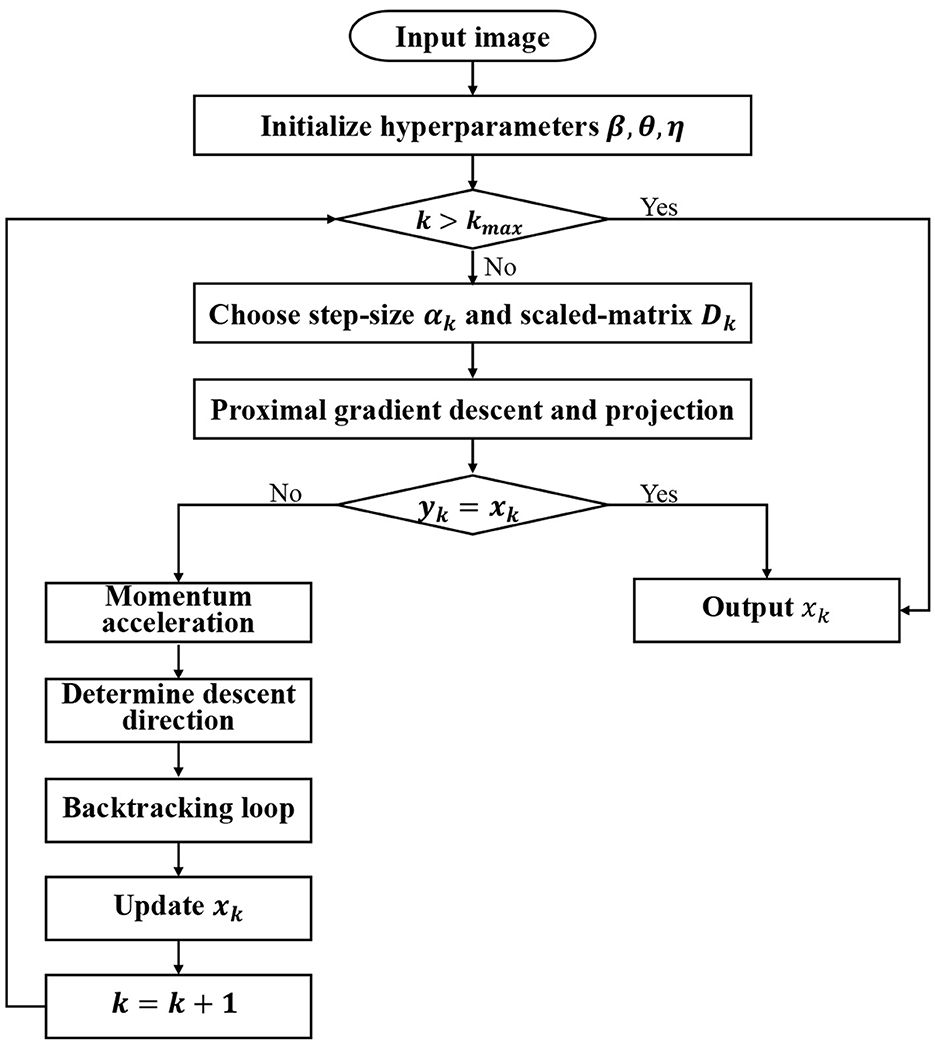
Figure 1. The flow diagram of the Algorithm 1.

Algorithm 1

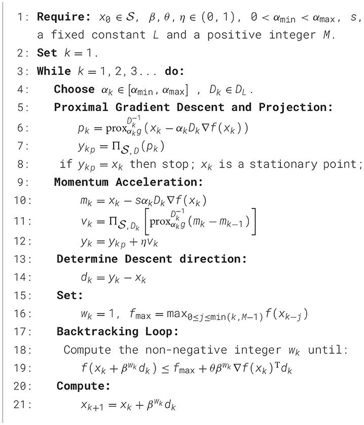
Algorithm 1. M-PSGP.

As illustrated in Figure 1, beyond parameter initialization, the algorithm primarily consists of four key computational phases, including proximal gradient descent and projection, momentum acceleration, determining the descent direction, and the backtracking loop. In the proximal gradient descent and projection step, the M-PSGP computes a gradient descent step on the smooth component f(x), then applies the proximal operator to account for the non-smooth regularizer g(x) in line 6. Subsequently, line 7 applies the projection operator to ensure constraint satisfaction. In the momentum acceleration step, the M-PSGP first computes the next intermediate position m_k, as shown in line 10. The calculation of momentum v_k is defined as m_k − m_k−1, and to satisfy the non-negative constraint, it should be projected as in line 11. The value v_k captures the change between successive intermediate positions during the optimization process. Thus, in line 12, the M-PSGP incorporates information about the past gradients into the update step, which helps accelerate and stabilize convergence toward the stationary point. Here, η is a hyperparameter that modulates the effect of momentum on the update direction. Subsequently, the descent direction is formally defined as the vector difference between the current iterate and the momentum-corrected candidate point in line 14. Finally, a backtracking line search loop in line 19 is executed to find an appropriate step size along this direction, which recalls the generalized non-monotone Armijo-type line search proposed by Zhang (2010).

In Figure 2, we present a schematic diagram of a single iteration for both the M-PSGP and SGP algorithms. To provide a more intuitive explanation, we present Table 1, which specifies the definitions of all nodes and vectors, along with their correspondences to the key steps of Algorithm 1. Based on the explanations provided in Table 1, we can conclude from Figure 2 that, under identical initial conditions, the E node (obtained by the M-PSGP algorithm) moves closer to the stationary point of F(x) after one iteration than the F node (obtained by the SGP algorithm). This observation further verifies, from a vector operation perspective, the acceleration effect of the M-PSGP algorithm. Additionally, it should be noted that, for the sake of clarity and conciseness, we have omitted explicit emphasis on projection operations, as all vectors are assumed to be constrained within the feasible domain by default. Likewise, nodes C and vector M₃ are also presented as the results obtained after applying the proximal operator.

Figure 2

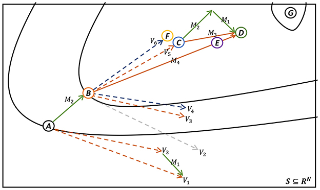
Figure 2. Iteration process of M-PSGP (accelerated by NAG) and SGP Algorithms. Nodes and vectors are noted in Table 1.

Table 1

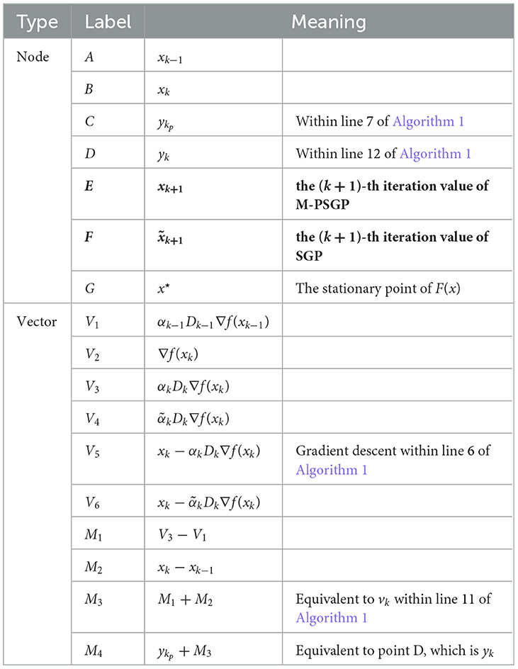
Table 1. Notation of nodes and vectors in Figure 2.

3.3 The improved step-size selection rule

In Algorithm 1, line 6 shows the proximal scaled gradient descent process under projection. Denote t_k = α_kD_k, which governs descent distance and affects the convergence rate during the solving process. In M-PSGP, we are committed to enhancing the selection strategy for the descent parameter t_k. The confirmation of D_k in M-PSGP corresponds to the rule (Equation 13) in SGP, which implies that an innovative t_k is contingent on a novel α_k strategy. In M-PSGP, tailored to the l₁-regularized problem (Equation 7), we propose a step-size rule BB2^* and a related SS^* rule to determine α_k, meanwhile, the descent parameter t_k is modified. As mentioned by Crisci et al. (2024), we consider the following partition of the index set during the iteration:

$\begin{array}{l}\begin{array}{l}{\mathcal{J}}_k=\left\{i:x_i^k=0\wedge -\nabla f(x_i^k)\in \partial (\lambda {\left|\right|·\left|\right|}_1)(x_i^k)\right\}\\ =\left\{i:x_i^k=0\wedge -\nabla f(x_i^k)\in \left[-\lambda ,\lambda \right]\right\},\\ {\mathcal{I}}_k=\left\{1,2,3,\dots ,n\right\} \backslash {\mathcal{J}}_k,\end{array}\end{array}$

where i denotes the index of the zero component in x_k. By invoking this partition in Algorithm 1, the iteration is carried out:

$\begin{array}{l}\begin{array}{c}{x}_i^{k+1}=\{\begin{array}{cc}0,& i\in {\mathcal{J}}_k,\\ x_i^k-{\beta }^{w_k}{\alpha }_k\left[\nabla f(x_i^k)+\text{sign}(t_k)·\lambda \right],& i\in {\mathcal{I}}_k,\end{array}\end{array}\end{array}$

in which t_k = x_k − α_kD_k ∇ f(x_k). Naturally, the vector s_k can be separated as:

$\begin{array}{ll}\begin{array}{c}{s}_k=\left[\begin{array}{c}{s}_{{\mathcal{J}}_k}\\ s_{{\mathcal{I}}_k}\end{array}\right]=\left[\begin{array}{c}0\\ -{\beta }^{w_k}{\alpha }_k\left[\nabla f(x_i^k)+\text{sign}(t_k)·\lambda \right]\end{array}\right],\end{array}& (20)\end{array}$

and the difference between the corresponding gradients z_k can be reformulated as:

$\begin{array}{ll}\begin{array}{c}{z}_k=\left[\begin{array}{c}{z}_{{\mathcal{J}}_k}\\ z_{{\mathcal{I}}_k}\end{array}\right]=\left[\begin{array}{c}{A}_{{\mathcal{J}}_k{\mathcal{I}}_k}{s}_{{\mathcal{I}}_k}\\ A_{{\mathcal{I}}_k{\mathcal{I}}_k}{s}_{{\mathcal{I}}_k}\end{array}\right].\end{array}& (21)\end{array}$

Applying Equations 20, 21 to the BB rules (Equation 14) and (Equation 15), we can obtain the following:

$\begin{array}{ll}{\alpha }_k^{\text{BB}1}=\frac{s_{{\mathcal{I}}_{k-1}}^{\text{T}}{D}_k^{-1}{D}_k^{-1}{s}_{{\mathcal{I}}_{k-1}}}{s_{{\mathcal{I}}_{k-1}}^{\text{T}}{D}_k^{-1}{z}_{{\mathcal{I}}_{k-1}}},& (22)\end{array}$

$\begin{array}{ll}{\alpha }_k^{\text{BB}2}=\frac{s_{{\mathcal{I}}_{k-1}}^{\text{T}}{D}_k{z}_{{\mathcal{I}}_{k-1}}}{z_{{\mathcal{I}}_{k-1}}^{\text{T}}{D}_k{D}_k{z}_{{\mathcal{I}}_{k-1}}+z_{{\mathcal{J}}_{k-1}}^{\text{T}}{D}_k{D}_k{z}_{{\mathcal{J}}_{k-1}}}.& (23)\end{array}$

Inspired by the BB2-like rule for box-constrained problems proposed by Crisci et al. (2019), we develop a new variant, which is termed the BB2^* rule, as follows:

$\begin{array}{ll}\begin{array}{c}{\alpha }_k^{\text{BB}{2}^{*}}=\frac{s_{{\mathcal{I}}_{k-1}}^{\text{T}}{D}_k{z}_{{\mathcal{I}}_{k-1}}}{z_{{\mathcal{I}}_{k-1}}^{\text{T}}{D}_k{D}_k{z}_{{\mathcal{I}}_{k-1}}}.\end{array}& (24)\end{array}$

Intuitively, the optimization process is accelerated by preemptively eliminating the optimal zero components, as the reciprocal of 1/α_k only depends on non-zero components. By excluding these zero components, the step-size calculation can focus on the active subspace, thereby improving the accuracy of curvature estimation, reducing redundant projections, and ultimately enhancing convergence efficiency. Furthermore, motivated by the SGP algorithm, which alternatively chooses α_k to balance convergence acceleration with algorithmic robustness, we determine α_k by switching between ${\alpha }_k^{\text{BB}{2}^{*}}$ and ${\alpha }_k^{\text{BB}1}$ adaptively. Thereafter, the comprehensive step-size selection rule, which we termed the SS^* rule, is defined as follows:

$\begin{array}{ll}{\alpha }_k=\{\begin{array}{lll}{\alpha }_k^{\text{BB}1},& if& \frac{{\alpha }_k^{\text{BB}1}}{{\alpha }_k^{\text{BB}{2}^{*}}}<\tau ,\\ {\alpha }_k^{\text{BB}{2}^{*}},& if& \frac{{\alpha }_k^{\text{BB}1}}{{\alpha }_k^{\text{BB}{2}^{*}}}\ge \tau ,\end{array}& (25)\end{array}$

where τ is the threshold determining the translation.

It is remarked that, since we propose a larger step-size rule BB2^* (Equation 24) than BB2 (Equation 15), it is possible that the y_kp after gradient descent and projection yields an opposite increase. In this situation, a monotone line search, which enforces the sequence f(x_k) to be strictly decreasing, might lead to multiple computation loops during backtracking. That results in a dissipation of the acceleration effect achieved by our BB2^* rule. Thus, equipping a non-monotone line search procedure is significant for the M-PSGP algorithm to adapt to the inherent non-monotonic nature of our step-size rules.

4 Computational complexity analysis and convergence analysis

In this section, we will focus on the computational complexity analysis and convergence analysis for the M-PSGP algorithm.

4.1 Computational complexity analysis

In our image deblurring problem, the dimension of the optimization variable is n = N = 65, 536 for 256 × 256 images. The point spread function (PSF) matrix A is typically a block circulant matrix with circulant blocks (BCCB). For such structured matrices, the matrix-vector product Ax can be computed with $\mathcal{O}$(nlogn) complexity by employing the fast Fourier transform (FFT) (Davis, 1979). Thus, the computational cost of major operations in one iteration of our M-PSGP algorithm is analyzed as follows:

• Gradient computation (T_∇): Computing $\nabla f(x_k)=A^{\top }(A{x}_k-y)$ requires two FFT-based operations, yielding $\mathcal{O}$(nlogn) complexity.

• Function evaluation (T_f): Evaluating $f(x_k)=\frac{1}{2}\left|\right|A{x}_k-y|{|}^2$ also requires FFT operations, with $\mathcal{O}$(nlogn) complexity.

• BB step-size computation (T_BB): Calculating α_k involves vector differences and inner products, requiring $\mathcal{O}$(n) operations.

• Diagonal scaling (T_D): Applying the diagonal scaling matrix D_k to vectors is an element-wise operation with $\mathcal{O}$(n) complexity.

• Proximal/projection operations (T_proj): Both the proximal operator for the ℓ₁-norm and the projection onto the non-negative orthant are element-wise operations with $\mathcal{O}$(n) complexity.

• Backtracking evaluations (N_bt): The average number of function evaluations during backtracking line search.

• Proximal calls (C_prox): The number of proximal/projection calls per iteration (typically C_prox = 2 in M-PSGP).

The overall per-iteration computational complexity can be expressed as follows:

$\begin{array}{ll}{T}_{\text{iter}}=T_{\nabla }+T_{\text{BB}}+T_D+C_{\text{prox}}{T}_{\text{proj}}+N_{\text{bt}}{T}_f+\mathcal{O}(n)& (26)\end{array}$

Substituting the respective complexities:

$\begin{array}{l}{T}_{\text{iter}}=\mathcal{O}(nlogn)+\mathcal{O}(n)+\mathcal{O}(n)+\mathcal{O}(n)+\mathcal{O}(nlogn)+\mathcal{O}(n)\\ =\mathcal{O}(nlogn)& (27)\end{array}$

Therefore, the per-iteration time complexity of the proposed M-PSGP algorithm is:

$\begin{array}{ll}\begin{array}{||}\hline T_{\text{iter}}=\mathcal{O}(n\log n)\\ \hline\end{array}& (28)\end{array}$

The $\mathcal{O}$(nlogn) term dominates due to the FFT-based gradient and function evaluations, while all other operations maintain linear $\mathcal{O}$(n) complexity. This complexity is significantly more efficient than the $\mathcal{O}$(n²) complexity required by direct matrix operations, making our algorithm suitable for high-dimensional image processing problems.

4.2 Convergence analysis

In this section, we will focus on the convergence analysis for the M-PSGP algorithm. The main convergence guarantee of M-PSGP in the case of heavy-ball momentum acceleration is presented in Theorem 1, and its proof is based on a series of basic properties that we state in the following lemmas.

Lemma 4. Assume that y_k ≠ x_k, then, the d_k = y_k − x_k is a strict descent direction for the function f at x_k, that is, $\nabla f{(x_k)}^{\text{T}}{d}_k<0$.

Proof. The proof of this lemma is detailed in Appendix A.     □

Lemma 5. Define e_k = m_k − x_k, where m_k = x_k − sα_kD_k ∇ f(x_k), it has:

$\begin{array}{ll}\left|\right|e_k\left|\right|\le s{\alpha }_{\text{max}}LG,& (29)\end{array}$

for ||D_k|| ≤ L, α_k ∈ [α_min, α_max] and G = max_{x ∈ $\mathcal{S}$}||∇f(x)||.

Proof. The proof of this lemma is detailed in Appendix B.

Lemma 6. Consider a Lyapunov function ${\text{Ψ}}_k=F(x)+\frac{\rho }{2{\alpha }_k}\left|\right|e_k|{|}^2$, where F(x) is constructed as Equation 7 and ||e_k|| is defined as (29). There exist constants σ, ρ > 0 such that:

$\begin{array}{l}{\text{Ψ}}_{k+1}\le {\text{Ψ}}_k-\sigma {\beta }^{w_k}|\nabla f{(x_k)}^{\text{T}}{d}_k|,k=1,2,\dots \end{array}$

Proof. The proof of this lemma is detailed in Appendix C.

Lemma 7. Let β ∈ (0, 1) and θ ∈ (0, 1) be fixed constants. For any iteration k, the nonmonotone backtracking line search terminates in a finite number of trials; that is, there exists w_k > 0 such that the following inequality holds:

$\begin{array}{l}f(x_k+{\beta }^{w_k}{d}_k)\le f_{\text{max}}+\theta {\beta }^{w_k}\nabla f{(x_k)}^{\text{T}}{d}_k,\end{array}$

where f_max = max_{0 ≤ j ≤ min(k, M−1)}f(x_k−j).

Proof. The proof of this lemma is detailed in Appendix D.

Theorem 1. Consider the composite convex minimization problem (Equation 7) and suppose the sequence {x_k} is generated by the M-PSGP algorithm under the assumption that the level set {x:F(x) ≤ F(x₀)} is bounded. Then the sequence {x_k} converges to a stationary point x^* of F over $\mathcal{S}$ = {x : x ≥ 0}, i.e.,

$\begin{array}{l}{\displaystyle \underset{k\to \infty }{lim}}{x}_k=x^{*}.\end{array}$

Proof. The proof of this theorem is detailed in Appendix E.

5 Results

In this section, we conduct simulation experiments to confirm the superiority of the M-PSGP algorithm in solving l₁-regularized optimization problems, with a focus on its application to image deblurring. All algorithms are implemented in Python 3.8.10, and the experiments are conducted on a computer equipped with a 12th Gen Intel(R) Core(TM) processor at 2.30 GHz.

First, we compare the performance of different BB-like step-size rules within the framework of the SGP algorithm, demonstrating the superiority of SS^* rules in accelerating the convergence rate and enhancing deblurring effectiveness. For the sake of convenience in notation, we name the method that incorporates SS^* into SGP as the SGP* algorithm. Then, we combine the unified momentum framework UM with the SGP* algorithm, which serves as the M-PSGP algorithm. The comparison between the SGP* and M-PSGP demonstrates the notable advantage of momentum acceleration. Moreover, we compare M-PSGP with other seminal methods and present its excellence.

5.1 Experiment settings and performance measures

All of the algorithms are tested on problem (Equation 7). The test examples are generated by convolving the original 256 × 256 images with the Gaussian kernels of different noise levels (σ² = 5 and σ² = 10; higher σ values result in stronger blurring effects), followed by additive white noise with a Gaussian distribution (σ² = 0.01). To ensure an objective and consistent evaluation of the proposed M-PSGP algorithm and its comparison with the baseline SGP method, we adopted the test examples used in Bonettini and Prato (2015); Federica et al. (2015) and selected two representative CT images. Furthermore, to comprehensively evaluate the generalization capability and robustness of the M-PSGP algorithm, we also selected four images of different types from the standard image processing benchmark dataset Set12 proposed by Zhang et al. (2017) as supplementary test examples. The complete set of selected test examples is presented in Figure 3.

Figure 3

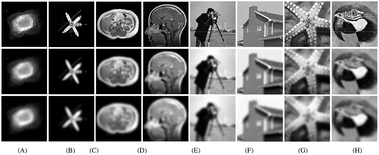
Figure 3. Test examples. The first row displays the original images, the second row displays the deblurred images with σ² = 5, the third row displays the deblurred images with σ² = 10. The test images are sequentially labeled as: (A) NGC7027; (B) SATELLITE; (C) CHAOS; (D) OASIS; (E) CAMERAMAN; (F) HOUSE; (G) FISHSTAR; (H) PARROT.

To evaluate and compare the effectiveness of different algorithms, we measure the number of convergence iterations (ITER), the corresponding runtime (TIME) to achieve convergence, relative reconstruction error (RRE) (Bonettini et al., 2008), peak signal-to-noise ratio (PSNR) (Liao et al., 2025), and structural similarity (SSIM) (Liao et al., 2024). These indicators are defined as follows:

$\begin{array}{l}\text{RRE}=\frac{\left|\right|\widehat{x}-x\left|\right|}{\left|\right|x\left|\right|},\\ \text{PSNR}=10lo{g}_{10}\frac{255^2\times M\times N}{{\displaystyle {\sum }_{m=1}^M}{\displaystyle {\sum }_{n=1}^N}{(x_{m,n}-{\widehat{x}}_{m,n})}^2},\\ \text{SSIM}=\frac{(2{\mu }_x{\mu }_{\widehat{x}}+c_1)(2{\sigma }_{x\widehat{x}}+c_2)}{({\mu }_x^2+{\mu }_{\widehat{x}}^2+c_1)({\sigma }_x^2+{\sigma }_{\widehat{x}}^2+c_2)},\end{array}$

where x is the original image and $\widehat{x}$ is the deblurred image, M and N denote the sizes along the two dimensions of the image. μ_x and ${\mu }_{\widehat{x}}$ are the pixel-wise averages, σ_x and ${\sigma }_{\widehat{x}}$ are the variances of x and $\widehat{x}$, ${\sigma }_{x\widehat{x}}$ is the covariance between x and $\widehat{x}$, and c₁ and c₂ are stability constants.

In all simulations, we set the maximum number of iterations as 200, ${\alpha }_{min}=10^{-10}$, ${\alpha }_{max}=10^5$, and α₀ = 1.3. The step size threshold τ is set as 0.15. In the backtracking loop step, the line search parameters are θ = 10⁻⁴, β = 0.95. The initial iteration value x₀ is set as follows: $x_i^0=\frac{\sum _{i=1}^N{y}_i}{N}(i=1,2,3,\cdots ,N),$ where y are the observed values.

5.2 Comparison of step-size rules in SGP

In this subsection, we inspect the performance in practical implementations of those different step-size rules:

• BB1: ${\alpha }_k={\alpha }_k^{\text{BB}1}$, where ${\alpha }_k^{\text{BB}1}$ is defined as the rule (Equation 14).

• BB2: ${\alpha }_k={\alpha }_k^{\text{BB}2}$, where ${\alpha }_k^{\text{BB}2}$ is defined as the rule (Equation 15).

• SS: α_k is defined following the SS algorithm proposed by Bonettini and Prato (2015).

• BB2^*: α_k is defined following the rule (Equation 24).

• SS^*: α_k is defined following the rule (Equation 25).

Here, the BB2^* and SS^* are our proposed rules. To adhere to the principle of a single variable, thereby enhancing the referential value of the experimental outcomes, we uniformly implement these rules in the SGP algorithm.

The numerical results are reported in Table 2 and Figure 4. Table 2 shows that for all test images, SS^* could achieve the highest PSNR and SSIM on all test images, indicating the best optimization effect and the highest quality of the reconstructed images. As shown in the curve in Figure 4, it can be concluded that SS^* and BB2^* require fewer iterations to achieve the same effect compared to other rules at the preliminary iteration stage, which means that the SS^* and BB2^* rules can improve the convergence rate more than other rules. Across the comprehensive optimization stages, SS^* achieves the lowest RRE (the highest negative logarithm of RRE), demonstrating the dual advantages of SS^* in accelerating convergence while enhancing optimization accuracy. Indeed, the SGP algorithm employing the SS* method is equivalent to the M-PSGP algorithm operating without its momentum acceleration, which can be denoted as the SGP* algorithm.

Table 2

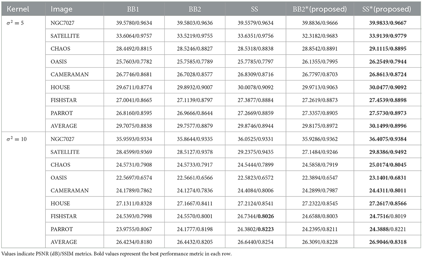
Table 2. Performance comparison of different step-size rules under various noise levels (σ² = 5 and σ² = 10).

Figure 4

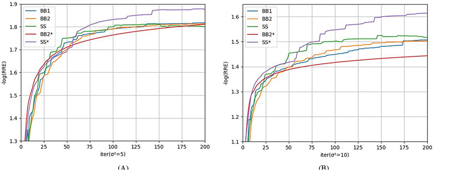
Figure 4. Comparison of different step-size rules in terms of the average negative logarithm of RRE: (A) σ² = 5; (B) σ² = 10.

5.3 Comparison between SGP* and M-PSGP

Aiming to study the acceleration and stability effects of the unified momentum framework UM (Equation 16), we compare the M-PSGP algorithm with the SGP^* algorithm (M-PSGP without its momentum acceleration) in this subsection. Table 3 presents the numerical performance of SGP^* and M-PSGP variants (accelerated by HB, NAG, and GM). The results demonstrate that all M-PSGP variants can produce more efficient results than SGP^*. From Figure 5, we can observe that the M-PSGP variants consistently outperform SGP^* in convergence speed across noise levels, achieving faster RRE reduction and earlier stabilization. Furthermore, as shown in Equation 16, the selection of parameter η must satisfy the range required for the convergence of the algorithms, and then within this range, values that yield higher performance metrics are chosen. To demonstrate the sensitivity of η, using the NGC7027 case with a blur level of σ² = 5 as an example, we investigated the performance of three accelerated variants (HB: s = 0, NAG: s = 1, and GM: s = 1/1 − η) under different values of the parameter η. Using the NGC7027 case with a blur level of σ² = 5 as an example. The experimental results are presented in Figure 6.

Table 3

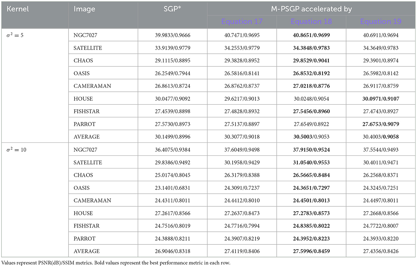
Table 3. Performance comparison between SGP* and M-PSGP accelerated variants under different noise levels (σ² = 5 and σ² = 10).

Figure 5

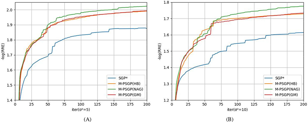
Figure 5. Comparison between SGP* and M-PSGP accelerated variants in terms of the average negative logarithm of RRE: (A) σ² = 5; (B) σ² = 10.

Figure 6

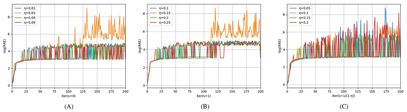
Figure 6. Sensitivity and optimal choice of η for M-PSGP accelerated variants: (A) s = 0; (B) s = 1; (C) s = 1/(1 − η).

5.4 Comparison of M-PSGP with other algorithms

In this subsection, we present the comparison of the M-PSGP algorithm with other algorithms, including TwIST (Bioucas-Dias and Figueiredo, 2007), FISTA (Beck and Teboulle, 2009), SGP (Bonettini and Prato, 2015), OptISTA (Jang et al., 2025), and IOptISTA (Wang et al., 2025). Table 4 presents the performance metrics of M-PSGP and other seminal algorithms, from which we can conclude that M-PSGP achieves the highest PSNR and SSIM, among others. On 12 out of the 16 test examples, the M-PSGP algorithm achieved satisfactory deblurring performance in less time, which is attributed to its requiring fewer iterations to converge. On the remaining four test images, M-PSGP achieved better deblurring performance under the same iteration limit, albeit at the expense of a longer total runtime. In Figure 7, based on the average variations in curvature depicted, we further substantiate that the M-PSGP algorithm can accelerate convergence during the optimization process more than others. In Figure 8, we present a magnified view of the deblurring effects on test images under the Gaussian noise level σ² = 5, which allows for a visual assessment of the M-PSGP and other algorithms. The magnified details demonstrate the superior capabilities of the M-PSGP algorithm in enhancing the overall effect of image deblurring, as well as in preserving and clarifying edges.

Table 4

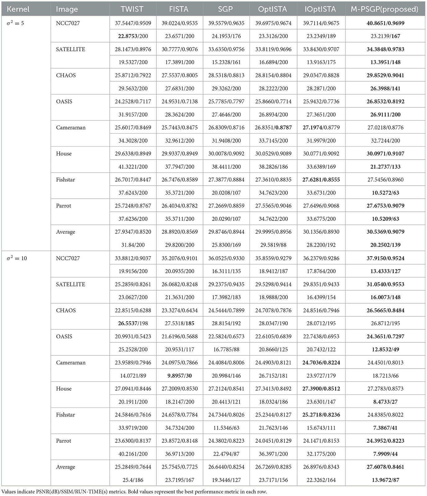
Table 4. Performance comparison of different deblurring algorithms under various noise levels (σ² = 5 and σ² = 10).

Figure 7

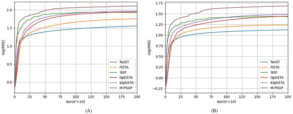
Figure 7. Comparison of TwIST, FISTA, SGP, OptISTA, IoptISTA and M-PSGP in terms of the average negative logarithm of RRE: (A) σ² = 5; (B) σ² = 10.

Figure 8

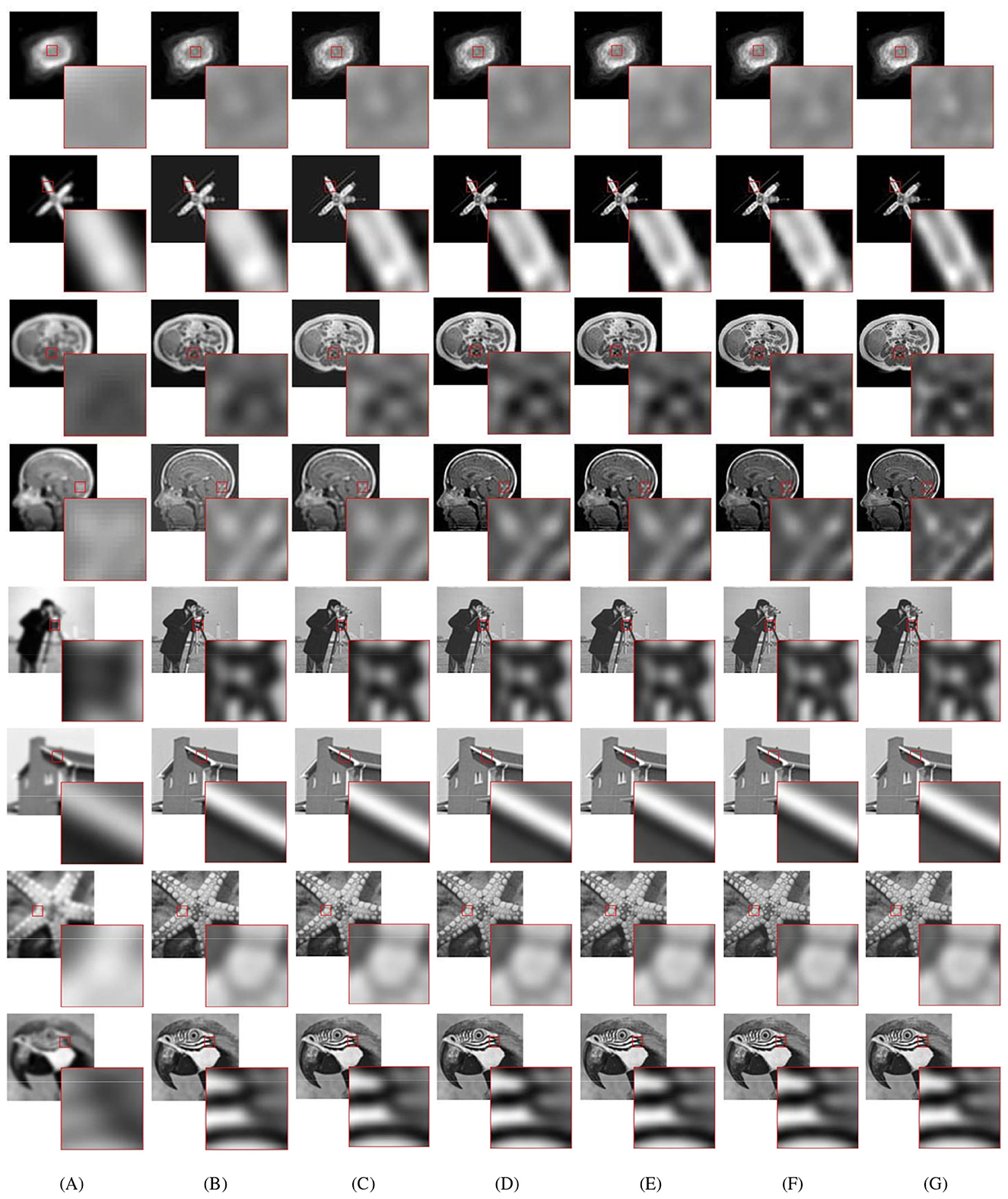
Figure 8. Visual reconstructed results from blurred test images (σ² = 5). The images shown from left to right are (A) blurred images; (B) TWIST-deblurred images; (C) FISTA-deblurred images; (D) SGP-deblurred images; (E) OptISTA-deblurred images; (F) IoptISTA-deblurred images; (G) M-PSGP-deblurred images.

6 Conclusion and discussion

In this study, we propose the M-PSGP algorithm and demonstrate its significant improvement in optimizing l₁-regularized problems, with applications to image deblurring. The integration of the improved step-size rule BB2^* and the unified momentum framework UM has led to accelerated convergence rates and improved performance in image deblurring tasks. Numerical experiments have demonstrated that the M-PSGP algorithm outperforms existing proximal gradient projection algorithms, TwIST, FISTA, SGP, OptISTA, and IOptISTA. The M-PSGP algorithm has presented a credible alternative to conventional techniques in image deblurring and has demonstrated potential applications in other domains, where l₁-regularized optimization problems are prevalent. In the future, we will endeavor to apply the M-PSGP algorithm to other optimization problems, such as ridge regression and non-convex optimization, thereby enhancing its applicability to a broader range of signal processing tasks. Furthermore, with the potential to provide novel perspectives for tackling large-scale optimization problems, the application of the M-PSGP algorithm to parameter training in machine learning is also a significant research topic.

While this study presents a promising optimization framework, its practical deployment may face certain limitations that warrant further discussion. First, the performance of the method depends on the selection of several hyperparameters (e.g., η). Although the algorithm incorporates adaptive mechanisms, its sensitivity to these settings may present challenges in practical applications, where parameter tuning is limited or robustness is essential. Second, the convergence analysis and numerical experiments are conducted under standard assumptions. The method's performance in non-Gaussian or heavy-tailed noise environments remains an open question. Such conditions are common in real-world data (e.g., sensor data), and the robustness of momentum acceleration and line search strategies in these settings warrants further investigation. Acknowledging these aspects would provide a more comprehensive view of the method's operational scope and guide future research toward enhancing its practical robustness and applicability.

Data availability statement

The original contributions presented in the study are included in the article/Supplementary material, further inquiries can be directed to the corresponding author.

Author contributions

KN: Formal analysis, Investigation, Methodology, Visualization, Writing – original draft, Writing – review & editing. QL: Conceptualization, Formal analysis, Investigation, Methodology, Supervision, Writing – original draft, Writing – review & editing. XL: Funding acquisition, Resources, Supervision, Writing – original draft, Writing – review & editing.

Funding

The author(s) declare that financial support was received for the research and/or publication of this article. This work was supported in part by the Natural Science Foundation of Chongqing (Innovation and Development Joint Fund) under Grants CSTB2023NSCQ-LZX0149 and CSTB2025NSCQ-LZX0085, in part by the Graduate Research and Innovation Foundation of Chongqing under Grant CYB25038, and in part by the National Natural Science Foundation of China under Grants 62576053 and 62302068.

Conflict of interest

The authors declare that the research was conducted in the absence of any commercial or financial relationships that could be construed as a potential conflict of interest.

Generative AI statement

The author(s) declare that no Gen AI was used in the creation of this manuscript.

Any alternative text (alt text) provided alongside figures in this article has been generated by Frontiers with the support of artificial intelligence and reasonable efforts have been made to ensure accuracy, including review by the authors wherever possible. If you identify any issues, please contact us.

Publisher's note

All claims expressed in this article are solely those of the authors and do not necessarily represent those of their affiliated organizations, or those of the publisher, the editors and the reviewers. Any product that may be evaluated in this article, or claim that may be made by its manufacturer, is not guaranteed or endorsed by the publisher.

Supplementary material

The Supplementary Material for this article can be found online at: https://www.frontiersin.org/articles/10.3389/fdata.2025.1704189/full#supplementary-material

References

Aravkin, A., Baraldi, R., and Orban, D. (2022). A proximal quasi-newton trust-region method for nonsmooth regularized optimization. SIAM J. Optim. 32, 900–929. doi: 10.1137/21M1409536

Crossref Full Text | Google Scholar

Barzilai, J., and Borwein, J. (1988). Two-point step size gradient methods. IMA J. Numer. Anal. 8, 141–148. doi: 10.1093/imanum/8.1.141

Crossref Full Text | Google Scholar

Bauschke, H., and Combettes, P. (2017). Correction to: Convex Analysis and Monotone Operator Theory in Hilbert Spaces. Cham: Springer. doi: 10.1007/978-3-319-48311-5

Crossref Full Text | Google Scholar

Beck, A., and Teboulle, M. (2009). A fast iterative shrinkage-thresholding algorithm for linear inverse problems. SIAM J. Imaging Sci. 2, 183–202. doi: 10.1137/080716542

Crossref Full Text | Google Scholar

Bioucas-Dias, J., and Figueiredo, M. (2007). A new twist: two-step iterative shrinkage/thresholding algorithms for image restoration. IEEE Trans. Image Process 16, 2992–3004. doi: 10.1109/TIP.2007.909319

PubMed Abstract | Crossref Full Text | Google Scholar

Bonettini, S., and Prato, M. (2015). New convergence results for the scaled gradient projection method. Inverse Probl. 31:095008. doi: 10.1088/0266-5611/31/9/095008

Crossref Full Text | Google Scholar

Bonettini, S., Zanella, R., and Zanni, L. (2008). A scaled gradient projection method for constrained image deblurring. Inverse Probl. 25:015002. doi: 10.1088/0266-5611/25/1/015002

Crossref Full Text | Google Scholar

Chen, X., Cheng, D., and Feng, J. (2025). Matrix projection and its application in image processing. Digital Signal Process 163:105231. doi: 10.1016/j.dsp.2025.105231

Crossref Full Text | Google Scholar

Crisci, S., Rebegoldi, S., Toraldo, G., and Viola, M. (2024). Barzilai-borwein-like rules in proximal gradient schemes for l1-regularized problems. Optim. Methods. Softw. 39, 601–633. doi: 10.1080/10556788.2023.2285489

Crossref Full Text | Google Scholar

Crisci, S., Ruggiero, V., and Zanni, L. (2019). Steplength selection in gradient projection methods for box-constrained quadratic programs. Appl. Math. Comput. 356, 312–327. doi: 10.1016/j.amc.2019.03.039

Crossref Full Text | Google Scholar

Davis, P. J. (1979). Circulant Matrices, Vol. 120. New York, NY: Wiley.

Google Scholar

Du, H., Cheng, C., and Ni, C. (2024). A unified momentum-based paradigm of decentralized sgd for non-convex models and heterogeneous data. Artif. Intell. 332:104130. doi: 10.1016/j.artint.2024.104130

Crossref Full Text | Google Scholar

Federica, P., Marco, P., and Luca, Z. (2015). A new steplength selection for scaled gradient methods with application to image deblurring. J. Sci. Comput. 65, 895–919. doi: 10.1007/s10915-015-9991-9

Crossref Full Text | Google Scholar

He, C., Zhang, Y., Zhu, D., Cao, M., and Yang, Y. (2023). A mini-batch algorithm for large-scale learning problems with adaptive step size. Digit. Signal Process 143:104230. doi: 10.1016/j.dsp.2023.104230

Crossref Full Text | Google Scholar

Jang, U., Gupta, S., and Ryu, E. (2025). Computer-assisted design of accelerated composite optimization methods: optista. Math. Programm. 1–109. doi: 10.1007/s10107-025-02258-5

Crossref Full Text | Google Scholar

Liao, X., Wei, X., Zhou, M., Li, Z., and Kwong, S. (2024). Image quality assessment: measuring perceptual degradation via distribution measures in deep feature spaces. IEEE Trans. Image Process. 33, 4044–4059. doi: 10.1109/TIP.2024.3409176

PubMed Abstract | Crossref Full Text | Google Scholar

Liao, X., Wei, X., Zhou, M., Wong, H., and Kwong, S. (2025). Image quality assessment: Exploring joint degradation effect of deep network features via kernel representation similarity analysis. IEEE Trans. Pattern Anal. Mach. Intell. 47, 2799–2815. doi: 10.1109/TPAMI.2025.3527004

PubMed Abstract | Crossref Full Text | Google Scholar

Liu, R., Sun, W., Hou, T., Hu, C., and Qiao, L. (2019). Block coordinate descent with time perturbation for nonconvex nonsmooth problems in real-world studies. Front. Inform. Technol. Electron. Eng. 20, 1390–1403. doi: 10.1631/FITEE.1900341

Crossref Full Text | Google Scholar

Loizou, N., and Richtárik, P. (2020). Momentum and stochastic momentum for stochastic gradient, newton, proximal point and subspace descent methods. Comput. Optim. Appl. 77, 653–710. doi: 10.1007/s10589-020-00220-z

Crossref Full Text | Google Scholar

Malitsky, Y., and Mishchenko, K. (2024). “Adaptive proximal gradient method for convex optimization,” in Proc Adv Neural Inf Process Syst (Red Hook, NY Curran Associates, Inc), 100670–100697. doi: 10.52202/079017-3193

Crossref Full Text | Google Scholar

Maroni, G., Cannelli, L., and Piga, D. (2025). Gradient-based bilevel optimization for multi-penalty ridge regression through matrix differential calculus. Eur. J. Control. 81, 101150. doi: 10.1016/j.ejcon.2024.101150

Crossref Full Text | Google Scholar

Nesterov, Y. (1983). A method for solving the convex programming problem with convergence rate o(1/k²). Proc. Dokl. Akad. Nauk. SSSR 269543.

Google Scholar

Parikh, N., and Boyd, S. (2014). Proximal algorithms. Found. Trends Optim. 1, 127–239. doi: 10.1561/2400000003

Crossref Full Text | Google Scholar

Polyak, B. (1964). Some methods of speeding up the convergence of iteration methods. USSR Comput. Math. Math. Phys. 4, 1–17. doi: 10.1016/0041-5553(64)90137-5

Crossref Full Text | Google Scholar

Tang, X., Zhao, X., Liu, J., Wang, J., Miao, Y., Zeng, T., et al. (2023). “Uncertainty-aware unsupervised image deblurring with deep residual prior,” in Proceedings of the IEEE/CVF Conference on Computer Vision and Pattern Recognition, 9883–9892. doi: 10.1109/CVPR52729.2023.00953

Crossref Full Text | Google Scholar

Wang, D. (2025). Monotonically accelerated proximal gradient for nonnegative tensor decomposition. Digital Signal Process 161, 105097. doi: 10.1016/j.dsp.2025.105097

Crossref Full Text | Google Scholar

Wang, Q., Xu, S., Tong, X., and Zeng, T. (2025). An improved optimal proximal gradient algorithm for non-blind image deblurring. arXiv [preprint]. arXiv:2502.07602. doi: 10.48550/arXiv:2502.07602

Crossref Full Text | Google Scholar

Xie, Z., Liu, L., Chen, Z., and Wang, C. (2025). Proximal gradient algorithm with dual momentum for robust compressive sensing MRI. Signal Process. 230:109817. doi: 10.1016/j.sigpro.2024.109817

Crossref Full Text | Google Scholar

Yang, T., Lin, Q., and Li, Z. (2016). Unified convergence analysis of stochastic momentum methods for convex and non-convex optimization. arXiv [preprint]. arXiv:1604.03257. doi: 10.48550/arXiv.1604.03257

Crossref Full Text | Google Scholar

Zhang, J. (2010). “On the non-monotone armijo-type line search algorithm,” in Proc Int Conf on Inf and Comput., Vol. 3 (Wuxi: IEEE), 308–311. doi: 10.1109/ICIC.2010.263

Crossref Full Text | Google Scholar

Zhang, J., Zhang, G., Liang, Z., and Liao, L. (2023). Momentum acceleration-based matrix splitting method for solving generalized absolute value equation. Appl. Math. Comput. 42:300. doi: 10.1007/s40314-023-02436-1

Crossref Full Text | Google Scholar

Zhang, K., Zuo, W., Chen, Y., Meng, D., and Zhang, L. (2017). Beyond a gaussian denoiser: Residual learning of deep cnn for image denoising. IEEE Trans. Image Process. 26, 3142–3155. doi: 10.1109/TIP.2017.2662206

PubMed Abstract | Crossref Full Text | Google Scholar

Zhou, Q., Qian, J., Yang, Z., Huang, C., Chen, Q., Xu, Y., et al. (2025). Robust wideband waveform design with constant modulus and discrete phase constraints for distributed precision jamming. Front. Inform. Technol. Electron. Eng. 26, 119–133. doi: 10.1631/FITEE.2400285

Crossref Full Text | Google Scholar