Posterior averaging with Gaussian naive Bayes and the R package RandomGaussianNB for big-data classification

RandomGaussianNB is an open-source R package implementing the posterior-averaging Gaussian naive Bayes (PAV-GNB) algorithm, a scalable ensemble extension of the classical GNB classifier. The method introduces posterior averaging to mitigate correlation bias and enhance stability in high-dimensional settings while maintaining interpretability and computational efficiency. Theoretical results establish the variance of the ensemble posterior, which decreases inversely with ensemble size, and a margin-based generalization bound that connects posterior variance with classification error. Together, these results provide a principled understanding of the bias–variance trade-off in PAV-GNB. The package delivers a fully parallel, reproducible framework for large-scale classification. Simulation studies under big-data conditions—large samples, many features, and multiple classes—show consistent accuracy, low variance, and agreement with theoretical predictions. Scalability experiments demonstrate near-linear runtime improvement with multi-core execution, and a real-world application on the Pima Indians Diabetes dataset validates PAV-GNB's reliability and computational efficiency as an interpretable, statistically grounded approach for ensemble naive Bayes classification.

1 Introduction

Machine learning has become a cornerstone of modern data-driven research, advancing pattern recognition, classification, and forecasting across domains such as natural language processing, healthcare, and energy systems. Deep-learning architectures like convolutional and recurrent neural networks (LeCun et al., 1998; Hochreiter and Schmidhuber, 1997) have achieved remarkable results, yet their success depends on vast data, intensive hyper-parameter tuning, and substantial computational resources. These requirements remain prohibitive in many practical settings, prompting renewed interest in lightweight algorithms that balance accuracy, interpretability, and scalability (Mahmud et al., 2020; Wang Y. et al., 2020; Tantalaki et al., 2020; Liapis et al., 2023).

Among these, the Naive Bayes (NB) classifier stands out for its simplicity and robustness. Despite its conditional-independence assumption, NB achieves competitive performance in text analytics, bioinformatics, and medical diagnostics (Rish, 2001; Jurafsky and Martin, 2008; Wang et al., 2007). Decades of work have refined NB through improved probability estimation, semi-parametric treatment of continuous features, and Bayesian-network generalizations (Domingos and Pazzani, 1997; Zhang H., 2004; Zhang T., 2004; Rennie et al., 2003). Empirical studies show that the Gaussian Naive Bayes (GNB) variant often performs well even when assumptions are violated, as feature-wise errors can offset one another (Hand and Yu, 2001; Soria et al., 2011). However, real-world data frequently deviate from Gaussianity, exhibiting skewness or heavy tails that reduce accuracy (Boulle, 2007).

To address these issues, researchers have developed distribution-aware extensions such as alpha-skew GNB (Ara and Louzada, 2022) and t- or stable-distribution NB models that improve robustness to asymmetry and outliers (Bhamre et al., 2025). Ensemble-based variants, including randomized-feature and bootstrap-enhanced NB, enhance predictive stability without adding complexity (Phatcharathada and Srisuradetchai, 2025). These exploit stochastic diversity among resampled datasets and feature subsets to jointly reduce bias and variance—a principle central to the present work.

A further limitation of GNB is its conditional-independence assumption. Copula-based formulations relax this constraint by modeling dependencies among marginals, improving accuracy under correlated features (Elidan, 2012; Wang B. et al., 2020). Non-parametric variants, which replace Gaussian likelihoods with kernel-density estimators, flexibly capture arbitrary feature distributions (Boli and Wei, 2024; Shawe-Taylor and Cristianini, 2004). Together, these advances show that enriching NB with randomization, dependency modeling, or non-parametric estimation enhances generalization and calibration.

Ensemble methods such as bagging (Breiman, 1996), boosting (Schapire, 2003; Freund and Schapire, 1997), random subspaces (Ho, 1998), and random forests (Breiman, 2001) demonstrate how aggregating weak learners mitigates variance and bias (Polikar, 2006; Zhou, 2012; Dietterich and Kong, 1995). Building on these principles, Phatcharathada and Srisuradetchai (2025) proposed the randomized feature–bootstrapped naive Bayes (RFB-NB) algorithm, combining bootstrap aggregation and random feature selection to reduce correlation bias and improve calibration. Although that study established the empirical feasibility of the approach, it lacked formal theoretical analysis, generalization proofs, and a reproducible parallel implementation.

We address these gaps by developing the posterior-averaging Gaussian naive Bayes (PAV-GNB) algorithm and its open-source RandomGaussianNB R package. This study formalizes both the theoretical and algorithmic foundations of PAV-GNB, establishing its variance-reduction and generalization properties while delivering a scalable, parallel, and reproducible framework for high-dimensional classification.

The remainder of this paper is organized as follows. Section 2 reviews related work on Naive Bayes, randomized feature selection, and bootstrap ensembles. Section 3 introduces the proposed PAV-GNB algorithm and its theoretical analysis (Section 3.2), along with the benchmarking design and evaluation metrics. Section 4 presents empirical results, Section 5 details the RandomGaussianNB R package implementation, and Section 6 concludes with key findings and future directions.

2 Related theory and literature review

This study builds on the RFB-NB algorithm by Phatcharathada and Srisuradetchai (2025), which combines Gaussian naive Bayes (GNB) with random subspace and bootstrap aggregation. While their approach uses majority voting, we propose averaged class probabilities, where posterior probabilities are averaged across the ensemble to reduce correlation bias and improve stability. This work re-implements their framework in R, enabling reproducibility, scalability testing, and integration into R-based workflows. This section briefly reviews the theoretical foundations of GNB, randomized feature selection, and bootstrap ensemble learning, followed by a discussion of available NB software tools.

2.1 Gaussian naive Bayes

NB remains widely used for classification due to its interpretability, simplicity, and computational efficiency (Pearl, 1988; Bishop, 2006; Barber, 2012). The method is grounded in Bayes' theorem and assumes conditional independence of features given the class. A widely applied variant is GNB, designed for continuous-valued features. In GNB, each feature within a class is assumed to follow a Gaussian distribution. Mathematically, for a vector of features x = (x₁, x₂, …, x_p), the posterior probability that x belongs to class C_k is given by

$\begin{array}{ll}P(C_k|\text{x})=\frac{P(C_k){\prod }_{j=1}^{p}P(x_j|C_k)}{{\sum }_{i=1}^{K}P(C_i){\prod }_{j=1}^{p}P(x_j|C_i)},& (1)\end{array}$

where K denotes the number of classes and p the number of features (Murphy, 2012; McCallum and Nigam, 1998). The posterior probability in (1) defines the fundamental Bayesian decision rule for Gaussian naive Bayes. Under the Gaussian assumption, each conditional likelihood takes the form:

$\begin{array}{ll}P(x_j|C_k)=\frac{1}{\sqrt{2\pi {\sigma }_{jk}^2}}exp\left(-\frac{{(x_j-{\mu }_{jk})}^2}{2{\sigma }_{jk}^2}\right),& (2)\end{array}$

where μ_jk and ${\sigma }_{jk}^2$ denote the mean and variance of feature j within class C_k, respectively. Each class-conditional Gaussian likelihood in (2) specifies how continuous features contribute to posterior computation.

Despite its efficiency and practical success across tasks such as text classification and medical diagnostics, the independence assumption limits GNB's performance in real-world settings where correlations among features are common. These correlations often degrade predictive accuracy, motivating extensions that relax this assumption or combine GNB with ensemble and feature-randomization techniques (Rennie et al., 2003; Friedman et al., 1997).

2.2 Randomized feature selection and feature reduction methods

Feature selection and reduction methods aim to identify informative subsets of variables from the original feature space, thereby improving predictive performance, interpretability, and computational efficiency (Li et al., 2017). Formally, given an initial feature set, shown in (3).

$\begin{array}{ll}F=\left\{F_1,F_2,...,F_p\right\},& (3)\end{array}$

where p denotes the total number of available features, the objective is to find an optimal subset F^* ⊆ F that maximizes a criterion function J(·):

$\begin{array}{ll}{F}^{*}={\displaystyle \underset{F^{\prime }\subseteq F}{argmax}}J(F^{\prime }),& (4)\end{array}$

where J(F′) may represent predictive accuracy, information gain, or another performance-based criterion (Hall, 1999). The optimization criterion J(F′) in (4) captures predictive relevance or mutual information. Wrapper methods explicitly evaluate subsets through resampling or cross-validation (Guyon and Elisseeff, 2003), while filter methods employ statistical measures such as correlation or mutual information to eliminate redundant and irrelevant variables (Urbanowicz et al., 2018).

Beyond deterministic approaches, randomized feature selection introduces controlled stochasticity to diversify ensembles and mitigate feature correlations. At each iteration t, a random subset

$\begin{array}{ll}{F}_t=\left\{F_{t_1},F_{t_2},...,F_{t_m}\right\},m\ll p& (5)\end{array}$

is drawn without replacement from the full feature set. Repeating this process across T iterations yields a collection of subsets {F₁, F₂, ..., F_T}, each serving as the basis for training a classifier (Dietterich, 2000; Biau and Scornet, 2016; Sagi and Rokach, 2018). Randomized feature subsets in (5) diversify the ensemble, reducing correlation among base learners.

Decision-tree-guided approaches, proposed by Ratanamahatana and Gunopulos (2003), use decision tree classifiers to recursively partition the feature space, selecting subsets of features that significantly reduce classification error. Sparse selection techniques further refine this approach, as exemplified by Askari et al. (2020), who formulated sparse naive Bayes as a constrained optimization problem aiming to minimize model complexity and prediction error simultaneously.

2.3 Bootstrap sampling and ensemble techniques

Bootstrap sampling, first introduced by (Efron and Tibshirani 1994), is a cornerstone of modern ensemble methods, enhancing both robustness and generalizability. Given a training set

$\begin{array}{ll}D=\left\{(x_1,y_1),(x_2,y_2),\dots ,(x_N,y_N)\right\}& (6)\end{array}$

where N is the number of samples, bootstrap sampling generates B resampled subsets D^(b) (b = 1, 2, ..., B) by sampling N instances with replacement from D. Each bootstrap subset, as shown in (6), preserves the dataset size but introduces variability, thereby enabling repeated and independent training of predictive models (Kamlangdee and Srisuradetchai, 2025; Sriprasert and Srisuradetchai, 2025).

Formally, the bootstrap subset is defined as in (7).

$\begin{array}{ll}{D}^{(b)}=\left\{(x_{i_1}^{(b)},y_{i_1}^{(b)}),(x_{i_2}^{(b)},y_{i_2}^{(b)}),\dots ,(x_{i_N}^{(b)},y_{i_N}^{(b)})\right\}.& (7)\end{array}$

Ensemble methods such as bagging and random forests build multiple models on these bootstrap subsets, then aggregate predictions through majority voting (classification) or averaging (regression):

$\begin{array}{ll}\widehat{y}(x)=\text{agg }\left\{h_1(x),h_2(x),...,h_B(x)\right\},& (8)\end{array}$

where h_b(x) is the prediction from the b-th model, and agg(·) denotes the aggregation function. Aggregated predictions follow (8), where the ensemble output is computed via voting or averaging.

In the context of GNB, bootstrap-enhanced ensembles enable independent estimation of class-conditional distributions. For a feature x_j under class C_k, the ensemble conditional probability is aggregated as shown in (9) (Mitchell, 1997; Davidson, 2004).

$\begin{array}{ll}{p}^{*}(x_j|C_k)=\frac{1}{B}{{\displaystyle \sum }}_{b=1}^{B}p\left(x_j|C_k,D^{(b)}\right).& (9)\end{array}$

The final class prediction maximizes the posterior probability aggregated across bootstrap models:

$\begin{array}{ll}{C}_k^{*}=argmax\left\{P(C_k){\displaystyle {\prod }_{j=1}^p}{p}^{*}(x_j|C_k)\right\},& (10)\end{array}$

The final class decision rule in (10) maximizes the averaged posterior probability over all bootstrap models. This framework reduces variance, improves stability, and enhances predictive accuracy by combining multiple weak estimators.

Beyond predictive modeling, bootstrap sampling is instrumental for robust statistical inference. For instance, it enables estimation of confidence intervals for parameters of intricate statistical distributions (Panichkitkosolkul and Srisuradetchai, 2022). Given the versatility and mathematical rigor of bootstrap approaches, they remain widely adopted across various analytical contexts, from classical regression to sophisticated machine learning ensembles (DiCiccio and Efron, 1996).

2.4 Existing software and computational tools for NB classifiers

NB classifiers remain popular thanks to accessible, reproducible implementations in R and Python. In R, packages such as caret (Kuhn, 2008), e1071 (Meyer et al., 2024), and randomForest (Liaw and Wiener, 2002) support model training, validation, and benchmarking. Python's scikit-learn (Pedregosa et al., 2011) provides Gaussian, multinomial, and Bernoulli NB variants that integrate seamlessly into modern workflows.

Most tools rely on classical, non-ensemble NB formulations with fixed parameter estimation and limited bias–variance control. They lack mechanisms such as random feature subspace selection, bootstrap aggregation, and multi-core parallelism. Although random forests scale efficiently via bagged trees, their split-based learning differs from probabilistic NB inference, leaving current NB implementations less robust for correlated or high-dimensional data. Moreover, few R libraries include probability-calibration utilities or ensemble management beyond basic resampling, limiting users' ability to assess predictive uncertainty and computational trade-offs.

To overcome these limitations, the RandomGaussianNB R package implements the posterior-averaging Gaussian Naive Bayes algorithm within a reproducible, parallel framework. It unifies random feature selection, bootstrap aggregation, and calibration while maintaining NB interpretability. Multi-core execution via foreach (Weston and Microsoft Corporation, 2022b) and doParallel (Weston and Microsoft Corporation, 2022a) ensures scalability, providing the foundation for the algorithmic and theoretical developments detailed in Section 3.

3 Proposed algorithm and theoretical properties

This section outlines the posterior-averaging Gaussian Naive Bayes (PAV-GNB) algorithm and its theoretical properties—variance reduction and generalization behavior—and presents computational experiments evaluating runtime, scalability, and predictive accuracy under reproducible synthetic-data conditions.

3.1 Detailed algorithmic description

The RandomGaussianNB classifier implements the PAV-GNB ensemble through a fully parallel R implementation. The algorithmic steps of the proposed PAV-GNB are outlined below.

Let $D={\left\{({\text{x}}_i,y_i)\right\}}_{i=1}^n={\left\{({\text{x}}_i,C_i)\right\}}_{i=1}^n$ denote a training dataset with p predictors and K classes. At each ensemble iteration t = 1, …, T:

I. Bootstrap resampling (rows)

Draw a sample D^(t) of size n with replacement from D.

Sampling is stratified by class to preserve class proportions.

II. Random feature subset selection (columns)

Select without replacement a subset of features F^(t) ⊂ {1, 2, ..., p} of size m = ⌊αp⌋, where α ∈ (0, 1] is the feature fraction.

III. Base learner training (GNB)

For each class k ∈ {1, …, K} and feature j ∈ F^(t), estimate the Gaussian parameters

${\mu }_{kj}^{(t)}=\frac{1}{n_k^{(t)}}{\sum }_{i:y_i=k}{x}_{ij},{\left({\sigma }_{kj}^{(t)}\right)}^2=\frac{1}{n_k^{(t)}-1}{\sum }_{i:y_i=k}{\left(x_{ij}-{\mu }_{kj}^{(t)}\right)}^2.$ The class prior is ${\pi }_k^{(t)}=n_k/n.$

IV. Prediction on new data

For a new observation x, the t-th model computes log-posterior scores

$\begin{array}{l}log{P}^{(t)}(C_k|\text{x})\propto log{\pi }_k^{(t)}\\ +{{\displaystyle \sum }}_{j\in F^{\left(t\right)}}log\left[\frac{1}{\sqrt{2\pi {\left({\sigma }_{kj}^{\left(t\right)}\right)}^2}}exp\left(\frac{-{\left(x_j-{\mu }_{kj}^{\left(t\right)}\right)}^2}{2{\left({\sigma }_{kj}^{(t)}\right)}^2}\right)\right].\end{array}$

V. Stable aggregation across models

To avoid numerical underflow, log-posterior matrices are normalized via the log-sum-exp trick before exponentiation. Averaged class probabilities are then computed as

$\begin{array}{l}{\bar{P}}_T(C_k|\text{x})=\frac{1}{T}{{\displaystyle \sum }}_{t=1}^T{P}_t(C_k|\text{x})\end{array}$

and the predicted label is $Ĉ(\text{x})=arg{max}_k\bar{P}(C_k|\text{x})$.

VI. Parallel execution

Ensemble iterations t are distributed across CPU cores using foreach + doParallel (Weston and Microsoft Corporation, 2022b,a). Each worker independently executes Steps I–V and returns posterior matrices for averaging.

This framework combines the low-bias property of GNB with the variance-reduction effects of bootstrap aggregation and the decorrelation benefit of random subspaces. The final model object stores: $n_iter, $feature_fraction, $cores, $models, $classes, $X_train, and $y_train, accessible via standard S3 methods [print(), summary(), predict()].Figure 1 illustrates the overall workflow of the RandomGaussianNB algorithm, summarizing the key steps of stratified bootstrap resampling, random feature selection, GNB fitting, and posterior aggregation across ensemble iterations.

Figure 1

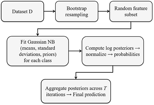
Figure 1. Workflow of RandomGaussianNB.

The following section formalizes its posterior-averaging properties and derives the generalization bound.

3.2 Theoretical properties of PAV-GNB

The posterior averaging Gaussian naive Bayes (PAV-GNB) ensemble aggregates the posterior probabilities from T independently randomized GNB classifiers trained on bootstrap samples and feature-subset draws.

Let P_t(C_k|x) denote the posterior for class C_k from the t- th model, and define the ensemble posterior

$\begin{array}{ll}{\bar{P}}_T(C_k|\text{x})=\frac{1}{T}{{\displaystyle \sum }}_{t=1}^T{P}_t(C_k|\text{x}).& (11)\end{array}$

Expectations and variances below are taken over bootstrap and feature randomization.

3.2.1 Consistency and variance

Under correct model specification and regularity of the plug-in estimators, each P_t(C_k|x) is consistent for the true posterior $p^{*}(C_k|\text{x})$; hence ${\bar{P}}_T$ is also consistent as n → ∞ (fixed T). Assuming equal marginal variance σ²(x) and average pairwise correlation ρ(x) across {P_t},

$\begin{array}{ll}Var\left[{\bar{P}}_T(C_k|\text{x})\right]=\frac{{\sigma }^2(\text{x})}{T}(1+\rho (\text{x})(T-1)).& (12)\end{array}$

Smaller overlap among D^(t) and F^(t) decreases ρ(x), yielding near−1/T variance reduction.

3.2.2 Quadratic-loss aggregation

For the Brier score (Brier, 1950; Geman et al., 1992; Breiman, 1996), the population minimizer is p^*(·|x). Among convex mixtures of {P_t}, the optimal weights depend on the error covariance; equal weights are optimal under exchangeability with equal variance and covariance, making simple averaging a stable, statistically efficient rule when base learners are approximately homogeneous and weakly correlated.

3.2.3 Margin-based generalization bound

Let the Bayes margin be $\gamma (\text{X})=p^{*}(Y\mid X)-{max}_{k\ne Y}{p}^{*}(C_k\mid \text{X})>0$. Suppose E[P_t(Y|X)]=p^*(Y|X) + b(X) and $Var\left[P_t(Y|\text{X})\right]={\sigma }^2(\text{X})$ with average pairwise correlation ρ(X). Then, for[u]₊ = max(u, 0),

$\begin{array}{ll}Pr\left[\widehat{C}(\text{X})\ne Y\right]\le \frac{{\sigma }^2(\text{X})\left\{1+\rho (\text{X})(T-1)\right\}}{T{\displaystyle {\left[\frac{\gamma (\text{X})}{2}-|b(\text{X})|\right]}_{+}^2}},& (13)\end{array}$

where $\widehat{C}(\text{X})=arg{max}_k{\bar{P}}_T(C_k|\text{X})$. The bound decays with larger T and smaller ρ, and tightens with larger margin and smaller bias.

A proof sketch for (12) and (13) is provided in Appendix A, detailing the equicorrelation calculation and the Cantelli step used in the margin-based bound.

3.3 RandomGaussianNB simulation design and dataset generation

Synthetic datasets are generated to systematically control key characteristics, including sample size n, number of features p, number of classes K, and correlation structures among features. Each dataset D in (14) consists of feature vectors x_i paired with corresponding class labels y_i:

$\begin{array}{ll}D={\left\{({\text{x}}_i,y_i)\right\}}_{i=1}^n,{\text{x}}_i\in {ℝ}^p,y_i\in \left\{0,1,...,K-1\right\}.& (14)\end{array}$

Each x_i for class k is sampled from a class-specific multivariate Gaussian distribution:

$\begin{array}{ll}{\text{x}}_i|(y_i=k)~N({\mu }_k,{\Sigma }_k),k=0,1,...,K-1,& (15)\end{array}$

with class-specific mean vectors μ_k and covariance matrices Σ_k.

Class overlap is regulated by adjusting μ_k and Σ_k. Separability is characterized using Mahalanobis distances between class means and controlled correlation parameters. Following Schober et al. (2018), correlation thresholds are interpreted as minimal (ρ = 0.1), moderate (ρ = 0.5), and strong (ρ = 0.9) associations, while the identity structure (ρ = 0) reflects independence. The systematically defined scenarios are summarized in Table 1.

Table 1

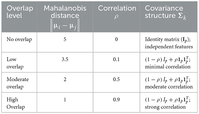
Table 1. Summary of class overlap levels and corresponding covariance structures.

3.4 Computational environment

All benchmarking experiments are conducted in a standardized computing environment to ensure reproducibility:

• Processor: Intel(R) Core(TM) i9-13980HX CPU, 2.20 GHz, 24 cores (32 logical processors)

• RAM: 64 GB

• Operating System: Microsoft Windows 11 Pro (Version 10.0.26100)

• R Version: 4.4.0

Parallel computation is implemented using the parallel (R Core Team, 2025) and foreach (Weston and Microsoft Corporation, 2022b) packages, enabling performance evaluation across different core settings (1, 2, 4, 8, 16, and 24 cores).

3.5 Benchmarking procedure

A comprehensive benchmarking protocol was designed to evaluate the runtime, scalability, and stability of the proposed PAV-GNB classifier. Experimental scenarios of varying complexity ensure broad coverage of practical conditions and reproducibility. Each scenario was independently repeated R = 10 times. Statistical differences were assessed by two-way ANOVA (α = 0.05) followed by Tukey's HSD post-hoc tests (Tukey, 1949).

3.5.1 Baseline experiments

Baseline experiments established reference performance under controlled conditions. Simulations used a fixed dataset size n = 1,000, dimensionality p = 50, three-class classification K = 3, feature fraction f = 0.25, number of iterations T = 100, and single-core computation (c = 1). Four class-overlap levels—no overlap (||μ_i − μ_j|| ≈ 5, ρ = 0), low overlap (≈ 3.5, ρ = 0.1), moderate overlap (≈ 2, ρ = 0.5), and high overlap (≈ 1, ρ = 0.9)— quantified the influence of data separability on accuracy and runtime.

3.5.2 Scalability analysis

To examine efficiency gains from parallel computation, moderate complexity parameters (n = 5000, p = 100, K = 3, f = 0.25, T = 100, ρ = 0.5) were retained while varying CPU cores c ∈ {1, 2, 4, 8, 16}. This analysis quantified runtime reduction and scalability efficiency E_s under increasing parallel resources.

3.5.3 Dimensionality and sample size stress test

Robustness under high-dimensional and large-sample conditions was assessed by systematically increasing dataset size n ∈ {500, 1000, 5000, 10, 000, 20, 000, 50, 000, 100, 000} and dimensionality p ∈ {10, 50, 100, 500, 1000, 2000}, while holding K = 3, f = 0.25, c = 4, T = 100, ρ = 0.5. These experiments probed computational feasibility from small to extremely large analytic scales.

3.5.4 Feature fraction sensitivity analysis

The effect of randomized feature selection was investigated by varying the feature fraction $f\in \{\sqrt{p}/p,1/10,1/5,1/4,1/3,1/2,1\},$ keeping other parameters fixed (n = 5000, p = 100, K = 3, c = 4, T = 100, ρ = 0.5). This clarified how subsampling proportions influence accuracy and runtime.

3.5.5 High complexity and multiclass performance

Classifier effectiveness under realistic large-scale conditions was evaluated with n = 100, 000, p = 1000, c = 8, f = 0.25), and class counts K ∈ {2, 3, 5, 10}. Experiments were conducted under moderate (ρ = 0.5) and high (ρ = 0.9) overlap to test robustness against severe class correlation.

3.5.6 Iterations and stability analysis

Finally, predictive stability was examined by varying the number of bootstrap iterations T = {10, 50, 100, 300, 500} while maintaining moderate complexity settings (n = 5000, p = 100, K = 3, c = 4, f = 0.25, ρ = 0.5). This assessed consistency of accuracy and runtime across repeated resampling.

3.6 Performance evaluation criteria

Three complementary metrics are used to assess computational efficiency and predictive performance:

(1) Computational Runtime (seconds): The mean total time for training and prediction across R independent repetitions is defined in (16):

$\begin{array}{ll}\text{Runtime}=\frac{1}{R}{{\displaystyle \sum }}_{r=1}^R(T_{\text{train},r}+T_{\text{predict},r}),& (16)\end{array}$

where T_{train, r} and T_{predict, r} denote the training and prediction times of the r-th run.

(2) Scalability Efficiency (E_S): Parallel-processing gains are quantified using (17) (Schryen, 2022):

$\begin{array}{ll}{\text{E}}_S=\frac{T_1}{c{T}_c},& (17)\end{array}$

where T₁ is the single-core runtime, T_c is runtime using c cores, and larger values indicate better parallel efficiency.

(3) Predictive Accuracy: Classification accuracy is computed as (18) (Powers, 2011; Kummaraka and Srisuradetchai, 2025):

$\begin{array}{ll}\text{Accuracy}=\frac{1}{n}{{\displaystyle \sum }}_{i=1}^{n}I\left({\widehat{y}}_i=y_i\right),& (18)\end{array}$

where ŷ_i is the predicted class, the true class, and I(·) an indicator function.

4 Experimental results

4.1 Baseline performance evaluation

Table 2 and Figure 2 summarize the baseline experiments assessing runtime and accuracy across four levels of class overlap: none, low, moderate, and high. Mean runtime remained stable as overlap increased, ranging from 7.769 s to 7.79 s. A Tukey HSD test confirmed no significant differences among these scenarios (p-value = 0.195), indicating that runtime was largely unaffected by class separability. Minor outliers observed in Figure 2 reflect normal variability from random initialization or hardware fluctuations rather than methodological effects.

Table 2

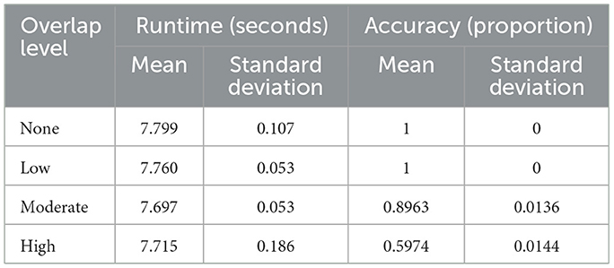
Table 2. Summary of baseline experiment results.

Figure 2

Figure 2. Baseline experiments: runtime (Left) and accuracy (Right) across class overlap scenarios.

Accuracy, in contrast, was strongly influenced by overlap. Perfect classification (mean = 1.0) was achieved when classes were well-separated (none or low overlap). Accuracy declined to 0.896 (SD = 0.014) under moderate overlap and dropped further to 0.598 (SD = 0.014) when classes substantially intersected. These results highlight that while computational cost is stable, prediction reliability decreases sharply as class distributions become less distinct, underscoring the challenge of learning in highly overlapping settings.

4.2 Scalability analysis

Scalability experiments evaluate how computational runtime and predictive accuracy vary with the number of CPU cores. Figure 3 (left) shows a sharp runtime reduction as parallelization increases, falling from a single-core mean of 15.20 s to 8.03 s (two cores), 5.04 s (four cores), and a minimum of 4.47 s at eight cores (see Table 3). A slight rise to 5.55 s at sixteen cores suggests diminishing returns or overhead from heavy parallel execution. Two-way ANOVA confirms significant runtime differences across core settings (F value = 486.1, p-value < 0.0001), while Tukey tests find no significant gap between four and eight cores (p-value = 0.295) or between four and sixteen cores (p-value = 0.378).

Figure 3

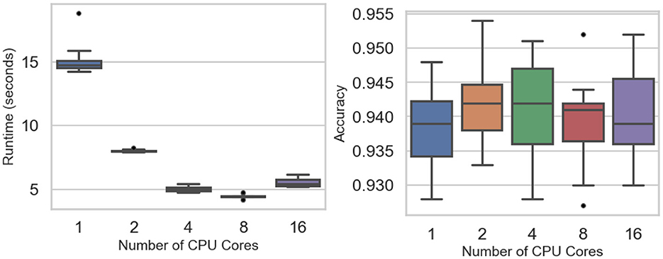
Figure 3. Scalability experiments: runtime (Left) and accuracy (Right) across the number of CPU cores.

Table 3

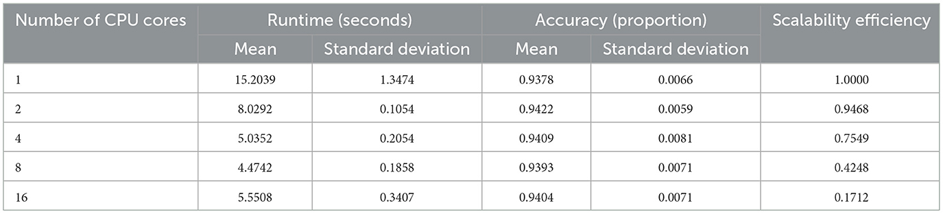
Table 3. Summary of scalability analysis.

Classification accuracy remains stable across all levels of parallelism (Figure 3, right), fluctuating narrowly between 0.938 and 0.942 (Table 3). The F-test (p-value = 0.915) indicates no significant accuracy difference among core counts. Scalability efficiency, E_s = T₁/(cT_c), declines from 0.95 (two cores) to 0.75 (four cores), 0.42 (eight cores), and 0.17 (sixteen cores), confirming that parallel speedup plateaus as core usage grows.

These findings indicate that speedup improves substantially up to eight cores, beyond which performance gains taper due to synchronization overhead and data-distribution costs, consistent with typical behavior in ensemble parallelization.

4.3 Dimensionality and sample size stress test

4.3.1 Impact of dimensionality on classifier performance

Figure 4 and Table 4 summarize how feature dimensionality influences runtime and accuracy. Computational cost rises sharply with higher dimensions: mean runtime stays below 10 s for 10–100 features but climbs to roughly 41 s at 500, 87 s at 1,000, and 160 s at 2,000 features. Two-way ANOVA confirms significant runtime differences (F value = 2,418, p-value < 0.0001). Tukey post-hoc tests show no significant gap between 10 and 50 features (p-value = 0.475) or between 50 and 100 (p-value = 0.202), but all larger jumps are significant, reflecting the quadratic growth in matrix operations.

Figure 4

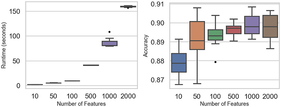
Figure 4. Dimensionality experiments: runtime (Left) and accuracy (Right) across the number of features.

Table 4

Table 4. Summary of dimensionality performance.

Despite these steep runtime increases, classification accuracy remains stable across all dimensional settings. Mean accuracy fluctuates only slightly—from 0.879 at 10 features to about 0.899 at 1,000 and 0.897 at 2,000—differences that are not statistically significant (F value = 0.562, p-value = 0.69). These results demonstrate that while computational demands scale rapidly with dimensionality, the predictive performance of the PAV-GNB classifier is largely unaffected, underscoring its robustness for high-dimensional data.

4.3.2 Sample size stress test

Figure 5 and Table 5 summarize the classifier's computational performance and accuracy across sample sizes from n = 500 to n = 200,000. Runtime scales predictably with dataset size: it remains below 5 s for n ≤ 5,000, rises to about 10 s at n = 20,000, and reaches 27 s, 53 s, and 107 s for n = 50,000, 100,000, and 200,000, respectively. ANOVA confirms a strong effect of sample size on runtime (F-value = 1.05 × 10⁵, p-value < 0.0001), with Tukey tests showing significant pairwise differences at nearly all adjacent sizes except between 500 and 1,000 observations (p-value = 0.571).

Figure 5

Figure 5. Sample size experiments: runtime (Left) and accuracy (Right) across the sample sizes.

Table 5

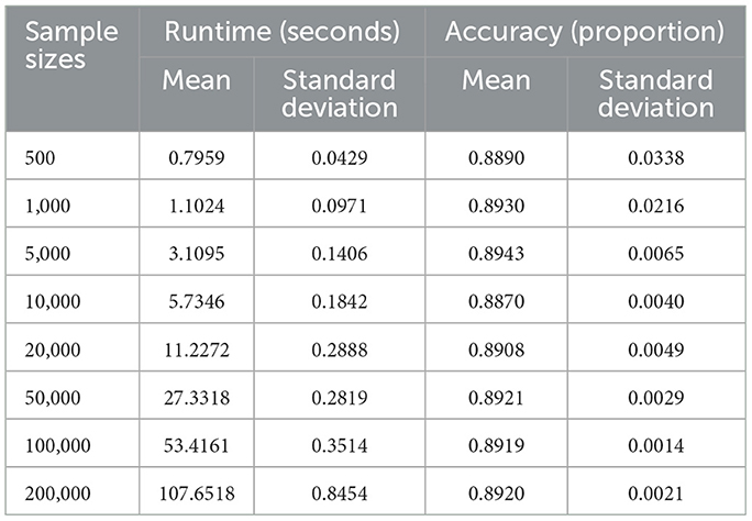
Table 5. Summary of sample sizes stress test.

4.4 Feature fraction analysis

The influence of feature subsampling on runtime and predictive accuracy is summarized in Table 6 and visualized in Figure 6. Runtime rises steadily as the fraction of utilized features increases. When small subsets such as $\sqrt{p}$ or p/10 are selected, mean runtime remains below 3 s, whereas employing all features (p/p) drives the mean to roughly 17.7 s. ANOVA confirms significant differences among fractions (F-value = 1620.89, p-value < 0.0001), and Tukey's tests identify strong contrasts between extreme settings (e.g., p vs. p/10, p/2 vs. p/10; both p-value < 0.0001). Only the comparison between $\sqrt{p}$ and p/10 shows no significant gap (p-value = 0.9963).

Table 6

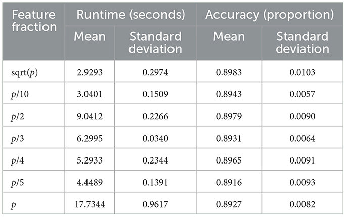
Table 6. Summary of feature fraction analysis.

Figure 6

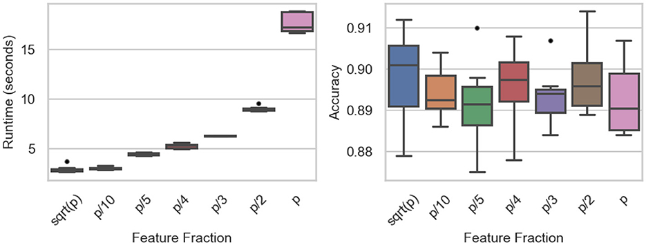
Figure 6. Feature fraction experiments: runtime (Left) and accuracy (Right) across the number of features.

Predictive accuracy, by contrast, remains stable across all feature fractions (Figure 6, right). Mean accuracy fluctuates slightly between 0.889 and 0.898, with ANOVA (F value = 0.5849, p-value = 0.742) and Tukey's HSD revealing no significant differences. These findings indicate that reducing the fraction of sampled features can markedly cut computation time without sacrificing classification performance, underscoring the method's efficiency under feature-randomized settings.

4.5 High complexity and multiclass performance analysis

This experiment examines classifier behavior under demanding conditions: 100,000 samples, 1,000 features, and a feature fraction of 0.25, with the number of classes varied (K∈{2, 3, 5, 10}) across moderate and high overlap. As presented in Figure 7 (left) and Table 7, runtime increases with class count, from about 601 s at two classes (moderate overlap) to roughly 783 s at ten classes, while high-overlap settings yield slightly shorter runtimes at each class level. Two-way ANOVA confirms significant runtime effects of both class number and overlap (F value = 116.40, p-value < 0.0001), with Tukey's tests highlighting strong contrasts between low- and high-complexity scenarios.

Figure 7

Figure 7. High complexity and multiclass analysis: runtime (Left) and accuracy (Right) across different numbers of classes and class overlap levels.

Table 7

Table 7. Summary of high complexity and multiclass analysis.

Predictive accuracy declines sharply as complexity rises. Mean accuracy reaches approximately 0.92 under the two-class moderate-overlap setting but falls to roughly 0.46 in the ten-class high-overlap case. ANOVA (F value = 10,304.17, p- value < 0.0001) and post-hoc comparisons verify significant accuracy reductions as overlap intensifies or the number of classes grows. These results underscore the computational and predictive challenges of simultaneous growth in class cardinality and overlap, providing a stringent stress test for the proposed PAV-GNB classifier.

4.6 Iterations and stability analysis

The influence of training iterations on computational cost and predictive reliability was examined under moderate settings (n = 10, 000, p = 100, K = 3, c = 4, f= 0.25, ρ = 0.5). Iteration counts were varied across five levels (T∈{10, 50, 100, 300, 500}). Figure 8 (left) and Table 8 show that runtime rises nearly linearly with additional iterations—from about 2 s at T = 10 to roughly 48 s at T = 500. ANOVA confirms significant differences among these levels (F = 643.81, p < 0.0001), reflecting the expected computational burden of repeated bootstrap–feature sampling.

Figure 8

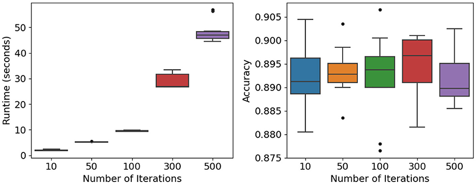
Figure 8. Iterations and stability analysis: runtime (Left) and accuracy (Right) across different numbers of training iterations.

Table 8

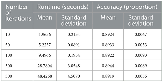
Table 8. Summary of iteration counts and stability analysis.

Despite this increase in runtime, predictive accuracy remains stable. As shown in Figure 8 (right) and Table 8, mean accuracy consistently falls within the 0.89–0.90 range, and ANOVA detects no significant variation across iteration counts (F value = 0.223, p-value = 0.924).

Conceptually, RandomGaussianNB parallels tree-based ensembles such as random forest or XGBoost (Chen and Guestrin, 2016) in using bootstrap and random subspaces for variance reduction, yet differs by aggregating probabilistic density estimates rather than split-based decisions. This preserves model interpretability while achieving comparable scalability.

5 Implementation and usage of the RandomGaussianNB package

5.1 Package overview

The RandomGaussianNB package provides a scalable and user-friendly implementation of the PAV-GNB classifier. It combines the efficiency of GNB with the robustness of bootstrap aggregation and randomized feature subsetting. The current version is maintained in a private GitHub repository; a public release and CRAN submission are planned following acceptance of this manuscript. This approach ensures future reproducibility, open access, and community support while allowing readers to cite the package as the canonical reference once it is publicly available.

5.2 Core functions and arguments

The main function, random_gaussian_nb(), trains an ensemble of GNB classifiers. Key arguments are:

• data: a data.frame or matrix of predictors and the response variable.

• response: the name of the response column (factor).

• n_iter: number of bootstrap iterations (default = 100).

• feature_fraction: proportion of predictors randomly selected at each iteration (default = 0.5).

• cores: number of parallel workers (default = 1).

An S3 predict() method supports both “class” (predicted label) and “prob” (posterior probability) outputs. The argument newdata allows application of the fitted model to new observations.

5.3 Workflow and example application

A typical workflow is illustrated using the PimaIndiansDiabetes dataset from the mlbench package (Leisch and Dimitriadou, 2024; Blake and Merz, 1998):

library(RandomGaussianNB)

library(mlbench)

# Load data

data(“PimaIndiansDiabetes”)

df <- PimaIndiansDiabetes

# Train-test split

set.seed(123)

n <- nrow(df)

train_idx <- sample(n, size = 0.7 * n)

train_df <- df[train_idx,]

test_df <- df[-train_idx,]

# Fit the PAV-GNB model

model <- random_gaussian_nb(

data = train_df,

response = “diabetes”,

n_iter = 100,

feature_fraction = 0.5,

cores = 2

)

# Predictions

probs <- predict(model,

test_df[, setdiff(names(test_df),“diabetes”)],

type = “prob”)

preds <- predict(model,

test_df[, setdiff(names(test_df),“diabetes”)],

type = “class”)

# Evaluate accuracy

mean(preds = = test_df$diabetes)

Using a 70/30 train–test split, the PAV-GNB classifier achieved an accuracy of 0.762, exceeding or matching the performance of several standard algorithms—classical GNB (0.758), k-nearest neighbors (k = 5; 0.753), support vector machine with radial kernel (0.758), random forest (0.745), decision tree (0.710), and a simple neural network (0.662) (Table 9). This experiment highlights the package's balance between simplicity, interpretability, and predictive strength relative to widely used classifiers.

Table 9

Table 9. Accuracy comparison of PAV-GNB with other standard classifiers on the PimaIndiansDiabetes dataset.

6 Conclusions

This study presented RandomGaussianNB, an open-source R package implementing the PAV-GNB algorithm—a scalable ensemble extension of GNB integrating bootstrap resampling, randomized feature subspaces, and posterior averaging. Theoretical analysis (Section 3.2) showed that posterior averaging minimizes quadratic risk, achieves mean-square optimality among convex combinations of base posteriors, and reduces variance under correlated features. The derived margin-based generalization bound links posterior variance to classification error, formalizing the ensemble's bias–variance balance.

Algorithmically (Section 3.1), PAV-GNB stabilizes GNB through ensemble randomization and parallel computation. The RandomGaussianNB package offers a reproducible S3 implementation and benchmarking pipeline for assessing accuracy, calibration, and scalability. Simulation studies (Sections 4.1–4.6) confirmed theoretical predictions—showing consistent accuracy, low variance, and stable calibration across diverse data conditions. Parallel execution achieved near-linear runtime gains, validating computational scalability.

A real-world test on the Pima Indians Diabetes dataset verified its reliability, matching or outperforming standard classifiers (classical GNB, k-NN, decision tree, random forest, SVM) with interpretability and efficiency. Future work will extend support to multi-modal data, advanced calibration, and cross-language use, reinforcing PAV-GNB as a statistically grounded and efficient framework for large-scale probabilistic classification.

Data availability statement

Publicly available datasets were analyzed in this study. This data can be found here: https://cran.r-project.org/package=mlbench.

Author contributions

PS: Conceptualization, Data curation, Formal analysis, Funding acquisition, Investigation, Methodology, Project administration, Resources, Software, Supervision, Validation, Visualization, Writing – original draft, Writing – review & editing.

Funding

The author(s) declare that no financial support was received for the research and/or publication of this article.

Acknowledgments

The author thanks the reviewers for their constructive comments and valuable suggestions, which helped improve the quality of this manuscript.

Conflict of interest

The author declares that the research was conducted in the absence of any commercial or financial relationships that could be construed as a potential conflict of interest.

Generative AI statement

The author(s) declare that no Gen AI was used in the creation of this manuscript.

Any alternative text (alt text) provided alongside figures in this article has been generated by Frontiers with the support of artificial intelligence and reasonable efforts have been made to ensure accuracy, including review by the authors wherever possible. If you identify any issues, please contact us.

Publisher's note

All claims expressed in this article are solely those of the authors and do not necessarily represent those of their affiliated organizations, or those of the publisher, the editors and the reviewers. Any product that may be evaluated in this article, or claim that may be made by its manufacturer, is not guaranteed or endorsed by the publisher.

Supplementary material

The Supplementary Material for this article can be found online at: https://www.frontiersin.org/articles/10.3389/fdata.2025.1706417/full#supplementary-material

References

Ara, A., and Louzada, F. (2022). Alpha-skew Gaussian Naive Bayes classifier. Int. J. Inform. Technol. Decis. Making 21, 441–462. doi: 10.1142/S0219622021500644

Crossref Full Text | Google Scholar

Askari, A., d'Aspremont, A., and El Ghaoui, L. (2020). “Naive feature selection: sparsity in Naive Bayes,” in Proceedings of the 23rd International Conference on Artificial Intelligence and Statistics (AISTATS 2020), Vol. 108 (Palermo: PMLR), 1813–1822.

Google Scholar

Barber, D. (2012). Bayesian Reasoning and Machine Learning. Cambridge: Cambridge University Press. doi: 10.1017/CBO9780511804779

Crossref Full Text | Google Scholar

Bhamre, N., Ekhande, P. P., and Pinsky, E. (2025). Enhancing naive Bayes algorithm with stable distributions for classification. Int. J. Cybernet. Inform. 14, 107–116. doi: 10.5121/ijci.2025.140207

Crossref Full Text | Google Scholar

Biau, G., and Scornet, E. (2016). A random forest guided tour. Test. 25, 197–227. doi: 10.1007/s11749-016-0481-7

Crossref Full Text | Google Scholar

Bishop, C. (2006). Pattern Recognition and Machine Learning. New York, NY: Springer.

Google Scholar

Blake, C. L., and Merz, C. J. (1998). UCI Repository of Machine Learning Databases. Irvine, CA: University of California, Department of Information and Computer Sciences.

Google Scholar

Boli, B. I. A.-D., and Wei, C. (2024). Bayesian classifier based on robust kernel density estimation and Harris hawks optimisation. Int. J. Internet Distrib. Syst. 6, 1–23. doi: 10.4236/ijids.2024.61001

Crossref Full Text | Google Scholar

Boulle, F. (2007). Compression-based averaging of selective Naive Bayes classifiers. J. Mach. Learn. Res. 8, 165–185.

Google Scholar

Breiman, L. (1996). Bagging predictors. Mach. Learn. 24, 123–140. doi: 10.1023/A:1018054314350

Crossref Full Text | Google Scholar

Breiman, L. (2001). Random forests. Mach. Learn. 45, 5–32. doi: 10.1023/A:1010933404324

Crossref Full Text | Google Scholar

Brier, G. W. (1950). Verification of forecasts expressed in terms of probability. Mon. Weather Rev. 78, 1–3.2.

Google Scholar

Chen, T., and Guestrin, C. (2016). “XGBoost: a scalable tree boosting system,” in Proceedings of the 22nd ACM SIGKDD International Conference on Knowledge Discovery and Data Mining (KDD 2016), San Francisco, CA, USA (New York, NY: Association for Computing Machinery), 785–794. doi: 10.1145/2939672.2939785

Crossref Full Text | Google Scholar

Davidson, I. (2004). “An ensemble technique for stable learners with performance bounds,” in Proceedings of the AAAI Workshop on Bootstrapping Machine Learning, San Jose, CA, USA (Menlo Park, CA: AAAI Press), 330–335.

Google Scholar

DiCiccio, T. J., and Efron, B. (1996). Bootstrap confidence intervals. Stat. Sci. 11, 189–212. doi: 10.1214/ss/1032280214

Crossref Full Text | Google Scholar

Dietterich, T. G. (2000). “Ensemble methods in machine learning,” in Multiple Classifier Systems, Lecture Notes in Computer Science, eds. J. Kittler and F. Roli (Berlin; Heidelberg: Springer), 1–15. doi: 10.1007/3-540-45014-9_1

Crossref Full Text | Google Scholar

Dietterich, T. G., and Kong, E. B. (1995). Machine Learning Bias, Statistical Bias, and Statistical Variance of Decision Tree Algorithms. Tech. Rep. Oregon State University, Corvallis, OR.

Google Scholar

Domingos, P., and Pazzani, M. (1997). On the optimality of the simple Bayesian classifier under zero-one loss. Mach. Learn. 29, 103–130. doi: 10.1023/A:1007413511361

Crossref Full Text | Google Scholar

Efron, B., and Tibshirani, R. J. (1994). An Introduction to the Bootstrap. Boca Raton, FL: Chapman and Hall/CRC. doi: 10.1201/9780429246593

Crossref Full Text | Google Scholar

Elidan, G. (2012). Copula network classifiers (CNCs). “Proceedings of machine learning research,” in Proceedings of the 15th International Conference on Artificial Intelligence and Statistics (AISTATS 2012), Vol. 22, 346–354. Available online at: https://proceedings.mlr.press/v22/elidan12a/elidan12a.pdf (Accessed January 24, 2025).

Google Scholar

Freund, Y., and Schapire, R. E. (1997). A decision-theoretic generalization of on-line learning and an application to boosting. J. Comput. Syst. Sci. 55, 119–139. doi: 10.1006/jcss.1997.1504

Crossref Full Text | Google Scholar

Friedman, N., Geiger, D., and Goldszmidt, M. (1997). Bayesian network classifiers. Mach. Learn. 29, 131–163. doi: 10.1023/A:1007465528199

Crossref Full Text | Google Scholar

Geman, S., Bienenstock, E., and Doursat, R. (1992). Neural networks and the bias/variance dilemma. Neural Comput. 4, 1–58. doi: 10.1162/neco.1992.4.1.1

Crossref Full Text | Google Scholar

Guyon, I., and Elisseeff, A. (2003). An introduction to variable and feature selection. J. Mach. Learn. Res. 3, 1157–1182.

Google Scholar

Hall, M. A. (1999). Correlation-Based Feature Selection for Machine Learning (Ph.D. thesis). University of Waikato, Hamilton, New Zealand.

Google Scholar

Hand, D. J., and Yu, K. (2001). Idiot's Bayes—Not so stupid after all? Int. Stat. Rev. 69, 385–398. doi: 10.1111/j.1751-5823.2001.tb00465.x

Crossref Full Text | Google Scholar

Ho, T. K. (1998). The random subspace method for constructing decision forests. IEEE Trans. Pattern Anal. Mach. Intell. 20, 832–844. doi: 10.1109/34.709601

Crossref Full Text | Google Scholar

Hochreiter, S., and Schmidhuber, J. (1997). Long short-term memory. Neural Comput. 9, 1735–1780. doi: 10.1162/neco.1997.9.8.1735

Crossref Full Text | Google Scholar

Jurafsky, D., and Martin, J. H. (2008). Speech and Language Processing, 2nd Edn. Upper Saddle River, NJ: Prentice Hall.

Google Scholar

Kamlangdee, P., and Srisuradetchai, P. (2025). Circular bootstrap on residuals for interval forecasting in K-NN regression: a case study on durian exports. Sci. Technol. Asia 30, 79–94.

Google Scholar

Kuhn, M. (2008). Building predictive models in R using the caret package. J. Stat. Softw. 28, 1–26. doi: 10.18637/jss.v028.i05

Crossref Full Text | Google Scholar

Kummaraka, U., and Srisuradetchai, P. (2025). Monte Carlo dropout neural networks for forecasting sinusoidal time series: performance evaluation and uncertainty quantification. Appl. Sci. 15:4363. doi: 10.3390/app15084363

Crossref Full Text | Google Scholar

LeCun, Y., Bottou, L., Bengio, Y., and Haffner, P. (1998). Gradient-based learning applied to document recognition. Proc. IEEE 86, 2278–2324. doi: 10.1109/5.726791

Crossref Full Text | Google Scholar

Leisch, F., and Dimitriadou, E. (2024). mlbench: Machine Learning Benchmark Problems. R package version 2.1-6. Available online at: https://CRAN.R-project.org/package=mlbench

Google Scholar

Li, J., Cheng, K., Wang, S., Morstatter, F., Trevino, R. T., Tang, J., et al. (2017). Feature selection: a data perspective. ACM Comput. Surv. 50:94. doi: 10.1145/3136625

Crossref Full Text | Google Scholar

Liapis, C. M., Karanikola, A., and Kotsiantis, S. B. (2023). A multivariate ensemble learning method for medium-term energy forecasting. Neural Comput. Appl. 35, 21479–21497. doi: 10.1007/s00521-023-08777-6

Crossref Full Text | Google Scholar

Liaw, A., and Wiener, M. (2002). Classification and regression by randomForest. R News 2, 18–22.

Google Scholar

Mahmud, M. S., Huang, J. Z., Salloum, S., Emara, T. Z., and Sadatdiynov, K. (2020). A survey of data partitioning and sampling methods to support big data analysis. Big Data Min. Anal. 3, 85–101. doi: 10.26599/BDMA.2019.9020015

Crossref Full Text | Google Scholar

McCallum, A., and Nigam, K. (1998). “A comparison of event models for naive Bayes text classification,” in Proceedings of the AAAI Conference on Artificial Intelligence (AAAI-98), Madison, WI, USA (Menlo Park, CA: AAAI Press), 41–48.

Google Scholar

Meyer, D., Dimitriadou, E., Hornik, K., Weingessel, A., and Leisch, F. (2024). e1071: Misc Functions of the Department of Statistics, Probability Theory Group, TU Wien. R package version 1.7-16. Available online at: https://CRAN.R-project.org/package=e1071

Google Scholar

Mitchell, T. (1997). Machine Learning. New York, NY: McGraw-Hill.

Google Scholar

Murphy, K. P. (2012). Machine Learning: A Probabilistic Perspective. Cambridge, MA: MIT Press.

Google Scholar

Panichkitkosolkul, W., and Srisuradetchai, P. (2022). Bootstrap confidence intervals for the parameter of zero-truncated Poisson-Ishita distribution. Thailand Statist. 20, 918–927.

Google Scholar

Pearl, J. (1988). Probabilistic Reasoning in Intelligent Systems: Networks of Plausible Inference. San Mateo, CA: Morgan Kaufmann. doi: 10.1016/B978-0-08-051489-5.50008-4

Crossref Full Text | Google Scholar

Pedregosa, F., Varoquaux, G., Gramfort, A., Michel, V., Thirion, B., Grisel, O., et al. (2011). Scikit-learn: machine learning in Python. J. Mach. Learn. Res. 12, 2825–2830. doi: 10.5555/1953048.2078195

Crossref Full Text | Google Scholar

Phatcharathada, B., and Srisuradetchai, P. (2025). Randomized feature and bootstrapped naive Bayes classification. Appl. Syst. Innov. 8:94. doi: 10.3390/asi8040094

Crossref Full Text | Google Scholar

Polikar, R. (2006). Ensemble based systems in decision making. IEEE Circuits Syst. Mag. 6, 21–45. doi: 10.1109/MCAS.2006.1688199

Crossref Full Text | Google Scholar

Powers, D. M. W. (2011). Evaluation: from precision, recall and F-measure to ROC, informedness, markedness and correlation. J. Mach. Learn. Technol. 2, 37–63.

Google Scholar

R Core Team (2025). R: A Language and Environment for Statistical Computing. Vienna, Austria: R Foundation for Statistical Computing.

Google Scholar

Ratanamahatana, C., and Gunopulos, D. (2003). Feature selection for the naive Bayesian classifier using decision trees. Appl. Artif. Intell. 17, 475–487. doi: 10.1080/713827175

Crossref Full Text | Google Scholar

Rennie, J. D., Shih, L., Teevan, J., and Karger, D. (2003). “Tackling the poor assumptions of naive Bayes text classifiers,” in Proceedings of the 20th International Conference on Machine Learning (ICML 2003), Washington, DC, USA (Menlo Park, CA: AAAI Press), 616–623.

Google Scholar

Rish, I. (2001). “An empirical study of the naive Bayes classifier,” in IJCAI Workshop on Empirical Methods in Artificial Intelligence (Seattle, WA: IJCAI Organization), 41–46.

Google Scholar

Sagi, O., and Rokach, L. (2018). Ensemble learning: a survey. WIREs Data Min. Knowl. Discov. 8:e1249. doi: 10.1002/widm.1249

Crossref Full Text | Google Scholar

Schapire, R. E. (2003). “The boosting approach to machine learning: an overview,” in Nonlinear Estimation and Classification (New York, NY: Springer), 149–171. doi: 10.1007/978-0-387-21579-2_9

Crossref Full Text | Google Scholar

Schober, P., Boer, C., and Schwarte, L. A. (2018). Correlation coefficients: appropriate use and interpretation. Anesth. Analg. 126, 1763–1768. doi: 10.1213/ANE.0000000000002864

PubMed Abstract | Crossref Full Text | Google Scholar

Schryen, G. (2022). Speedup and efficiency of computational parallelization: a unifying approach and asymptotic analysis. arXiv preprint arXiv:2212.11223. doi: 10.2139/ssrn.4327867

Crossref Full Text | Google Scholar

Shawe-Taylor, J., and Cristianini, N. (2004). Kernel Methods for Pattern Analysis. Cambridge: Cambridge University Press. doi: 10.1017/CBO9780511809682

Crossref Full Text | Google Scholar

Soria, D., Garibaldi, J. M., Ambrogi, F., Biganzoli, E. M., and Ellis, I. O. (2011). A ‘non-parametric' version of the Naive Bayes classifier. Knowl. -Based Syst. 24, 775–784. doi: 10.1016/j.knosys.2011.02.014

Crossref Full Text | Google Scholar

Sriprasert, S., and Srisuradetchai, P. (2025). Multi-K KNN regression with bootstrap aggregation: accurate predictions and alternative prediction intervals. Edelweiss Appl. Sci. Technol. 9, 2750–2764. doi: 10.55214/25768484.v9i5.7589

Crossref Full Text | Google Scholar

Tantalaki, N., Souravlas, S., and Roumeliotis, M. (2020). A review on big data real-time stream processing and its scheduling techniques. Int. J. Parallel, Emergent Distrib. Syst. 35, 571–601. doi: 10.1080/17445760.2019.1585848

Crossref Full Text | Google Scholar

Tukey, J. W. (1949). Comparing individual means in the analysis of variance. Biometrics 5, 99–114. doi: 10.2307/3001913

PubMed Abstract | Crossref Full Text | Google Scholar

Urbanowicz, R. J., Meeker, M., La Cava, W., Olson, R. S., and Moore, J. H. (2018). Relief-based feature selection: introduction and review. J. Biomed. Inform. 85, 189–203. doi: 10.1016/j.jbi.2018.07.014

PubMed Abstract | Crossref Full Text | Google Scholar

Wang, B., Sun, Y., Zhang, T., Sugi, T., and Wang, X. (2020). Bayesian classifier with multivariate distribution based on D-vine copula model for awake/drowsiness interpretation during power nap. Biomed. Signal Process. Control 56:101686. doi: 10.1016/j.bspc.2019.101686

Crossref Full Text | Google Scholar

Wang, Q., Garrity, G. M., Tiedje, J. M., and Cole, J. R. (2007). Naive Bayesian classifier for rapid assignment of rRNA sequences into the new bacterial taxonomy. Appl. Environ. Microbiol. 73, 5261–5267. doi: 10.1128/AEM.00062-07

PubMed Abstract | Crossref Full Text | Google Scholar

Wang, Y., Zhang, W., Li, X., Wang, A., Wu, T., and Bao, Y. (2020). “Monthly load forecasting based on an ARIMA-BP model: a case study on Shaoxing city,” in 12th IEEE PES Asia-Pacific Power and Energy Engineering Conf. (APPEEC) (Nanjing: IEEE), 1–6. doi: 10.1109/APPEEC48164.2020.9220521

Crossref Full Text | Google Scholar

Weston, S. (2022a). doParallel: Foreach Parallel Adaptor for the ‘Parallel' Package. R package version 1.0.17. Microsoft Corporation, Redmond, WA.

Google Scholar

Weston, S. (2022b). foreach: Provides Foreach Looping Construct. R package version 1.5.2. Microsoft Corporation, Redmond, WA.

Google Scholar

Zhang, H. (2004). “The optimality of naive Bayes,” in Proceedings of the 17th International Florida Artificial Intelligence Research Society Conference (FLAIRS 2004), Miami Beach, FL, USA (Menlo Park, CA: AAAI Press), 562–567.

Google Scholar

Zhang, T. (2004). “Solving large scale linear prediction problems using stochastic gradient descent algorithms,” in Proceedings of the 21st International Conference on Machine Learning (ICML'04), Banff, Alberta, Canada (New York, NY: Association for Computing Machinery), 1–10. doi: 10.1145/1015330.1015332

Crossref Full Text | Google Scholar

Zhou, Z.-H. (2012). Ensemble Methods: Foundations and Algorithms. Boca Raton, FL: Chapman and Hall/CRC. doi: 10.1201/b12207

Crossref Full Text | Google Scholar