Opportunistic mobile air quality mapping using sensors on postal service vehicles: from point clouds to actionable insights

This study aimed to examine the validity of a mobile air quality sensor fleet in improving pollution exposure assessments in urban areas. The scope of this study involved experimental setup (sensor validation and calibration), evaluation of spatiotemporal data coverage, and analysis of the representativity of the collected mobile data. The results showed that indicative sensor data quality can be achieved after NO₂ co-location calibration, although particulate matter exhibited unsatisfactory performance. An extensive mobile air quality dataset was collected in Antwerp city between February and September 2021, covering 945 km of road by a total of ∼7.9 million data points, yielding an average segment coverage of 1,050 measurements per street segment (median = 62). The collected mobile data were made available in an open data repository. From the introduced area (%) and street segment (n) coverage, we can conclude that opportunistic data collection using service fleet vehicles (e.g., postal vans) is an efficient approach for covering a wide spatial area and collecting many repeated runs (∼200 measurements/segment/month). Monthly maps showed recurring pollution gradients with hotspot locations both at the suspected (e.g., busy traffic arteries) and unexpected locations, with observed increments greatly exceeding the observed inter-sensor uncertainty. The existing air quality monitoring network (five air quality monitoring stations) properly reflected the observed NO₂ exposure range (temporal variability), which was documented by the sensor fleet in Antwerp. The spatial exposure variability was improved significantly by the sensor fleet with 59% of the total street length covered after 1 month of mobile deployment (February–March). We required ∼45 repeated passages (31 after post-processing) to derive representative long-term NO₂ exposure data from this opportunistic dataset. Our findings suggested that opportunistic data collection using sensors on service fleet vehicles is a valid approach for pollution exposure assessments, through proper validation and calibration strategy. Temporary deployment of mobile sensors was a valuable approach for cities with a less extensive (or lack) air quality monitoring network or those who want a more fine-grained air quality mapping.

GRAPHICAL ABSTRACT

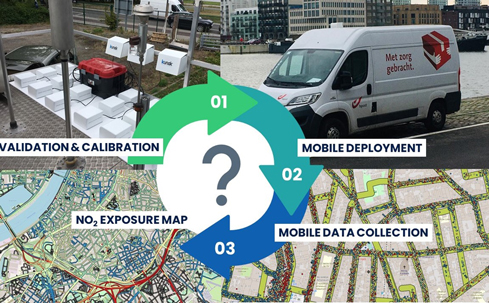
GRAPHICAL ABSTRACT

1. Introduction

Although urbanization and densification are considered sustainable solutions to optimize the supply chain of goods and services to an ever-growing population, they have a negative impact on the environmental quality and health of citizens. Major cities often comprise densely populated residential areas near busy road networks, harbors, and/or industrial sites, resulting in local hotspots of water, air, and soil pollution, noise, and heat stress. State and extent mapping is challenging because existing monitoring networks are sparsely sited and environmental stressors often consist of local hotspots, exhibiting steep gradients across space and time.

The recent advances in the Internet of Things (IoT) and sensor technology have resulted in smaller and more affordable environmental sensing solutions; hence, regulatory monitoring networks are complemented with mobile or stationary monitoring solutions enabling a higher coverage of spatiotemporal monitoring and more accurate exposure assessments. Although these low-cost sensing solutions provide a wide range of applications, they typically have a lower accuracy compared to that of the regulatory monitoring networks (1, 2). Moreover, they are more sensitive to meteorological conditions (e.g., temperature and humidity) or other pollutants and exhibit sensor drift over time (1–7). Executing proper calibration and validation of the applied sensor application is, therefore, vital to ensuring reliable and meaningful results (8–15). Although complementary monitoring through stationary sensor solutions has been successfully showcased in dedicated air quality (AQ) applications that are confined in time and space [e.g., to quantify the impact of traffic interventions (10)], city-wide and long-term monitoring requires an unrealistically high amount of sensors and associated maintenance and calibration efforts. Therefore, recent research has focused on distant or network-based calibration approaches, not requiring co-location calibrations next to an air quality monitoring station (AQMS), while ensuring data quality performance over time (9, 14, 16–18).

Mobile monitoring applications, where instruments are mounted on a mobile platform (person, bicycle, car, tram) moving around the city to improve the spatiotemporal resolution of air quality data, provide an alternative solution to dense stationary sensor networks by generating city-wide pollutant exposure maps (19–26). This methodology involves a range of applications, e.g., air quality mapping, personal exposure assessments, hotspot detection, evaluation of policy measures, and validation of pollutant dispersion models. Today, the main focus of mobile sensing applications is on short-term personal exposure assessments or the derivation of long-term exposure maps. A wide range of mobile applications has been explored in the field, from low-cost to high-end instruments, big data to small-scale field campaigns, and opportunistic to dedicated monitoring routes. Mobile sensing has been deployed on service fleet vehicles, e.g., garbage trucks in Cambridge, MA (USA) (20), and trams and buses in Lausanne and Zurich (Switzerland) (27), whereas monitoring instruments have been deployed on cars (19, 28), bicycles (26, 29–33), and city wardens (34). The collected mobile data provide valuable in situ data on exposure levels experienced by people around the city. Nevertheless, these data are still confined in time and space, and proper processing is required to derive representative (location-averaged) exposure maps (24, 35, 36).

This study aimed to examine the validity of a mobile IoT sensor fleet in collecting fine-grained air quality data to gain more insight into urban air pollution exposure. We performed (1) validation and calibration of a commercial IoT sensor solution; (2) in situ deployments on top of 17 postal service vehicles in Antwerp, Belgium; (3) evaluation of this opportunistic sampling strategy in terms of spatiotemporal coverage and representativity; and (4) evaluation of the sensor performance over time.

2. Materials and methods

2.1. Study area

Antwerp, a large (529,417 inhabitants) and densely populated (2,591 inhabitants/km²) city in northern Belgium (51° 13′ 17″ N, 4° 23′ 49.99″ E) was chosen as the study area. The city center is surrounded by a busy ring road and bounded by Europe’s second-largest port (viz., the Port of Antwerp). The combination of dense population, busy traffic, harbors, and industrial activities has drawn air quality concerns in the past, leading to many dedicated air quality studies in both mobile (30, 32, 37) and fixed (37–42) monitoring or modeling (43–48) studies.

2.2. Mobile sensor solution

In the 2021 BelAir project, Interuniversity Microelectronics Centre (IMEC) (BE), IMEC the Netherlands (NL), and the postal service of Belgium (Bpost) collaborated in testing and deploying 20 mobile IoT sensor systems in Antwerp city. We selected the Kunak® Air Mobile (Kunak Technologies SL, Spain) sensor systems comprising an optical sensor for particulate matter (PM; OPC-N3, AlphaSense), electrochemical gas sensors for nitrogen dioxide (NO₂; NO2-B43F, AlphaSense) and ozone (O₃; OX-B431, AlphaSense), global positioning system (GPS), and long-term evolution machine-type (LTE-M) communication and built in a dedicated LABAQUA housing to avoid turbulence over the sensors (Figure 1). Although mobile sensing applications can be employed in various mobile platforms (e.g., pedestrians, bicycles, dedicated cars, garbage trucks, public transport), we opted for postal service fleet vehicles because they operate every day (except for Sunday) between ∼5 and 18 h and deliver at “every doorstep,” providing good coverage of city spatial monitoring. Further specifications of the Kunak® Air Mobile are listed in Table 1.

FIGURE 1

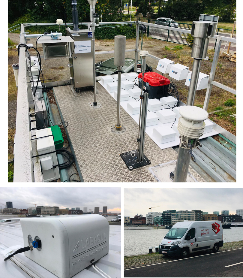
Figure 1. Kunak® Air Mobile sensor systems co-located at the R817 AQMS; three in fixed shields, 17 in mobile enclosure (upper), details of the Kunak® Air Mobile sensor system (lower left), and rooftop deployment on a postal van in Antwerp (lower right).

TABLE 1

Table 1. Sensor system specifications of the Kunak® Air Mobile.

2.3. Calibration and validation

In January 2021, 20 sensor systems were co-located at an urban background AQMS in Antwerp (R817; Figure 1) to perform sensor validation (correlation, accuracy, precision) and an additional local calibration to further optimize the accuracy (10, 49–51). In addition to the device property algorithm compensating for temperature, relative humidity (RH), and other sensor confounders, a cloud calibration tool was provided in the Kunak Air Cloud platform (https://www.kunakcloud.com) consisting of a mass factor (linear slope) calibration tool for PM (REF = slope × sensor) and baseline (∼0 ppb) and span (30–40 ppb) calibration tool for NO₂. Calibration was performed sequentially in batches of five sensors (in fixed shields), 1-week co-location data were used for training (fitting regression slopes/exhibition of zero/span concentrations), and another 1-week co-location data were used to evaluate the performance of the sensors after calibration (2 weeks/sensor batch). After calibration, the sensor batches were deployed sequentially on the postal vans. Three sensor boxes (IDs 18, 19, and 20) remained co-located at the AQMS to evaluate their performance over time, and 17 sensor boxes were deployed on postal vans.

Performance evaluation was based on accuracy [root mean squared error (RMSE) and mean absolute error (MAE)] and correlation [coefficient of determination (R²)], statistics between the sensor data (raw vs. calibrated), and the co-located reference measurements (52–54). In addition, we evaluated the uncertainty at the limit or target values using the non-parametric approach proposed by the Flanders Environmental Agency, that is, ∼50 µg m⁻³ for PM₁₀, 30 µg m⁻³ for PM_2.5, and 40 µg m⁻³ for NO₂. From the actual sensor measurements, this expanded uncertainty (U_exp; %) was quantified experimentally as the 95% MAE of measurements within the 10% range of the regulatory limit/target concentration. According to a color code developed during the VAQUUMs project (53), the tested sensors correspond to the supplementary class when the % difference from the equivalent method (expanded uncertainty) is <50% for PM and <25% for NO₂ (Supplementary Appendix S3). These values (%) were also within the data quality objectives (DQO) for indicative measurements as defined in AQ Directive 2008/50/EC (and corresponding to the DQO required for Class 1 sensor systems for NO₂ in CEN/TS 17660-1:2021); however, these were not tested following the protocol (test location, test period, and seasons).

Three sensor systems remained co-located next to the AQMS to evaluate their performance over time. With this, we calculated the performance statistics from the beginning (March) to the end (September) of the monitoring campaign, evaluated the potential sensor drift expressed as the sensor-to-reference (sensor/REF) ratio over time, and investigated the potential impacts from seasonality. The between-sensor uncertainty (BSU) (54) was calculated to evaluate the comparability between the sensors. This metric is important and must be considered when a sensor network is deployed. The low BSU could ensure that all the devices installed in the field have the same performance under different conditions. Thus, using the three devices installed in the AQMS could evaluate the drift of the remaining devices in the field.

2.4. Mobile deployments

After calibration, the sensor batches (each with five sensors) were deployed sequentially on the postal vans between January and March 2021. The sensor units were mounted in front of the roof, at the opposite side of the car exhaust, to avoid self-sampling as much as possible (Figure 1). Postal routes can be considered opportunistic if vans deliver packages to varying postal addresses. These vans were operational from Monday to Saturday, between ∼5 and 18 h, and were stationary and parked outside at the postal depot (51° 14′ 16.75″ N, 4° 24′ 57.97″ E) overnight on Sunday. This routine can be observed from the collected driving speeds of the 17 sensor systems as provided in Supplementary Appendix S1. We configured the monitoring resolution of the sensors to 10 s during service times (when mobile) and 5 min overnight (when parked) to avoid battery drainage of the sensor systems.

2.5. Data processing

2.5.1. Data cleaning and exploration

The collected mobile data consisted of a timestamp; a device ID; latitude/longitude coordinates (°); measured concentrations of PM₁, PM_2.5, PM₁₀ (µg m⁻³), and NO₂ (ppb); external temperature (°C); RH (%); and driving speed (km h⁻¹). Data cleaning was performed to exclude data points containing only pollutant concentrations or geographical data (incomplete data points) and notable outliers. Subsequently, we selected our study area (51.18517117° < Latitude < 51.24453950° and 4.36547837° < Longitude < 4.46162370°), as a bounding box around the city center of Antwerp, to exclude exceptional postal routes or GPS flaws and calculate representative summary/coverage statistics (Supplementary Appendix S2). The collected mobile data before and after data cleaning were made available in an open data repository (55).

Mobile measurements (n = 7,883,264) were plotted on an openly available road segment map (https://portaal-stadantwerpen.opendata.arcgis.com/) using the Quantum Geographic Information System (QGIS) software (v3.16), spatially joined in 10-m radius buffers around each street segment and summary statistics (count, min, max, mean, median) calculated for all variables, monthly aggregated data (January–September; Table 4) and monthly progressive data (January, January + February, January + February + March).

2.5.2. Spatiotemporal NO₂ exposure

To investigate the spatial variation in observed NO₂ exposure, we plotted monthly and long-term (January–September) street segment exposure maps with mean and median concentrations (µg m⁻³) to identify the region of interest, and these maps were studied in terms of recurrent, expected, and non-expected hotspot (observations >40 µg/m³) locations.

The temporal variability in NO₂ exposure was evaluated by plotting hourly, daily, and monthly variation graphs [R openair package (56)] of the collected mobile measurements and comparing the observed exposure variability with the available stationary air quality data from the five regulatory AQMS in Antwerp (R801, R802, R803, R804, and R805) to evaluate the representativity of the existing AQMS.

2.5.3. Monitoring coverage

To evaluate the monitoring coverage of the mobile sensor fleet in both space and time, we proposed two coverage metrics: the area coverage [$\mathrm{Co}{\mathrm{v}}_{\mathrm{area}}(\text{\%})$], i.e., the percentage of covered road segments in our study area (Equation 1), and the segment coverage [$\mathrm{Co}{\mathrm{v}}_{\mathrm{segment}}(\text{\%})$], i.e., the average number of observations (#) per covered street segment (Equation 2). We focused on the road segment length to calculate the area coverage due to the varying lengths of the considered road segments.

$\mathrm{Co}{\mathrm{v}}_{\mathrm{area}}(\text{\%})={\displaystyle \frac{\mathrm{S}{\mathrm{S}}_{\mathrm{obs}}}{\mathrm{S}{\mathrm{S}}_{\mathrm{area}}}\times 100}(1)$

where $\mathrm{S}{\mathrm{S}}_{\mathrm{obs}}$ represents the total road segment length (km) covered by the sensors (sum of the road segment lengths with ≥1 observation) within our study area and $\mathrm{S}{\mathrm{S}}_{\mathrm{area}}$ represents the total length (km) of all street segments within our study area (6,447).

$\mathrm{Co}{\mathrm{v}}_{\mathrm{segment}}(\mathrm{\#})={\displaystyle \frac{{\sum }_{i=1}^{\mathrm{S}{\mathrm{S}}_{\mathrm{obs}}}\mathrm{Ob}{\mathrm{s}}_{\mathrm{segm}}}{\mathrm{S}{\mathrm{S}}_{\mathrm{obs}}}}(2)$

where $\mathrm{Ob}{\mathrm{s}}_{\mathrm{segm}}$ (#) is the number of observations per street segment and $\mathrm{S}{\mathrm{S}}_{\mathrm{Obs}}$ (#) is the number of covered street segments. The segment coverage can further be differentiated into measurement coverage (total number of 10-s measurements) and passage coverage (total number of van passages). Both coverage statistics were evaluated on monthly progressive time periods to derive the required time period and to cover 75% of the urban road network with >8 observations with our mobile monitoring strategy.

2.5.4. Representativity

To derive the required number of passages and to obtain representative long-term averaged NO₂ exposure values, we applied a subsampling procedure on a representative urban road segment with a high monitoring coverage $(\mathrm{Ob}{\mathrm{s}}_{\mathrm{segm}}>1,000)$. For a representative urban road segment with 879 unique passages, random subsamples with an increasing number of passages (n = 1–879) were derived to evaluate the convergence of the subsample averages toward the long-term average (n = 879), which was calculated as the 95% probability within ±2.5%, 5%, 12.5%, and 25% of the long-term average NO₂ concentration.

3. Results and discussion

3.1. Calibration and validation

Based on the co-location data from the 20 sensor units at the regulatory AQMS, we examined the comparability with the reference in terms of linearity (R²), accuracy (MAE, RMSE), and uncertainty at the limit/target value (U_exp) for NO₂, PM₁, PM_2.5, and PM₁₀. Performance metrics were calculated for out-of-the-box (raw) performance and after implementing a local re-calibration based on a 1-week collocation, as explained in Section 2.3.

3.1.1. Nitrogen dioxide (NO₂)

For NO₂, the raw sensor data showed a higher correlation (R²= 0.87) compared to that of the regulatory data from the AQMS. Nevertheless, the observed sensor accuracy and precision (∼30%) were low and further optimized by implementing the NO₂ baseline calibration, resulting in an overall good sensor performance, e.g., sensor batch 1: R²= 0.85–0.93, MAE = 3.35–4.35 µg/m³, and RMSE = 4.27–5.49 µg/m³ as shown in Figure 2. The normalized mean bias error (MBE) of the calibrated sensor batch 1 varied between 1.4% and 12.8%. When the calibrated sensors were mounted in their mobile enclosures, correlations slightly lowered (R²= 0.77–0.88; when stationary), but sensor accuracy was maintained (MAE = 3.29–5.21, RMSE = 4.37–6.24). An overview of the calibration performance (R², RMSE, MBE, W_cm) of each sensor batch is provided in Supplementary Appendix S4, showing that two out of the four sensor batches reached the highest DQO, based on the calculated expanded uncertainties (U_exp).

FIGURE 2

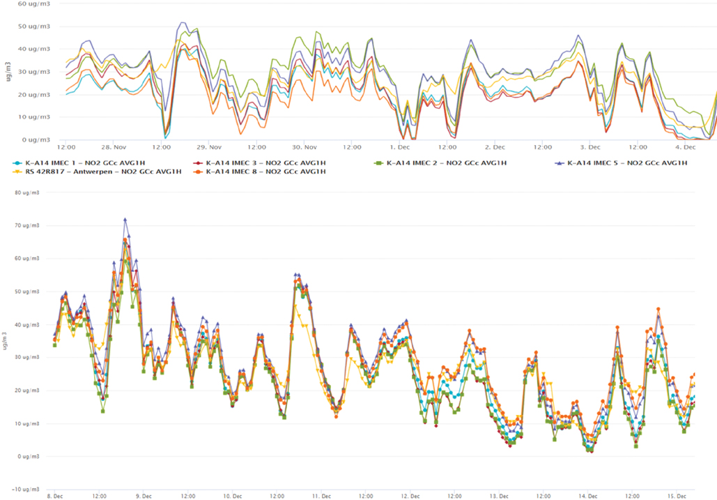
Figure 2. Hourly NO₂ co-location measurements of sensor batch 1 (IMEC1, IMEC2, IMEC3, IMEC5, and IMEC8) and regulatory data (42R817; yellow), when deployed before (27/11–5/12; upper) and after co-location calibration (8/12–17/12; lower).

3.1.2. Particulate matter

For PM, we observed a low intra-sensor variability (high precision), but varying comparability with the reference and with correlations in the order of PM₁ (R² = 0.44–0.85) > PM_2.5 (R² = 0.49–0.67) > PM₁₀ (R² = 0.39–0.72) and significant underestimations, as provided in Supplementary Appendix S5. Moreover, the sensor/REF ratio varied over time, with alternating under- and overestimations (Supplementary Appendix S5). This might be due to a change in particle composition (different source contribution) altering the refractive index and resulting mass concentrations derived by the sensors. Although the best calibration potential was obtained for PM₁ (best correlation), we tried to optimize for PM₁₀ and applied a single mass factor (PM₁₀) for all size fractions to prevent calibrated sensor readings from resulting in higher concentrations for smaller particle size fractions (PM₁ > PM_2.5 > PM₁₀). The resulting calibration performance (Supplementary Appendix S4) was low with expanded uncertainties (U_exp) ranging from sensitizing to inadequate (Supplementary Appendix S3). The average values of the performance statistics (R², MAE, RMSE, W_cm, and U_exp) of the 20 sensor systems (IMEC1–IMEC20) for each pollutant are listed in Table 2. A recent study on sensor evaluation also documented a low performance of the considered PM sensor (10). However, a different calibration procedure, e.g., a continuous network-based procedure as the one applied by Wesseling et al. (15, 26), might compensate better for a changing PM and background composition and meteorological impact on the resulting PM sensor performance, especially when targeting long-term (i.e., multi-season) monitoring initiatives with low-cost sensors.

TABLE 2

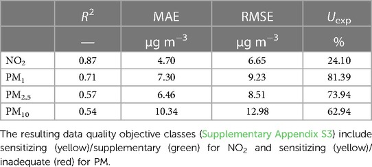
Table 2. Observed average sensor performance for all considered sensor units (IDs 1–20) after co-location calibration at a background AQMS (R817).

3.1.3. Impact of the sensor housing

In addition to the calibration performance, the impact from the mobile sensor housing was evaluated by comparing the Kunak sensors in both conditions: (i) mobile (enclosed housing with different openings and lamella to avoid turbulence over the sensors) and (ii) fixed shield (dedicated and more open housing for stationary conditions) (Figure 1). When the resulting concentrations were compared, the mobile housing resulted in lower particle concentrations (when stationary), while gas concentrations were similar between the fixed shield and mobile enclosure setup (Supplementary Appendix S6). We hypothesized that the design of the mobile housing, forcing the airflow over the internal lamella, favors particle interception through inertial impaction or electrostatic ionization, lowering the amount of measurable particles. This effect might be overruled at higher airflows, when the sensor is mobile or when the sensor housing is actively ventilated. Nevertheless, due to the lower sensor performance, observed impacts from the sensor housing, and the high prevalence (94%) of stationary operation conditions during mobile deployment (Table 3), we decided to focus our spatial analysis on NO₂, which achieved overall good sensor performance (R²= 0.87, MAE = 4.7), both in fixed shield and mobile enclosure conditions.

TABLE 3

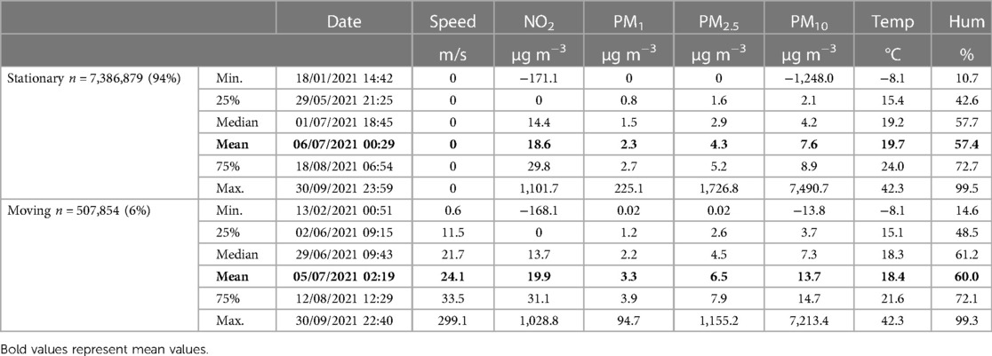
Table 3. Summary statistics of sensor data when stationary (speed = 0) and mobile (speed > 0).

3.1.4. Sensor performance throughout the project

During the 7-month mobile campaign, three sensor systems (IMEC18, IMEC19, and IMEC20) remained co-located at the R817 AQMS to evaluate their NO₂, PM_2.5, and PM₁₀ sensor performance over time. When the sensor performance at the beginning (February 19, 2021, to March 19, 2021; after co-location calibration) and end of the mobile campaign (September1, 2021, to October 1, 2021) was compared, a degrading sensor performance was observed over time (Figure 3). From the resulting regression plots (Figure 4), the association with reference NO₂ (R²) reduced from 0.87 to 0.73, 0.81 to 0.64, and 0.8 to 0.71 for IMEC18, IMEC19, and IMEC20, respectively. The MAEs increased from 5.82 to 8.67 µg/m³ (relative: 20%–35%), 12.75 to 14.37 µg/m³ (37%–51%), and 6.87 to 8.71 µg/m³ (22%–34%) for IMEC18, IMEC19, and IMEC20, respectively. The expanded uncertainty (U_exp) increases from 17%–61% to 53%–118%. The BSU reduced from 2.6 to 5.3 µg/m³, which is still acceptable for the network-based NO₂ sensor comparison since the observed urban spatial NO₂ gradients are often higher (Section 3.4).

FIGURE 3

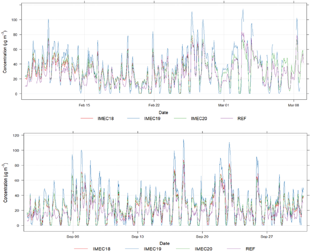
Figure 3. NO₂ time series of co-located sensor systems (IMEC18–IMEC20) and reference AQMS during the first (upper) and last (lower) month of the mobile monitoring campaign.

FIGURE 4

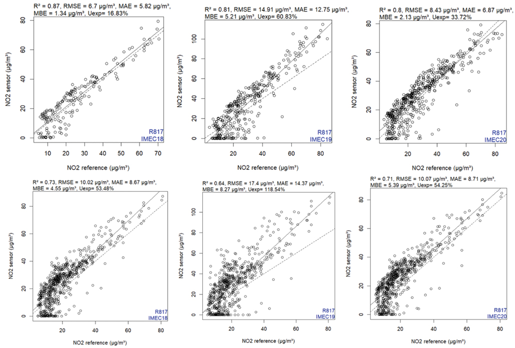
Figure 4. Scatterplots with associated performance statistics (R², RMSE MAE, MBE, and U_exp) of the collected sensor and reference data for IMEC18 (left), IMEC19 (middle), and IMEC20 (right) during the first (upper) and last (lower) month of the mobile monitoring campaign.

For PM_2.5 and PM₁₀, the regression plots and associated performance statistics, as provided in Supplementary Appendix S7 and S8, did not show clear degradation over time with similar or sometimes better performance observed at the end of the campaign. Nevertheless, this was hard to interpret due to the low performance of the initial sensors.

To investigate whether the degradation in NO₂ performance was related to sensor drift, we plotted the daily sensor/REF ratio over time (Figure 5). This graph revealed that the calibration event (19/2) was clearly reflected in better-aligned sensor/REF ratios. No consistent unidirectional deviation was observed over time. However, higher sensor/REF ratio amplitudes were observed between April and mid-August, possibly resulting from the seasonal variability in sensor confounders (Temp, RH, O₃). Lower calibration performance of similar NO₂ sensor systems during the (warmer and sunnier) summer season was previously observed from recurrent co-location campaigns (10), and this was confirmed when the mean hourly sensor/REF ratio was evaluated, in conjunction with temperature (°C) and RH (%), between the various seasons (Supplementary Appendix S9).

FIGURE 5

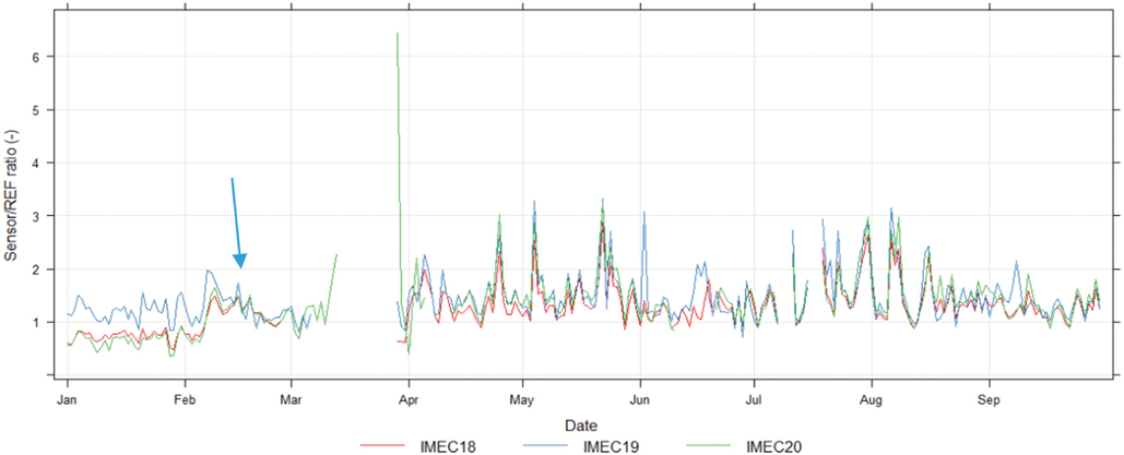
Figure 5. Time series of NO₂ sensor/REF ratio of AQMS co-located sensors IMEC18, IMEC19, and IMEC20.

3.2. Data exploration

The 17 mobile sensors were collected over 10 million data points between January and September 2021, and each data point consisted of measured concentrations of NO₂, PM₁, PM_2.5, and PM₁₀ (µg m⁻³), temperature (°C), humidity (%), GPS (Lat/Long), and driving speed (km h⁻¹). After bounding box selection for the city center of Antwerp and data cleaning were performed, 76% of the data (∼7.9 million data points) were retained. The monthly data coverage in a number of data points (#) and incremental area (%) and segment (#) coverage is provided in Supplementary Appendix S10 and visualized in Figure 6. Between January and September, 945 km of road was covered, yielding an average segment coverage of 1,050 measurements per street segment (median = 62). After 1 month of deployment, more than 50% of the street segments were covered by the sensor fleet. When all devices were on the road and configured at a 10-s monitoring resolution (May onward), a linear rise in segment coverage of ∼200 measurements per segment per month was observed. We, therefore, conclude that opportunistic data collection using service fleet vehicles (e.g., postal vans) is an efficient approach for rapidly covering a wide spatial area.

FIGURE 6

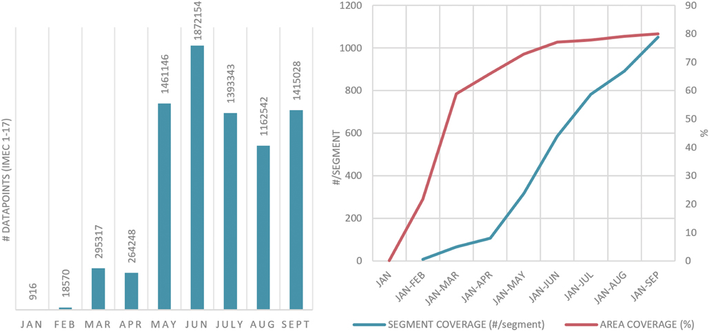
Figure 6. Left: monthly data collection by the 17 mobile sensor units (IMEC1–IMEC17) between January and September 2021. Right: resulting incremental area coverage (% street length covered) and segment coverage (#data points/segment).

The number of monthly data points reflected the consecutive batch calibrations at a lower monitoring resolution (5 min) between January and March (n = 916–53,681), remote configuration issues increasing the monitoring resolution to 10 s in April (n = 264,412–341,600), and successful high-resolution (10 s) monitoring for all devices from May to September (>1 million data points/month).

Similar data distributions were observed when the 17 sensors (Figure 7) were compared. Pollutant distributions were also similar when moving (speed >0) to stationary (speed = 0) conditions were compared. We found that 94% (n = 7,386,879) of the collected measurements were stationary (speed = 0), while sensors were only moving for 6% (n = 507,854) of the time, reflecting the frequent delivery stops of the vans on their service routes. When summary statistics between stationary and moving conditions were compared, slightly higher pollutant concentrations (NO₂, PM_x) and similar temperature and RH were obtained when mobile (Table 3). This might be caused by the observed impact of the enclosure on PM mass concentrations (Supplementary Appendix S6) and the contribution of evening and nighttime data (∼18–6 h), when all postal vans are parked at the postal depot which can be considered as an urban background location.

FIGURE 7

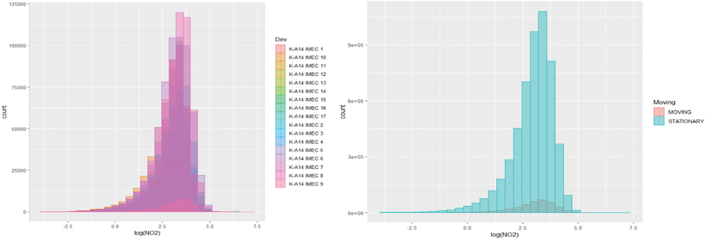
Figure 7. Log-transformed NO₂ data distributions for each mobile sensor unit (left) and during moving and stationary conditions (right).

3.3. Spatial aggregation

Spatial aggregation of the mobile measurements was required to derive spatial exposure maps for our study area. We decided to spatially aggregate the data to an openly available road segment map (wegenregister Antwerpen; https://portaal-stadantwerpen.opendata.arcgis.com/; accessed September 2022). In addition, we selected the road segments located in our study area (n = 6,447) and mapped the mobile measurements to the road segments by defining 10-m wide buffer areas for each road (line) segment in the QGIS software. Mobile measurements were subsequently clipped to these buffers, and pollutant and data coverage summary statistics were calculated for each month, progressive months (January–February, January–March, and so on) and for the entire dataset (January–September), as shown in Figure 8. Between January and September, 3,600 street segments (56%) were sampled, of which 3,369 street segments (52%) had at least two measurements and 2,729 street segments (42%) had at least 10 measurements. The highest data coverage was obtained at the postal depot (n = 1,809,269), followed by the long road segments that can be considered important traffic arteries of the city (e.g., Frankrijklei, Mechelsesteenweg, and Italiëlei). The street segment with the highest segment coverage (n = 16,350) and average street segment length (313 m) was the Quellinstraat.

FIGURE 8

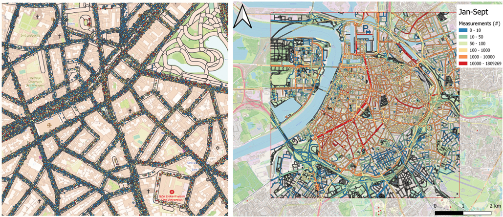
Figure 8. Street segment aggregation of mobile data points (left) and resulting street segment data coverage (#data points/segment) map of Antwerp (right). Dark gray-colored segments in the right panel did not contain any data points. The location of the postal depot is indicated by the parking icon.

3.4. Spatiotemporal pollutant distribution in Antwerp

From the collected mobile data points, monthly maps were created to evaluate the spatiotemporal pollutant variability and stability of the data coverage (#data points/segment) over time (Figure 9). An associated monthly summary statistics for each considered pollutant, temperature, and RH is provided in Table 4. From the resulting monthly point cloud maps, consecutive sensor batch deployments resulted in an increasing number of data points between January and April 2021, after which a fairly stable spatial coverage (May–September) was obtained over the entire city center (area within ring road), except for a southeastern district that was only poorly covered by the service fleet vehicles. Compared to PM, NO₂ exhibited a higher spatial variability over the city, with highest concentrations found along the ring road and major traffic axes (e.g., Plantin & Moretuslei, Leien). This was not surprising as NO₂ can be regarded as a typical traffic tracer. When the monthly maps (Figure 9) were compared, the spatial NO₂ variability was quite consistent throughout the mobile monitoring campaign. Spatial gradients (<10–50 µg/m³) greatly exceeded the observed BSU for NO₂ (2.6–5.3 µg/m³), which is important for network-based applications, because the observed spatial variability cannot be attributed to the measurement uncertainty between the sensors, but rather to local differences in pollution exposure. In addition to the expected busy traffic locations, higher NO₂ concentrations were also observed at unexpected locations within residential areas, highlighting local difficult traffic junctions or constrictions. While some of these hotspot locations were only sampled sporadically and, therefore, not representative, some had a proper recurrence and were consistently observed throughout the considered sampling months. These unexpected hotspot locations, discovered via this mobile monitoring approach, were noteworthy as they might prioritize future locations for targeted policy measures.

FIGURE 9

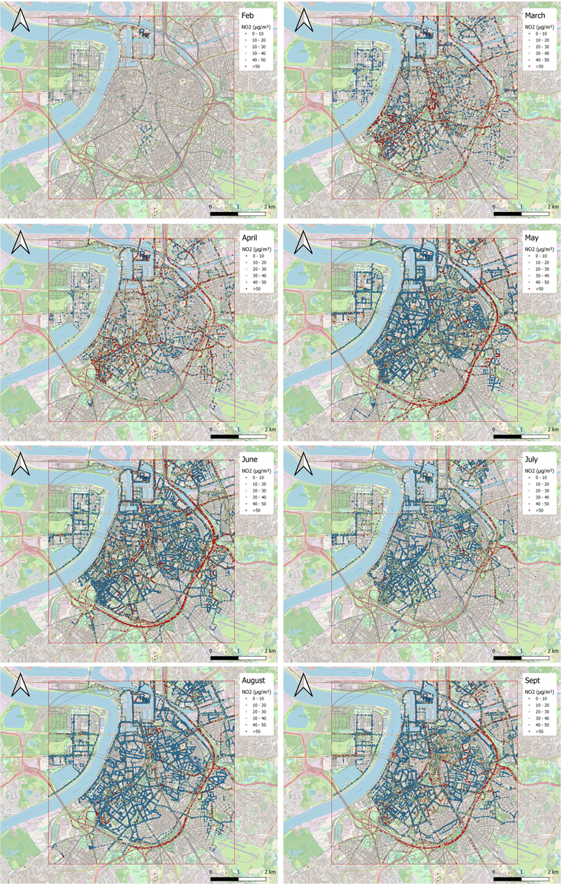
Figure 9. Maps of monthly collected mobile NO₂ measurements (µg m⁻³) in the city of Antwerp (BE) between February and September 2021.

TABLE 4

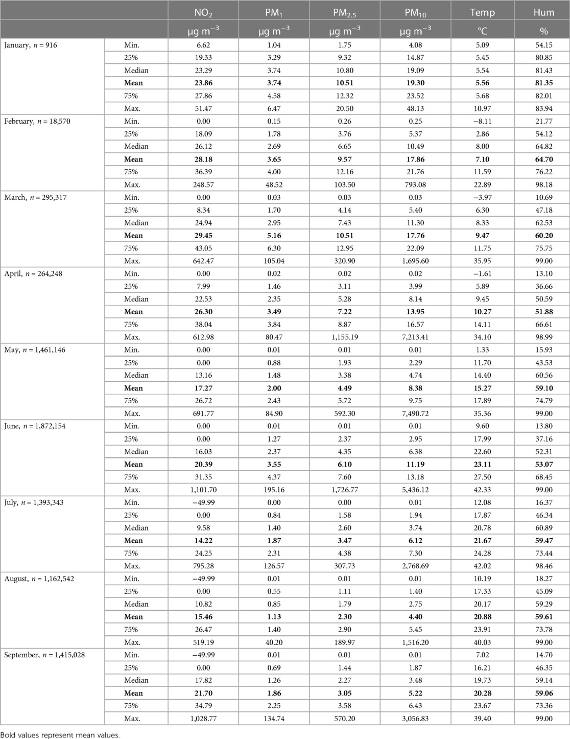
Table 4. Monthly data coverage (n) and summary statistics (min, 25%, median, mean, 75%, max) of the 17 mobile sensor systems for NO₂ (µg m⁻³), PM₁ (µg m⁻³), PM_2.5 (µg m⁻³), PM₁₀ (µg m⁻³), temperature (°C), and relative humidity (%).

When the temporal variability for NO₂ and PM at the hourly, daily, and monthly level (averages calculated based on the entire dataset) was evaluated, a distinct diurnality was observed for NO₂ with morning and evening rush hour peaks, slightly later evening peaks on Friday and Saturday, and overall lower pollutant concentrations throughout the weekend. This typical diurnality was consistently observed for all different sensor systems/vehicles (Supplementary Appendix S11) and was not surprising as NO₂ can be regarded as a typical tracer for road traffic (57–63). Seasonal variability was associated with lower NO₂ (<19.8 µg m⁻³) and PM (<14.5 µg m⁻³) concentrations during the summer months (May–August), while the highest average concentrations for NO₂ (28 µg m⁻³) and PM₁₀ (17.8 µg m⁻³) were observed in March.

Diurnality for PM is far less pronounced with low concentration increases (∼2 µg/m³) during morning hours and elevated concentrations on Sunday (when stationary at the postal depot). In terms of seasonality, higher concentrations are observed during the winter/spring period (January–April), when compared to the summer period (May–August). In September, concentrations start rising again for both NO₂ and PM (Figure 10).

FIGURE 10

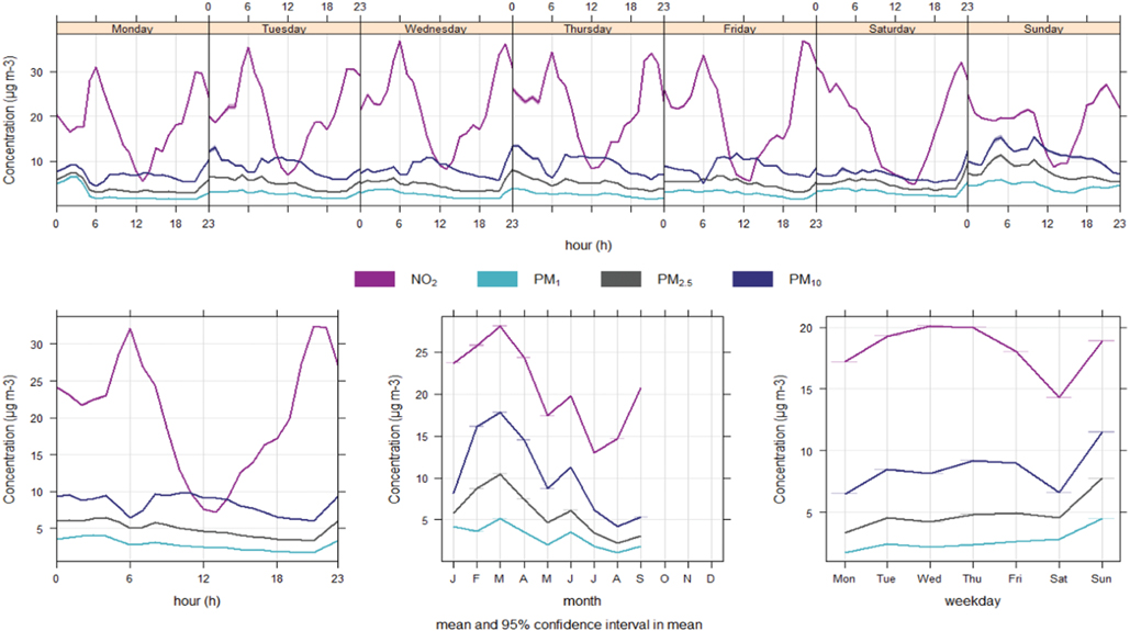
Figure 10. Hourly, daily, and monthly variability of the NO₂ (µg m⁻³), PM₁ (µg m⁻³), PM_2.5 (µg m⁻³), and PM₁₀ (µg m⁻³) measurements collected by the mobile sensor fleet (all sensors).

When comparing the temporal variability of the sensor fleet to the available stationary AQMS at different urban microenvironments (background, roadside, street canyon and ring road) in Antwerp, we found that the NO₂ dynamics (diurnality and seasonality) captured by the sensor fleet were also observed at the stationary AQMS network (Supplementary Appendix S12). The absolute hourly averaged concentration range of the sensor fleet (7–27 µg/m³) is slightly lower than the observed concentration range (15–45 µg/m³) of the regulatory stations (background <> ring road). Moreover, there was an earlier onset and decline of the morning rush hour peak in the sensor fleet NO₂ data, when compared to the AQMS. This observation cannot be explained by an environmental confounder on the sensor performance [e.g., temperature effect on sensor/REF ratio (Supplementary Appendix S9)], but it is believed to be caused by the fleet operation with an early start of the service rounds (∼5 h in Supplementary Appendix S1) and impact from remaining postal vans parked at the postal depot (background location). Nevertheless, the existing AQMS quite reflected the hourly observed NO₂ exposure range documented by the mobile measurements.

For PM_2.5, the sensor fleet followed the same trend (except between 5 and 7 h; humidity overcompensation?) but significantly underestimated the actual PM concentrations by ∼50%, as observed in the prior co-location campaign (Section 3.1.2). Moreover, the observed diurnality for PM is low (∼5 µg/m³), especially when compared to the observed sensor accuracy (error bars in Figure 11) in the prior co-location campaign indicating that the temporal PM variability cannot be properly assessed by the sensor network.

FIGURE 11

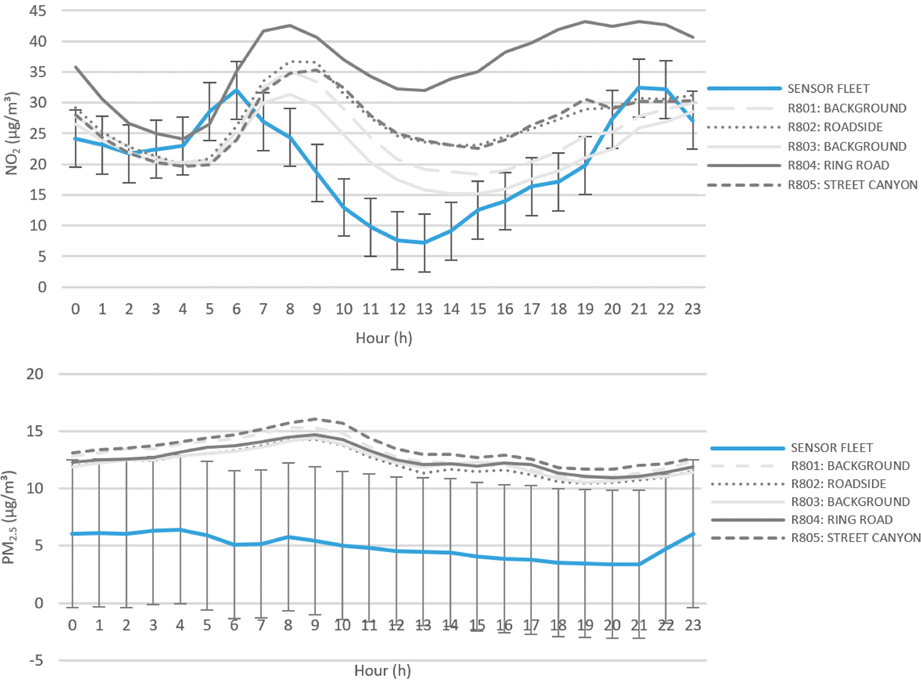
Figure 11. Fleet-averaged diurnal NO₂ (upper) and PM (lower) variability compared against fixed AQMS in different microenvironments (background, roadside, street canyon, and ring road) in Antwerp. The error bars represent the MAE, derived from the co-location calibration (Table 2).

3.5. Spatial exposure representativity

When all NO₂ measurements collected by our mobile sensor fleet (Figure 9) are combined, a map of the street segment averaged NO₂ concentrations can be derived visualizing the spatial variability in urban NO₂ exposure (Figure 12).

FIGURE 12

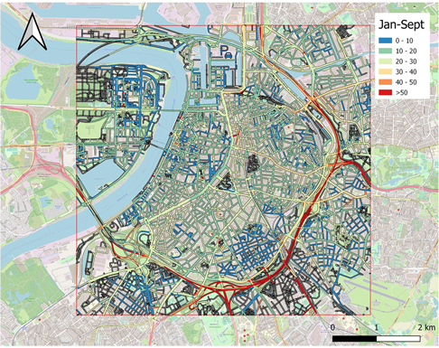
Figure 12. Street segment averaged NO₂ exposure map for Antwerp. The location of the postal depot is indicated by the parking icon.

To construct a representative map, we should consider the temporal (diurnal/monthly/seasonal) pollutant variability in our mobile sampling strategy. If a mobile sensor passes a street during early morning (<6 h) or around noon (∼12 h), lower concentrations of traffic-related pollutants will be measured than if the van passes the same street in rush hour traffic. Our sampling strategy is opportunistic, and therefore not controlled in terms of routing and sampling hours. The ways of coping with this temporal variability in the data analysis can be a background normalization (limited to an hourly resolution of the AQMS), modeling of the time variance in either land use regression (LUR) (64, 65) or machine learning models (35, 66), or considering enough repeated runs in the sampling strategy (67, 68).

In practice, a balance has to be found between (1) enough repeated measurements (passages) along each street segment to be representative of the monthly/long-term pollution exposure and (2) the effort/budget needed in terms of number of sensors, maintenance, and calibration. Previous studies applied subsampling strategies to derive the required number of passages to be representative (R²/error of the mean) for a certain street, route, and/or city (19, 69). We performed a similar exercise by extracting all mobile data points for the densely covered street segment Quellinstraat (n = 16,349). Because not all 10-s measurements can be regarded as independent passages, we first sorted the data according to timestamp and device, evaluated the timestep difference between consecutive measurements, and defined new passages for sequential timestep differences exceeding 15 min (to cope with longer stops/deliveries). This resulted in 879 unique passages (∼5% of original data).

To derive the required number of repeated measurements for them to be representative of the long-term average NO₂ exposure, we applied the methodology of Van Den Bossche et al. (67) on the Quellinstraat data. Because no reference data was available for the long-term average NO₂ concentration, we assumed that the average NO₂ based on the 879 passages (26.6 µg/m³) can be considered representative of the long-term average NO₂ concentration (gray line in the figure).

The passage-averaged NO₂ concentrations were randomly subsampled using sampling with replacement (passage means can be selected more than once) in R, with incrementing subsample size, from n = 1 to 879, and average NO₂ concentration calculated for each increasing subsample. This process was subsequently repeated 100 times (where each repeat is a random combination of passage means), and the resulting subsample averages were plotted against their subsample size (Figure 13). This graph revealed that the subsample means rapidly converge toward the long-term mean when the number of passages falls within the defined error bounds (red) after approximately ∼45 passages (Table 5).

FIGURE 13

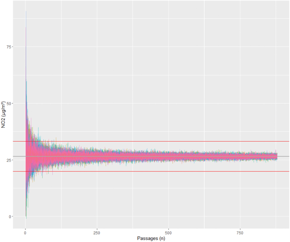
Figure 13. Subsampling analysis of the passage mean NO₂ concentrations (n = 879): average subsample concentrations are plotted against the incrementing subsample size from 1 to 879 (number of passages) and repeated 100 times (colored lines). The gray reference line represents the long-term mean calculated from the 879 passages (26.6 µg/m³), while both red lines represent the 25% bounds of the mean.

TABLE 5

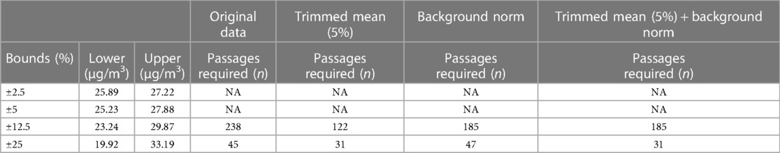
Table 5. Required number of passages (n) to have a 95% probability to be within ±2.5%, 5%, 12.5%, and 25% of the long-term average NO₂ concentration of the Quellinstraat, with associated lower and upper bounds (µg/m³) of the mean (26.6 µg/m³).

The number of required passages to have a 95% probability, to be within ±2.5%, 5%, 12.5%, and 25% of the long-term average NO₂ concentration (26.6 µg/m³), was subsequently derived from the 100 repeated subsamples (with n = 1–879), as summarized in Table 5. Based on the original passage means, 238 and 45 passages, respectively, are needed to have a 95% probability to be within ±12.5 and ±25% of the long-term mean of the Quellinstraat. Two post-processing approaches were tested to reduce these numbers, namely, the trimmed mean, where ±2.5% extremes were omitted from the passage means dataset, and an additive background normalization which was proposed by Dons et al. (70), where each passage mean ($\mathrm{N}{\mathrm{O}}_{2\mathrm{passage},i}$) was corrected for the exhibited hourly background concentration ($\mathrm{N}{\mathrm{O}}_{2\mathrm{background},i}$) and normalized to the long-term average background ($\mathrm{N}{\mathrm{O}}_{2\mathrm{background},\mathrm{long}\text{-}\mathrm{term}}$), as shown in Equation 3.

$\mathrm{N}{\mathrm{O}}_{2\mathrm{norm}}=\mathrm{N}{\mathrm{O}}_{2\mathrm{passage},i}-\mathrm{N}{\mathrm{O}}_{2\mathrm{background},i}+\mathrm{N}{\mathrm{O}}_{2\mathrm{background},\mathrm{long}\text{-}\mathrm{term}}(3)$

Both post-processing approaches result in a reduced number of required passages (Table 5), where the highest impact is observed for the trimmed mean, with 122 and 31 required passages to have a 95% probability to be within ±12.5% and ±25% of the long-term mean. Combining both procedures does not result in additional reductions.

When the Quellinstraat measurement/passage ratio (∼5.4%) was generalized for all other street segments, the required number of measurements would be 837 (16,349 measurements/879 passages × 45 required passages). After the selection of street segments with more than 837 measurements, 495 street segments remain, resulting in a representative long-term NO₂ exposure map of Antwerp (Figure 14).

FIGURE 14

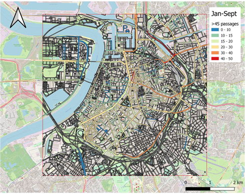
Figure 14. Representative long-term NO₂ exposure map, for all street segments (n = 495) containing more than 837 measurements (>45 passages). The location of the postal depot is indicated by the parking icon.

However, the required number of passages will depend on the characteristics of the street segments as they vary in terms of length, architecture (height/width ratio, openness), local source behavior, and resulting pollutant variability. Van Den Bossche et al. (67) found that the required number of passages for convergence varied widely when considering measured black carbon (BC) concentrations in different 50 m street segments along a cycling route, with 33–141 required passages to obtain convergence (95% probability and 25% deviation). After applying trimmed mean and background normalization, we found that these numbers were further reduced to 24–94 (10 and 90 percentiles of the 50-m segments). Through systematic subsampling of mobile car measurements in Oakland, Apte et al. (19) found that 10–20 drive days were sufficient to reproduce key spatial patterns of BC and NO with good precision and low bias. They achieved the mean R² for BC and NO approaching 0.7 after 10 days of driving and 0.9 after 20–25 days of driving.

Several studies looked into the long-term representativity of short-term measurement campaigns and the impact of monitoring strategy (locations, times, repeats, duration), indicating a variety of requirements depending on the pollutants considered, locations, time of sampling, sampling duration, and data-only vs. model approach. Messier et al. (24) compared 50 repeated measurements along a car route in Oakland to a LUR-Kriging model and found that data-only mapping outperformed the LUR-Kriging model in terms of cross-validation R² within four to eight repeated runs per road segment. In their recent study, Blanco et al. (71) investigated the impacts of various monitoring strategies in terms of number of sites (measurement locations), site visits (repeated measurements), time of sampling (during the day/week), and sampling time (duration) on the resulting long-term air pollution assessment for ultrafine particles, BC, NO₂, PM, and CO₂, based on a 278 sites × 26 visits dataset. They concluded that mobile monitoring campaigns wanting to assess long-term exposure should carefully consider their monitoring designs.

A sensitivity analysis on the required number of passages for convergence in our dataset will be the subject of a follow-up paper.

4. Conclusions

This study aimed to examine the validity of a mobile IoT sensor fleet for urban exposure assessments in Antwerp, a medium-sized and densely populated city in Belgium. The validity of the approach was evaluated holistically, from the design of the sensor network, proper validation and calibration procedure, mobile data processing, and analysis of spatiotemporal data coverage and representativity. We revealed that sensor calibration and validation are indispensable when applying low-cost air quality sensors in mobile settings. Indicative sensor performance was achieved after co-location calibration for NO₂, although PM exhibited unsatisfactory performance. A different PM sensor, mobile housing or calibration procedure (e.g., continuous, network-based calibration), might result in better PM results. We believe that continuous network-based calibration procedures should be the main focus of future research, especially when targeting long-term (i.e., multi-season) monitoring initiatives with low-cost sensors. In doing so, the availability of a reference instrument or regulatory monitoring network is indispensable.

Our mobile sensor fleet collected an extensive air quality dataset in Antwerp between February and September 2021, covering 945 km of road by a total of ∼7.9 million data points, yielding an average segment coverage of 1,050 measurements per street segment (median = 62). From the proposed area (%) and street segment (n) coverage, we concluded that opportunistic data collection using service fleet vehicles (e.g., postal vans) is an efficient approach in rapidly covering a wide spatial area and collecting many repeated runs (∼200 measurements/segment/month). The monthly maps showed recurring pollution gradients with hotspot locations both at the suspected (e.g., traffic arteries) and unexpected locations, with observed increments greatly exceeding the observed sensor uncertainty. The NO₂ variability documented by the sensor fleet fell within the range of the existing air quality monitoring network showing that the five AQMS well reflected the urban exposure variability in Antwerp. From the representativity analysis, we showed that ∼45 repeated passages of the postal vans (31 passages after pre-processing) were required to achieve the long-term average NO₂ exposure.

Our findings suggested that opportunistic data collection using sensors on service fleet vehicles is a valid approach for pollution exposure assessments, through proper validation and calibration strategy. Temporary deployment of mobile sensors was a valuable approach for cities with a less extensive air quality monitoring network or those who want a more fine-grained mapping.

Data availability statement

The datasets presented in this study can be found in online repositories. The names of the repository/repositories and accession number(s) can be found in the article and the Mendeley Data repository (55).

Ethics statement

Ethical review and approval was not required for this study in accordance with the national legislation and the institutional requirements.

Author contributions

JH contributed to the conceptualization, investigation, data curation, formal analysis, validation, data visualization, and writing. EI-U and MH contributed to the methodology, software, resources, and review of the manuscript. JP and MP assisted in the validation and review. VM contributed to the conceptualization, investigation, supervision, funding acquisition, and review and editing process. All authors contributed to the article and approved the submitted version.

Funding

This work was supported by the Flanders Innovation and Entrepreneurship (VLAIO) City of Things program and the European Union's Horizon 2020 Research and Innovation Program under the project “Research Infrastructures Services Reinforcing Air Quality Monitoring Capacities in European Urban & Industrial AreaS (RI-URBANS)” (grant number 101036245).

Acknowledgments

We acknowledge the city of Antwerp, the Belgian postal service (BPost), Kunak Technologies, and IMEC Belgium for their support in setting up the mobile sensor network.

Conflict of interest

EI-U and MH were employed by Kunak Technologies. The authors declare the involvement of Kunak Technologies in this study. Kunak provided support in setting up the mobile sensor network but was not involved in the study design, analysis, interpretation of data, the writing of this article or the decision to submit it for publication. The authors otherwise declare that the research was conducted in the absence of any commercial or financial relationships that could be construed as a potential conflict of interest.

Publisher's note

All claims expressed in this article are solely those of the authors and do not necessarily represent those of their affiliated organizations, or those of the publisher, the editors and the reviewers. Any product that may be evaluated in this article, or claim that may be made by its manufacturer, is not guaranteed or endorsed by the publisher.

Supplementary material

The Supplementary Material for this article can be found online at: https://www.frontiersin.org/articles/10.3389/fenvh.2023.1232867/full#supplementary-material

References

1. Castell N, Dauge FR, Schneider P, Vogt M, Lerner U, Fishbain B, et al. Can commercial low-cost sensor platforms contribute to air quality monitoring and exposure estimates? Environ Int. (2017) 99:293–302. doi: 10.1016/j.envint.2016.12.007

PubMed Abstract | CrossRef Full Text | Google Scholar

2. Karagulian F, Barbiere M, Kotsev A, Spinelle L, Gerboles M, Lagler F, et al. Review of the performance of low-cost sensors for air quality monitoring. Atmosphere. (2019) 10:506. doi: 10.3390/atmos10090506

CrossRef Full Text | Google Scholar

3. Badura M, Batog P, Drzeniecka-Osiadacz A, Modzel P. Evaluation of low-cost sensors for ambient PM_2.5 monitoring. J Sens. (2018) 2018:1–16. doi: 10.1155/2018/5096540

CrossRef Full Text | Google Scholar

4. Desouza PN. Key concerns and drivers of low-cost air quality sensor use. Sustainability. (2022) 14:584. doi: 10.3390/su14010584

CrossRef Full Text | Google Scholar

5. Jayaratne R, Liu X, Thai P, Dunbabin M, Morawska L. The influence of humidity on the performance of low-cost air particle mass sensors and the effect of atmospheric fog. Atmos Meas Tech Discuss. (2018) 11(8):4883–90. doi: 10.5194/amt-11-4883-2018

CrossRef Full Text | Google Scholar

6. Vercauteren J. Performance evaluation of six low-cost particulate matter sensors in the field. Vaquums (2021). Available at: https://vaquums.eu/sensor-db/tests/life-vaquums_pmfieldtest.pdf/view

7. Wei P, Ning Z, Ye S, Sun L, Yang F, Wong KC, et al. Impact analysis of temperature and humidity conditions on electrochemical sensor response in ambient air quality monitoring. Sensors (Basel). (2018) 18:59. doi: 10.3390/s18020059

PubMed Abstract | CrossRef Full Text | Google Scholar

8. Clements AL, Griswold WG, Abhijit RS, Johnston JE, Herting MM, Thorson J, et al. Low-cost air quality monitoring tools: from research to practice (a workshop summary). Sensors (Basel). (2017) 17(11):2478. doi: 10.3390/s17112478

PubMed Abstract | CrossRef Full Text | Google Scholar

9. Hofman J, Nikolaou M, Shantharam SP, Stroobants C, Weijs S, La Manna VP. Distant calibration of low-cost PM and NO₂ sensors; evidence from multiple sensor testbeds. Atmos Pollut Res. (2022b) 13:101246. doi: 10.1016/j.apr.2021.101246

CrossRef Full Text | Google Scholar

10. Hofman J, Peters J, Stroobants C, Elst E, Baeyens B, Laer JV, et al. Air quality sensor networks for evidence-based policy making: best practices for actionable insights. Atmosphere. (2022) 13:944. doi: 10.3390/atmos13060944

CrossRef Full Text | Google Scholar

11. Munir S, Mayfield M, Coca D, Jubb SA, Osammor O. Analysing the performance of low-cost air quality sensors, their drivers, relative benefits and calibration in cities—a case study in Sheffield. Environ Monit Assess. (2019) 191:94. doi: 10.1007/s10661-019-7231-8

PubMed Abstract | CrossRef Full Text | Google Scholar

12. Rai AC, Kumar P, Pilla F, Skouloudis AN, Di Sabatino S, Ratti C, et al. End-user perspective of low-cost sensors for outdoor air pollution monitoring. Sci Total Environ. (2017) 607–8:691–705. doi: 10.1016/j.scitotenv.2017.06.266

PubMed Abstract | CrossRef Full Text | Google Scholar

13. Spinelle L, Aleixandre M, Gerboles M. Protocol of evaluation and calibration of low-cost gas sensors for the monitoring of air pollution. Joint Research Centre (JRC) (2013). Available at: https://publications.jrc.ec.europa.eu/repository/handle/JRC83791

14. Van Zoest V, Osei FB, Stein A, Hoek G. Calibration of low-cost NO₂ sensors in an urban air quality network. Atmos Environ. (2019) 210:66–75. doi: 10.1016/j.atmosenv.2019.04.048

CrossRef Full Text | Google Scholar

15. Wesseling J, de Ruiter H, Blokhuis C, Drukker D, Weijers E, Volten H, et al. Development and implementation of a platform for public information on air quality, sensor measurements, and citizen science. Atmosphere. (2019) 10:445. doi: 10.3390/atmos10080445

CrossRef Full Text | Google Scholar

16. Cui H, Zhang L, Li W, Yuan Z, Wu M, Wang C, et al. A new calibration system for low-cost sensor network in air pollution monitoring. Atmos Pollut Res. (2021) 12(5):101049. doi: 10.1016/j.apr.2021.03.012

CrossRef Full Text | Google Scholar

17. De Vito S, Di Francia G, Esposito E, Ferlito S, Formisano F, Massera E. Adaptive machine learning strategies for network calibration of IoT smart air quality monitoring devices. Pattern Recognit Lett. (2020) 136:264–71. doi: 10.1016/j.patrec.2020.04.032

CrossRef Full Text | Google Scholar

18. Drajic DD, Gligoric NR. Reliable low-cost air quality monitoring using off-the-shelf sensors and statistical calibration. Elektronika ir Elektrotechnika. (2020) 26:32–41. doi: 10.5755/j01.eie.26.2.25734

CrossRef Full Text | Google Scholar

19. Apte JS, Messier KP, Gani S, Brauer M, Kirchstetter TW, Lunden MM, et al. High-resolution air pollution mapping with Google Street View cars: exploiting big data. Environ Sci Technol. (2017) 51:6999–7008. doi: 10.1021/acs.est.7b00891

PubMed Abstract | CrossRef Full Text | Google Scholar

20. Desouza P, Anjomshoaa A, Duarte F, Kahn R, Kumar P, Ratti C. Air quality monitoring using mobile low-cost sensors mounted on trash-trucks: methods development and lessons learned. Sustain Cities Soc. (2020) 60:102239. doi: 10.1016/j.scs.2020.102239

CrossRef Full Text | Google Scholar

21. Elen B, Peters J, Poppel MV, Bleux N, Theunis J, Reggente M, et al. The Aeroflex: a bicycle for mobile air quality measurements. Sensors (Basel). (2013) 13:221–40. doi: 10.3390/s130100221

CrossRef Full Text | Google Scholar

22. Hasenfratz D, Saukh O, Walser C, Hueglin C, Fierz M, Arn T, et al. Deriving high-resolution urban air pollution maps using mobile sensor nodes. Pervasive Mob Comput. (2015) 16:268–85. doi: 10.1016/j.pmcj.2014.11.008

CrossRef Full Text | Google Scholar

23. Kaivonen S, Ngai E. Real-time air pollution monitoring with sensors on city bus. Digit Commun Netw. (2019) 6(1):23–30. doi: 10.1016/j.dcan.2019.03.003

CrossRef Full Text | Google Scholar

24. Messier KP, Chambliss SE, Gani S, Alvarez R, Brauer M, Choi JJ, et al. Mapping air pollution with Google Street View cars: efficient approaches with mobile monitoring and land use regression. Environ Sci Technol. (2018) 52:12563–72. doi: 10.1021/acs.est.8b03395

PubMed Abstract | CrossRef Full Text | Google Scholar

25. Schulte N, Li X, Ghosh JK, Fine PM, Epstein SA. Responsive high-resolution air quality index mapping using model, regulatory monitor, and sensor data in real-time. Environ Res Lett. (2020) 15:1040a7. doi: 10.1088/1748-9326/abb62b

CrossRef Full Text | Google Scholar

26. Wesseling J, Hendricx W, De Ruiter H, Van Ratingen S, Drukker D, Huitema M, et al. Assessment of PM_2.5 exposure during cycle trips in the Netherlands using low-cost sensors. Int J Environ Res Public Health. (2021) 18(11):6007. doi: 10.3390/ijerph18116007

PubMed Abstract | CrossRef Full Text | Google Scholar

27. Mueller MD, Hasenfratz D, Saukh O, Fierz M, Hueglin C. Statistical modelling of particle number concentration in Zurich at high spatio-temporal resolution utilizing data from a mobile sensor network. Atmos Environ. (2016) 126:171–81. doi: 10.1016/j.atmosenv.2015.11.033

CrossRef Full Text | Google Scholar

28. Chen Y, Gu P, Schulte N, Zhou X, Mara S, Croes BE, et al. A new mobile monitoring approach to characterize community-scale air pollution patterns and identify local high pollution zones. Atmos Environ. (2022) 272:118936. doi: 10.1016/j.atmosenv.2022.118936

CrossRef Full Text | Google Scholar

29. Franco JF, Segura JF, Mura I. Air pollution alongside bike-paths in Bogotá-Colombia. Front Environ Sci. (2016) 4:77. doi: 10.3389/fenvs.2016.00077

CrossRef Full Text | Google Scholar

30. Hofman J, Samson R, Joosen S, Blust R, Lenaerts S. Cyclist exposure to black carbon, ultrafine particles and heavy metals: an experimental study along two commuting routes near Antwerp, Belgium. Environ Res. (2018) 164:530–8. doi: 10.1016/j.envres.2018.03.004

PubMed Abstract | CrossRef Full Text | Google Scholar

31. Genikomsakis KN, Galatoulas N-F, Dallas PI, Candanedo Ibarra LM, Margaritis D, Ioakimidis CS. Development and on-field testing of low-cost portable system for monitoring PM_2.5 concentrations. Sensors (Basel). (2018) 18(4):1056. doi: 10.3390/s18041056

PubMed Abstract | CrossRef Full Text | Google Scholar

32. Peters J, Van Den Bossche J, Reggente M, Van Poppel M, De Baets B, Theunis J. Cyclist exposure to UFP and BC on urban routes in Antwerp, Belgium. Atmos Environ. (2014) 92:31–43. doi: 10.1016/j.atmosenv.2014.03.039

CrossRef Full Text | Google Scholar

33. Qiu Z, Wang W, Zheng J, Lv H. Exposure assessment of cyclists to UFP and PM on urban routes in Xi’an, China. Environ Pollut. (2019) 250:241–50. doi: 10.1016/j.envpol.2019.03.129

PubMed Abstract | CrossRef Full Text | Google Scholar

34. Van Den Bossche J, Theunis J, Elen B, Peters J, Botteldooren D, De Baets B. Opportunistic mobile air pollution monitoring: a case study with city wardens in Antwerp. Atmos Environ. (2016) 141:408–21. doi: 10.1016/j.atmosenv.2016.06.063

CrossRef Full Text | Google Scholar

35. Hofman J, Do TH, Qin X, Bonet ER, Philips W, Deligiannis N, et al. Spatiotemporal air quality inference of low-cost sensor data: evidence from multiple sensor testbeds. Environ Model Softw. (2022) 149:105306. doi: 10.1016/j.envsoft.2022.105306

CrossRef Full Text | Google Scholar

36. Yuan Z, Kerckhoffs J, Hoek G, Vermeulen R. A knowledge transfer approach to map long-term concentrations of hyperlocal air pollution from short-term mobile measurements. Environ Sci Technol. (2022) 56:13820–8. doi: 10.1021/acs.est.2c05036

PubMed Abstract | CrossRef Full Text | Google Scholar

37. Jacobs L, Nawrot TS, De Geus B, Meeusen R, Degraeuwe B, Bernard A, et al. Subclinical responses in healthy cyclists briefly exposed to traffic-related air pollution: an intervention study. Environ Health. (2010) 9:64. doi: 10.1186/1476-069X-9-64

PubMed Abstract | CrossRef Full Text | Google Scholar

38. De Craemer S, Vercauteren J, Fierens F, Lefebvre W, Meysman F. Using large-scale NO₂ data from citizen science for air quality compliance and policy support. Environ Sci Technol. (2020) 54(18):11070–8. doi: 10.1021/acs.est.0c02436

PubMed Abstract | CrossRef Full Text | Google Scholar

39. VMM. Intra-urban variability of ultrafine particles in Antwerp (February and October 2013), D/2014/6871/065. (2014). Available at: https://publicaties.vlaanderen.be/view-file/15471

40. Hofman J, Castanheiro A, Nuyts G, Joosen S, Spassov S, Blust R, et al. Impact of urban street canyon architecture on local atmospheric pollutant levels and magneto-chemical PM₁₀ composition: an experimental study in Antwerp, Belgium. Sci Total Environ. (2019) 712:135534. doi: 10.1016/j.scitotenv.2019.135534

PubMed Abstract | CrossRef Full Text | Google Scholar

41. Hofman J, Staelens J, Cordell R, Stroobants C, Zikova N, Hama SML, et al. Ultrafine particles in four European urban environments: results from a new continuous long-term monitoring network. Atmos Environ. (2016) 136:68–81. doi: 10.1016/j.atmosenv.2016.04.010

CrossRef Full Text | Google Scholar

42. Mishra VK, Kumar P, Van Poppel M, Bleux N, Frijns E, Reggente M, et al. Wintertime spatio-temporal variation of ultrafine particles in a Belgian city. Sci Total Environ. (2012) 431:307–13. doi: 10.1016/j.scitotenv.2012.05.054

PubMed Abstract | CrossRef Full Text | Google Scholar

43. Degraeuwe B, Thunis P, Clappier A, Weiss M, Lefebvre W, Janssen S, et al. Impact of passenger car NOx emissions and NO₂ fractions on urban NO₂ pollution—scenario analysis for the city of Antwerp, Belgium. Atmos Environ. (2015) 126:218–24. doi: 10.1016/j.atmosenv.2015.11.042

CrossRef Full Text | Google Scholar

44. Hofman J, Bartholomeus H, Janssen S, Calders K, Wuyts K, Van Wittenberghe S, et al. Influence of tree crown characteristics on the local PM₁₀ distribution inside an urban street canyon in Antwerp (Belgium): a model and experimental approach. Urban For Urban Green. (2016) 20:265–76. doi: 10.1016/j.ufug.2016.09.013

CrossRef Full Text | Google Scholar

45. Hofman J, Lefebvre W, Janssen S, Nackaerts R, Nuyts S, Mattheyses L, et al. Increasing the spatial resolution of air quality assessments in urban areas: a comparison of biomagnetic monitoring and urban scale modelling. Atmos Environ. (2014) 92:130–40. doi: 10.1016/j.atmosenv.2014.04.013

CrossRef Full Text | Google Scholar

46. Lefebvre W, Van Poppel M, Maiheu B, Janssen S, Dons E. Evaluation of the RIO-IFDM-street canyon model chain. Atmos Environ. (2013) 77:325–37. doi: 10.1016/j.atmosenv.2013.05.026

CrossRef Full Text | Google Scholar

47. Nikolova I, Janssen S, Vos P, Vrancken K, Mishra V, Berghmans P. Dispersion modelling of traffic induced ultrafine particles in a street canyon in Antwerp, Belgium and comparison with observations. Sci Total Environ. (2011) 412–3:336–43. doi: 10.1016/j.scitotenv.2011.09.081

CrossRef Full Text | Google Scholar

48. Van BrusseleN D, Arrazola De Oñate W, Maiheu B, Vranckx S, Lefebvre W, Janssen S, et al. Health impact assessment of a predicted air quality change by moving traffic from an urban ring road into a tunnel. The case of Antwerp, Belgium. PLoS One. (2016) 11:e0154052. doi: 10.1371/journal.pone.0154052

PubMed Abstract | CrossRef Full Text | Google Scholar

49. Crilley LR, Singh A, Kramer LJ, Shaw MD, Alam MS, Apte JS, et al. Effect of aerosol composition on the performance of low-cost optical particle counter correction factors. Atmos Meas Tech. (2020) 13:1181–93. doi: 10.5194/amt-13-1181-2020

CrossRef Full Text | Google Scholar

50. Mijling B, Jiang Q, De Jonge D, Bocconi S. Field calibration of electrochemical NO₂ sensors in a citizen science context. Atmos Meas Tech. (2018) 11:1297–312. doi: 10.5194/amt-11-1297-2018

CrossRef Full Text | Google Scholar

51. Vikram S, Collier-Oxandale A, Ostertag MH, Menarini M, Chermak C, Dasgupta S, et al. Evaluating and improving the reliability of gas-phase sensor system calibrations across new locations for ambient measurements and personal exposure monitoring. Atmos Meas Tech. (2022) 12:4211–39. doi: 10.5194/amt-12-4211-2019

CrossRef Full Text | Google Scholar

52. Polidori A. AQ-SPEC field setup and testing evaluation protocol. AQ-SPEC (2017). Available at: http://www.aqmd.gov/docs/default-source/aq-spec/protocols/sensors-field-testing-protocol.pdf?sfvrsn=0

53. Weijers E, Vercauteren J, Van Dinther D. Performance evaluation of low-cost air quality sensors in the laboratory and in the field. VAQUUMS (2021). Available at: https://vaquums.eu/sensor-db/tests/protocols/life-vaquums_testprotocol_final.pdf/view

54. Yatkin S, Gerboles M, Borowiak A, Davila S, Spinelle L, Bartonova A, et al. Modified target diagram to check compliance of low-cost sensors with the data quality objectives of the European air quality directive. Atmos Environ. (2022) 273:118967. doi: 10.1016/j.atmosenv.2022.118967

CrossRef Full Text | Google Scholar

55. Hofman J, Panzica La Manna V, Ibarrola-Ulzurrun E, Escribano M. Mobile PM and NO₂ data collected by mobile sensors on postal vans in Antwerp, Belgium. Mendeley Dat, V1. (2023). doi: 10.17632/89vgprbzv3.1

56. Carslaw DC, Ropkins K. Openair: open-source tools for the analysis of air pollution data. R package version 1.1-5 ed. London: Natural Environment Research Council (2015).

57. De Craemer S, Vercauteren J, Fierens F, Lefebvre W, Meysman FJR. Using large-scale NO₂ data from citizen science for air-quality compliance and policy support. Environ Sci Technol. (2020) 54:11070–8. doi: 10.1021/acs.est.0c02436

PubMed Abstract | CrossRef Full Text | Google Scholar

58. Domínguez-López D, Adame JA, Hernández-Ceballos MA, Vaca F, De La Morena BA, Bolívar JP. Spatial and temporal variation of surface ozone, NO and NO₂ at urban, suburban, rural and industrial sites in the southwest of the Iberian Peninsula. Environ Monit Assess. (2014) 186:5337–51. doi: 10.1007/s10661-014-3783-9

CrossRef Full Text | Google Scholar

59. Munir S, Mayfield M, Coca D. Understanding spatial variability of NO₂ in urban areas using spatial modelling and data fusion approaches. Atmosphere. (2021) 12:179. doi: 10.3390/atmos12020179

CrossRef Full Text | Google Scholar

60. Hewitt CN. Spatial variations in nitrogen dioxide concentrations in an urban area. Atmos Environ Part B Urban Atmos. (1991) 25:429–34. doi: 10.1016/0957-1272(91)90014-6

CrossRef Full Text | Google Scholar

61. Niepsch D, Clarke LJ, Tzoulas K, Cavan G. Spatiotemporal variability of nitrogen dioxide (NO₂) pollution in Manchester (UK) city centre (2017–2018) using a fine spatial scale single-NOx diffusion tube network. Environ Geochem Health. (2022) 44:3907–27. doi: 10.1007/s10653-021-01149-w

PubMed Abstract | CrossRef Full Text | Google Scholar

62. Pirjola L, Lähde T, Niemi JV, Kousa A, Rönkkö T, Karjalainen P, et al. Spatial and temporal characterization of traffic emissions in urban microenvironments with a mobile laboratory. Atmos Environ. (2012) 63:156–67. doi: 10.1016/j.atmosenv.2012.09.022

CrossRef Full Text | Google Scholar

63. Solomon PA, Vallano D, Lunden M, Lafranchi B, Blanchard CL, Shaw SL. Mobile-platform measurement of air pollutant concentrations in California: performance assessment, statistical methods for evaluating spatial variations, and spatial representativeness. Atmos Meas Tech. (2020) 13:3277–301. doi: 10.5194/amt-13-3277-2020

CrossRef Full Text | Google Scholar

64. Kerckhoffs J, Khan J, Hoek G, Yuan Z, Ellermann T, Hertel O, et al. Mixed-effects modeling framework for Amsterdam and Copenhagen for outdoor NO₂ concentrations using measurements sampled with Google Street View cars. Environ Sci Technol. (2022) 56(11):7174–84. doi: 10.1021/acs.est.1c05806

PubMed Abstract | CrossRef Full Text | Google Scholar

65. Van Den Bossche J, De Baets B, Botteldooren D, Theunis J. A spatio-temporal land use regression model to assess street-level exposure to black carbon. Environ Model Softw. (2020) 133:104837. doi: 10.1016/j.envsoft.2020.104837

CrossRef Full Text | Google Scholar

66. Do TH, Tsiligianni E, Qin X, Hofman J, La Manna VP, Philips W, et al. Graph-deep-learning-based inference of fine-grained air quality from mobile IoT sensors. IEEE Internet Things J. (2020) 7(9):8943–55. doi: 10.1109/JIOT.2020.2999446

CrossRef Full Text | Google Scholar

67. Van Den Bossche J, Peters J, Verwaeren J, Botteldooren D, Theunis J, De Baets B. Mobile monitoring for mapping spatial variation in urban air quality: development and validation of a methodology based on an extensive dataset. Atmos Environ. (2015) 105:148–61. doi: 10.1016/j.atmosenv.2015.01.017

CrossRef Full Text | Google Scholar

68. Van Poppel M, Peters J, Bleux N. Methodology for setup and data processing of mobile air quality measurements to assess the spatial variability of concentrations in urban environments. Environ Pollut. (2013) 183:224–33. doi: 10.1016/j.envpol.2013.02.020

PubMed Abstract | CrossRef Full Text | Google Scholar

69. Van Den Bossche J. Towards high spatial resolution air quality mapping: a methodology to assess street-level exposure based on mobile monitoring. [doctoral thesis]. Ghent University (2016).

70. Vandeninden B, Vanpoucke C, Peeters O, Hofman J, Stroobants C, De Craemer S, et al. Uncovering spatio-temporal air pollution exposure patterns during commutes to create an open-data endpoint for routing purposes. In: Krevs M, editor. Hidden geographies. Key Challenges in Geography. Cham: Springer International Publishing (2021). doi: 10.1007/978-3-030-74590-5

71. Blanco MN, Bi J, Austin E, Larson TV, Marshall JD, Sheppard L. Impact of mobile monitoring network design on air pollution exposure assessment models. Environ Sci Technol. (2023) 57:440–50. doi: 10.1021/acs.est.2c05338

PubMed Abstract | CrossRef Full Text | Google Scholar